
Stochastic Drift Counteraction Optimal Control of a Fuel Cell-Powered Small Unmanned Aerial Vehicle


1
Department of Aerospace Engineering, University of Michigan, Ann Arbor, MI 48109, USA
2
Department of Naval Architecture and Marine Engineering, University of Michigan, Ann Arbor, MI 48109, USA
*
Author to whom correspondence should be addressed.
Energies 2021, 14(5), 1304; https://doi.org/10.3390/en14051304
Submission received: 31 January 2021
/
Revised: 20 February 2021
/
Accepted: 22 February 2021
/
Published: 27 February 2021
(This article belongs to the Special Issue Advanced Control and Estimation Concepts, and New Hardware Topologies for Future Mobility)
Abstract
:This paper investigates optimal power management of a fuel cell hybrid small unmanned aerial vehicle (sUAV) from the perspective of endurance (time of flight) maximization in a stochastic environment. Stochastic drift counteraction optimal control is exploited to obtain an optimal policy for power management that coordinates the operation of the fuel cell and battery to maximize the expected flight time while accounting for the limits on the rate of change of fuel cell power output and the orientation dependence of fuel cell efficiency. The proposed power management strategy accounts for known statistics in transitions of propeller power and climb angle during the mission, but does not require the exact preview of their time histories. The optimal control policy is generated offline using value iterations implemented in Cython, demonstrating an order of magnitude speedup as compared to MATLAB. It is also shown that the value iterations can be further sped up using a discount factor, but at the cost of decreased performance. Simulation results for a kg sUAV are reported that illustrate the optimal coordination between the fuel cell and the battery during aircraft maneuvers, including a turnpike in the battery state of charge () trajectory. As the fuel cell is not able to support fast changes in power output, the optimal policy is shown to charge the battery to the turnpike value if starting from a low initial value. If starting from a high value, the battery energy is used till a turnpike value of the is reached with further discharge delayed to later in the flight. For the specific scenarios and simulated sUAV parameters considered, the results indicate the capability of up to h of flight time.
1. Introduction
With the growing market for unmanned aerial vehicles (UAVs), a wide range of industries and organizations, including military, government, industrial, and recreational users, deploy this technology across the globe [1,2,3]. Among different types of UAVs, small unmanned aerial vehicles (sUAVs) [4] are attractive for military, aerial photography, and environmental monitoring applications due to their small size and flexible operation [5]. Considering the (i) hardware and weight constraints, (ii) limited onboard energy storage, and (iii) performance requirements for sUAVs, improving their endurance (maximizing their flight time) is of great importance for extending the duration of their missions, which could involve surveillance, search and rescue, disaster relief, traffic control, and precision agriculture, thereby motivating the development of novel propulsion systems and the implementation of optimal control policies for power and energy management. Among different propulsion systems for such sUAVs, a hybrid propulsion system consisting of a polymer electrolyte membrane fuel cell (PEMFC) and a battery has been proposed for long duration missions, e.g., in [6,7,8,9]. Other propulsion systems may incorporate energy harvesters, such as in [10]. In this paper we focus on novel approaches to the energy management of sUAVs through optimal coordination between the PEMFC and battery for the previously proposed fuel cell hybrid propulsion system.
Rule-based (e.g., thermostat-like on-off control [11]), dynamic programming-based [12], and model predictive control (MPC) [13] methods have been considered for the energy management of hybrid aircraft. As in automotive energy management applications [14], the use of simple rule-based strategies may not provide optimal performance, while the conventional formulations of MPC and dynamic programming do not directly address the flight time maximization objective. Furthermore, deterministic variants of MPC and dynamic programming may require an accurate preview of the propeller power and climb angle over a long horizon and are computationally demanding if optimization has to be performed online. Similarly, the Pontryagin maximum principle (PMP)-based guidance solutions [15] need accurate characterization of the flight environment.
In this paper, we consider a different approach to the problem of endurance maximization for a hybrid UAV with a polymer electrolyte membrane fuel cell (PEMFC) based on an application of stochastic drift counteraction optimal control (SDCOC) [16], which directly addresses the problem of maximizing the time to constraint violation in a stochastic environment. In our case, the objective is to maintain the vehicle flying for a maximum amount of time by coordinating the fuel cell and the battery to provide the requested propeller power subject to the limited amount of fuel and battery state of charge () onboard the vehicle. The transitions in aircraft climb angle and propeller power are modeled stochastically by a Markov chain with the transition probabilities determined from historical data representing typical missions of an sUAV. Then, a control policy that minimizes a cost functional reflective of expected time-to-violate constraints is determined offline through value iterations; this control policy is then deployed onboard for the online coordination of the fuel cell and the battery in the sUAV.
In a preliminary conference paper [17] by the second author of this paper, the application of SDCOC for power management of a hybrid sUAV with a direct methanol fuel cell (DMFC) was considered. While the DMFC is often considered as a suitable power source for ground vehicles [18] and has certain advantages, PEMFCs are more appealing for air mobility applications [6,7] due to their relatively lower operating temperature, allowing for a quick start-up [19], higher efficiency (up to 60% [18,20]) and power density, and higher safety due to the use of the solid electrolyte [18].
Different from [17], in this paper, we consider the application of SDCOC to the power management of a hybrid sUAV with a PEMFC rather than a DMFC. To accommodate a different fuel cell and an sUAV, the fuel cell model is changed and improvements are made to the models used to compute the propeller power and thrust, as well as the evolution of the .
More importantly, the lack of the ability of the PEMFC to rapidly change its power output imposes a stringent operating constraint (rate limit on PEMFC power output), which was not treated in [17], but is treated in this paper. This rate limit increases the complexity of the problem as an extra state needs to be introduced in the model and handled in SDCOC, and it also changes the optimal policies and the optimal response of the system. For instance, as the fuel cell is not able to support fast changes in power output, the optimal policy is shown to charge the battery to a turnpike value if starting from a low initial state of charge value. If starting from a high , the battery energy is used till a turnpike value of the state of charge is reached with further discharge delayed to a later phase of the flight. In either case, the high frequency chattering of fuel cell load demand power in [17], which cannot be supported by the PEMFC, is eliminated.
Additionally, in this paper, the value iterations are implemented in Cython rather than MATLAB, with an order of magnitude speedup as compared to the MATLAB implementation. As value iterations are frequently used to solve dynamic programming problems in different applications and Python is becoming increasingly popular, our results on the ten-fold speedup with Cython without a substantive increase of the code complexity are of reference value to other researchers considering the computational implementation of dynamic programming.
Furthermore, a discount factor is introduced into the cost function of SDCOC, and its impact on the convergence speed of the value iterations is illustrated. It is shown that this discount factor results in the faster convergence of value iterations, but the performance of the control policy (in terms of exit time) is decreased.
While the SDCOC theory was developed in [16], that reference did not address the fuel cell or sUAV application studied in this paper. Our approach to representing motor power demand and climb angle by a Markov chain with a finite number of states follows [21], which is the first (to the authors’ knowledge) paper proposing the use of stochastic dynamic programming for automotive powertrain control applications; that paper also did not address the fuel cell or sUAV application studied in the present paper, nor the drift counteraction problem formulation.
The remainder of this paper is organized as follows: Section 2 describes the sUAV sub-systems and their models. Section 3 presents an integrated model of the hybrid system and defines the problem in a form suitable for SDCOC. Section 4 summarizes SDCOC, and Section 5 reports the results. Finally, Section 6 presents concluding remarks.
2. Physical Description of the Systems and Model
An sUAV with a series hybrid propulsion system, shown in Figure 1, was chosen in which the power supplied by the battery and the power supplied by the PEMFC are combined to meet the propeller motor power demand. The PEMFC uses hydrogen as the fuel, which is stored in the tank, and air from the atmosphere. A fraction of the energy generated by the PEMFC can be used to charge the battery. The fuel cell pack and battery pack are sized large enough so that they are able to meet the sUAV’s mean power demand individually, should either one not be operating properly.
The model used in this paper for generating the SDCOC policies captures the battery’s dynamics, the fuel cell’s hydrogen rate dynamics, and the fuel cell load power dynamics. Thus, the states of this model are the , the mass of hydrogen remaining in the gas tank, and the fuel cell load demand power. The motor power of the sUAV and climb angle are treated as operating variables, and the SDCOC controller determines changes in the fuel cell load demand power. This system level model has been implemented by combining component submodels and characterizations available from the literature; our methodology is generic and can accommodate changes in these component models.
2.1. sUAV Dynamics
A control-oriented dynamic model of the sUAV is used for SDCOC law development. The sUAV is constrained to a longitudinal flight path in a vertical plane [22]. Table 1 defines the notations for the variables used in the model. Table A1 in Appendix A lists the model parameter values, partly based on [23,24,25]. The development of lightweight electric components (batteries, fuel cells, motors) for sUAVs is an active area of research; see, e.g., [26,27]. In our model, we assumed that such lightweight components are available to be consistent with the assumed sUAV’s weight.
Using a flat Earth coordinate system, the longitudinal equations of motion of the sUAV are given by:
where v is the velocity of the sUAV and is the climb angle. The lift L and drag force D are characterized as:
where . Neglecting vertical acceleration (i.e., with ), solving Equations (1) and (2) yields the thrust required by the sUAV,
Here, is a function of altitude. The power required by the sUAV is then given by:
2.2. Propeller Model
The propeller model is used to relate the torque and angular velocity generated by the electric motor to the power required by the sUAV and the velocity of the sUAV, respectively [22]. With the propulsive efficiency given by , the power required to drive the propeller is:
According to the disk actuator theory, the ideal propeller power is:
In general, the actual power required would be about 15% greater than this [28], which means . Thus, can be calculated as:
2.3. Electric Motor Model
Electric motors used in sUAV applications exhibit high speed and high torque, as well as high power-to-weight ratios [29]. Assuming the power factor is equal to unity and the magnetic losses can be neglected, the output power of the motor is given by:
The angular velocity of the motor in revolutions per minute (RPM) can be expressed as:
which should be equal to the RPM of propeller . From Equations (8) and (9), the motor current, , is:
The motor power and motor efficiency are given by, respectively,
2.4. Fuel Cell Model
A PEMFC system is the primary power source for the sUAV. The total power generated by the fuel cell stack is calculated as:
This power must cover the load demand and the power required for auxiliaries [18], ,
where is the total power required for the compressor motor, the hydrogen circulation pump, the humidifier water circulation pump, the coolant pump, the cooling fan motor, and the bias power, . After simplifications, could be written as a function of the fuel cell current [30],
The fuel cell current is a function of the current density and the fuel cell area,
where could be obtained by solving the equation,
The reversible cell potential is related to the molar specific Gibbs free energy and the number of ions passed in the reaction [24],
The activation polarization is a result of the energy required to initiate the reaction, which can be described by the semi-empirical Tafel equation [31,32,33],
where and depend on temperature. When the current density is small, this equation can be modified [34] as:
where and .
The ohmic losses are due to the resistance to the flow of (i) ions in the membrane and in the catalyst layers and (ii) electrons through the electrodes [18],
where .
The concentration polarization , is given by
With the parameters given in Appendix A, the polarization curve of a single cell is plotted in Figure 2. In reality, the current density could be controlled within a certain range. After excluding the very low current densities ( A/cm2), (13) could be linearized [34,35] as:
where is the voltage at which the linearized curve crosses the y-axis, which should not be confused with .
Unlike ground vehicles, the sUAV changes its orientation during the flight, which would change the inner resistance of the fuel cell by about five times [36] from horizontal to vertical. To this end, (17) is modified to account for this effect as:
where . Combining Equation (18) with Equations (10)–(12) yields:
where . Overall, can be expressed as:
2.5. Battery Model
The battery model represents a pack of Model 21700 lithium polymer battery cells. The battery pack is assembled in such a way that the cells are connected in series. According to [37], the open-circuit voltage of the battery can be estimated as:
The battery power and the fuel cell load demand power sum up to provide the electrical power to the motor such that:
Further, the current drawn from the battery set is obtained by solving:
which should not exceed its maximum discharge current .
The battery Coulombic efficiency in the battery model is assumed to be 100%. Thus, the is satisfied as:
where t, , and are the current time, initial time, and initial , respectively.
3. Hybrid System Model and Problem Formulation
3.1. Hybrid System
The fuel cell load demand power, which will be indicated as in the following section, is the only variable under control. Due to the output characteristic of the PEMFC, the change of is chosen to be 5% of its maximum power, which depends on according to (18). The fuel cell load demand power dynamics are then:
where , , and is the fuel cell load demand power at . Here, three different values of u correspond to decreasing, sustaining, or increasing . According to Equation (19), the maximum load cell power can be calculated as:
Using Equations (25) and (26), the final expression representing the fuel cell load demand power dynamics is given by:
The dynamics are obtained by differentiating both sides of (24) with respect to time,
The motor power and battery power are related by:
where is referred to as the split fraction, which could be calculated from (22) as:
Using Equations (29) and (30), the final expression representing the dynamics is given by:
where the internal resistance and the battery capacity are assumed to be constant [38].
The mass of remaining fuel dynamics is obtained from Faraday’s law as:
where is calculated from as shown in (20).
Equations (25), (29), and (32) are the final form of the state equations used in this study, where the states of the system are , the control is , the outputs of the system are , and the operating variables are . These operating variables are treated as measured disturbances in the model.
Based on the above modeling assumptions and parameters in Table A1, the maximum fuel cell output power is 795 W at deg, W at deg, and W at deg. The theoretical maximum power for the battery series (of eight batteries) is 2940 W, due to the limitation of the discharge current (35 A); the maximum power of the battery is 1176 W at any climb angle.
3.2. Problem Formulation
The forward Euler method is used in this paper to approximate the time derivatives. During each time segment , the motor power of the sUAV is and the climb angle is .
The following updated equations approximately model the sUAV hybrid propulsion system:
where and are the state of charge and the mass of hydrogen remaining at .
The system is controlled by the change of the fuel cell load demand power at each discrete time instant. Thus, the fuel cell power is modeled as:
The motor power and climb angle are typically unknown a priori. In this paper, a Markov chain model is used to describe the evolution of and with the transition probabilities identified from the historical data. Once particular and values are encountered, a prediction of their probability distribution over the next time segment will be made using the Markov chain model.
The objective of the stochastic endurance maximization problem is to determine a control law that maximizes the time the sUAV can travel before the system states exit a prescribed set,
The constraints on the and in Equation (33) reflect the minimum and maximum values of the battery state of charge and the mass of fuel, respectively. The constraints on are reflective of the fact that the fuel cell load demand power cannot (i) exceed the maximum power of the fuel cell and (ii) be negative.
The optimal control policy developed in this paper through the application of DCOC specifies the change in fuel cell load power over one step, , as a function of , the mass of hydrogen fuel left, , and the current fuel cell load power, . The battery power complements fuel cell power in matching propeller requested power.
3.3. Markov Chain Modeling
A Markov chain model [39] is used to represent the evolution of (in our case, ). The transition probabilities of the Markov chain are defined as:
where and () are cells partitioning the feasible range of the operating conditions. The state dependence of the transition probabilities adds flexibility in reflecting the typical motor power and climb angle profiles of an sUAV.
The ’s can be obtained from the statistical analysis of the historical flight data,
where is the total number of transitions from the cell to the cell (i.e., ), while is the total number of transitions from to any other cell, including [21].
4. Control Law Construction
Here, we adopt the SDCOC framework from [16], which is applied to a discrete-time model with the following form,
where is the state vector, is the control vector, and is the vector of operating variables, which is not known until the time instant . The system has both control constraints and state constraints imposed as and , respectively, where U and G are specified sets. A Markov chain with a finite number of states is used to represent transitions in . Here, P is the size of the grid for . The transition probability from to is denoted by , expressed in (34). In a discounted variant of SDCOC, the objective is to determine a control function such that, with , a cost functional of the form,
is maximized. Here, represents the first time instant when the trajectories of and , which are denoted by and result from applying the control with values in the set U, exit the prescribed compact set G. is a discount factor [40]. For , (37) maximizes the exit time, i.e., the time till the prescribed constraints become violated. The use of the discount factor facilitates faster convergence of the value iterations. Note that is a random process, is a random variable, and denotes the conditional expectation given the initial values of and .
To solve (37), the value iterations approach is used, which produces a sequence of value function approximations, , at specified grid-points ,
where is a specified grid for . Here, K and M are the size of the grid for and , respectively. In each iteration, once the values of at the grid-points have been determined, linear or cubic interpolation is employed to approximate as , if , and , if . A termination criterion of the form for all and , where is sufficiently small, is used.
Once an approximation of the value function, , is available, an optimal control law is determined as:
5. Control Law Computations and Results
5.1. sUAV Configuration and Model Parameters
The model was parameterized for a sUAV [23] that can be used for aerial photography and environmental monitoring applications. The minimum and maximum values were set to and . The minimum and maximum values of were set as and . For the value iterations, the grid was chosen with a step size of , and the grid was chosen with a step size of . The grid for the control variable u was set as .
The transition probabilities for the operating variables (motor power and climb angle) were obtained from the time histories of the sUAV motor power and climb angle using (35) and assuming a time step s. These time histories were based on a scenario in which an sUAV follows a moving ground vehicle that sUAV operators are interested in monitoring. In this scenario, the ground vehicle, and consequently the sUAV, is assumed to be traveling with the velocity profile defined by concatenating the EPA Highway Cycle [41] nine times. For the sUAV, the speed profile is modified to remain above the stall speed while avoiding extreme acceleration values.
The climb angle time history, shown in Figure 3, was obtained from the Google Earth elevation profile for a path from Monroe, West Virginia, to Princeton, West Virginia, with the help of GPS visualizing software [42]. See [43] for the assessment of the accuracy of such extracted profiles.
Figure 4 provides the time histories of the sUAV motor power calculated based on the equations in Section 2.3. The trajectories in Figure 3 and Figure 4 were used to compute the transition probabilities.
5.2. Control Law Computation
Cython was used for control law computations as it is more efficient than MATLAB in handling nested for loops and two-dimensional interpolation. In our numerical experiments with dynamic programming, Cython was about 10 times faster than MATLAB.
To further speed up the value iterations, a discount factor was introduced. When testing the effect of the discount factor on the optimal policy, a zero climb angle () was assumed, which means that the only operating variable was the motor power. Table 2 shows the average exit time based on 100 random simulations for discount factors from to . The stopping criterion was chosen with for all . Computations were performed on a Hasee K780G-i7 laptop with a CORE i7-4710MQ (2.5–3.5 GHz) processor and 24 GB of RAM.Note that the number of iterations and the computing time decrease as the discount factor decreases, but so does the exit time. The discount factor was ultimately chosen as a compromise between value iteration convergence speed and solution accuracy. Figure 5 shows that the value iterations with a discount factor of converge much faster than those with .
5.3. Endurance Maximization Results
We used in the stopping criterion for the value iterations. Figure 6 illustrates the resulting control policy. Note that when is low, the control policy calls for an increase in to charge the battery. This is reasonable given that the fuel cell cannot alone respond rapidly to fast changes in motor power request, and hence, the battery has to be charged to do so.
The simulation results are given for three cases in Figure 7, Figure 8, Figure 9, Figure 10, Figure 11, Figure 12, Figure 13, Figure 14, Figure 15, Figure 16, Figure 17 and Figure 18. The first case (Scenario I) corresponds to a higher initial , and the second case (Scenario II) considers a lower initial . The third scenario is for a mid-range initial and is used to confirm the behavior observed in the first two scenarios. In all cases, the initial fuel mass and initial fuel cell power are the same: = 6 and = 0 . The dashed lines in Figure 8, Figure 12, and Figure 16 indicate the constraints mentioned in Section 5.1. The spikes of power in Figure 7, Figure 11, and Figure 15 correspond to the time instants when the sUAV starts to accelerate while the positive and negative spikes of climb angle represent the time when the sUAV starts to climb or descend.
Figure 7, Figure 8, Figure 9 and Figure 10 illustrate the closed-loop response for the first simulation scenario. The initial is , and it decreases rapidly until it reaches a value of about . Then, it stays near this value between 2000 and 5000 . Finally, when the mass of hydrogen reaches a relatively low value, the starts to decrease and continues to decrease until the constraints are violated. The fuel cell load demand power keeps a relatively low value during the whole flight, and the mean value of the split fraction is negative during the 2000 to 5000 time interval, which is the period when the is kept at about .
Figure 11, Figure 12 and Figure 13 illustrate the closed-loop response for the second simulation scenario. The initial is . The battery is charged until it reaches a value of about to enable the battery to sustain rapid propeller power fluctuations. Then, the stays near that value of between 500 and 1500 . Finally, when the mass of hydrogen reaches a relatively low value, the starts to decrease and continues to decrease until the constraints are violated. The fuel cell load demand power increases rapidly at first to charge the battery, then it keeps a relatively low value during the rest of the flight. The mean value of the split fraction is negative from the beginning to about 1500 , which is the period when the battery is charged from to about .
According to the results from Scenarios I and II, a turnpike behavior of the battery is observed, with the converging to about and staying at that value for a while before decaying. To confirm this turnpike behavior, we additionally considered the responses with the developed policy to the initial SOC of . These are shown in Figure 15, Figure 16, Figure 17 and Figure 18. The exit times for Scenarios I, II, and III were, respectively, 9890 , 6019 , and 8478 .
6. Conclusions
This paper considers an endurance maximization problem for a small unmanned aerial vehicle (sUAV) with a hybrid propulsion system consisting of a polymer electrolyte fuel cell and a battery, both driving an electric motor connected to a propeller. A stochastic drift counteraction optimal control (SDCOC) approach is employed to develop control policies for optimally coordinating the fuel cell and the battery while enforcing the constraints on the fuel cell power output rate of change. Cython is used to implement value iterations and demonstrated an order of magnitude speedup versus MATLAB without increasing the code complexity, due to its efficiency in handling nested for-loops. Additionally, the use of a discount factor is shown to significantly speed up the value iterations at the price of decreased performance. The results illustrate the effectiveness of the SDCOC strategy in regulating the charging behavior of the battery by the fuel cell to provide the capability to respond to rapidly varying motor power demand.
The proposed approach based on SDCOC is particularly suitable for handling stochastic disturbances and can be applied to sUAVs exposed to headwinds with the headwind modeled as a stochastic disturbance. Accounting for such wind disturbances, extensions to include thermal dynamics, systematic and comprehensive comparison with other energy management approaches and propulsion system choices, the systematic study of the robustness to model uncertainties, as well as actual flight experiments represent directions for continuing research. In particular, our study of the discount factor impact on the computation time and exit time suggests that the flight time is sensitive to the choice of the energy management strategy; our approach based on SDCOC is optimal in the sense of maximizing expected flight time within a stochastically modeled environment.
Author Contributions
Conceptualization, J.Z., I.K., and M.R.A.; methodology, J.Z. and I.K.; software, J.Z. and I.K.; validation, J.Z. and I.K.; formal analysis, J.Z., I.K., and M.R.A.; investigation, J.Z., I.K., and M.R.A.; resources, J.Z., I.K., and M.R.A.; data curation, J.Z., I.K., and M.R.A.; writing—original draft preparation, J.Z., I.K., and M.R.A.; writing—review and editing, I.K. and M.R.A.; visualization, J.Z.; supervision, I.K.; project administration, I.K. All authors read and agreed to the published version of the manuscript.
Funding
This research was supported in part by the U.S. National Science Foundation (NSF) under Award Number ECCS-1931738.
Institutional Review Board Statement
Not applicable.
Informed Consent Statement
Not applicable.
Data Availability Statement
Not applicable.
Conflicts of Interest
The authors declare no conflict of interest.
Abbreviations
The following abbreviations are used in this manuscript:
| EPA | Environmental Protection Agency |
| DMFC | Direct methanol fuel cell |
| sUAV | Small unmanned aerial vehicle |
| MPC | Model predictive control |
| PEMFC | Polymer electrolyte membrane fuel cell |
| RPM | Rotations per minute |
| UAV | Unmanned aerial vehicle |
Appendix A
The parameters of the sUAV model described in the paper are listed in Table A1.

Table A1.
Parameters used in the sUAV model.
| Variable | Description | Value | Unit |
|---|---|---|---|
| m | Mass of the sUAV | 1.5 | |
| g | Gravitational acceleration | 9.81 | |
| Wing area | 0.09 | ||
| sUAV coefficient of drag at | 0.1038 | ∖ | |
| K | Coefficient in Equation (3) | 0.0637 | ∖ |
| Diameter of the propeller | 0.24 | ||
| J | Advance ratio | 0.37 | ∖ |
| Motor resistance | 0.105 | ||
| Motor current at zero load | 1.3 | ||
| Motor speed constant | 1490 | ||
| Number of single cells in series | 12 | ∖ | |
| Bias power of the fuel cell | 5 | ||
| Coefficient in Equation (12) | 0.05 | ||
| Fuel cell area | 200 | ||
| Molar specific Gibbs free energy | 237.3 | ||
| Number of ions passed in reaction | 2 | ∖ | |
| F | Faraday constant | 96,485 | |
| Temperature of the reaction | 333.15 | ||
| Charge transfer coefficient | 0.5 | ∖ | |
| R | Universal gas constant | 8.314 | |
| Ohmic resistance defined in Equation (15) | 0.0024 | ||
| Coefficient in Equation (16) | 3e-5 | ||
| Coefficient in Equation (16) | 8 | ||
| Coefficient in Equation (18) | 4 | ∖ | |
| Coefficient in Equation (18) | 1 | ∖ | |
| Molecular weight of | 2 | ||
| Number of batteries in series | 8 | ∖ | |
| Open circuit voltage when | 2.5 | ||
| Open circuit voltage when | 4.2 | ||
| Battery internal resistance | 0.012 | ||
| Standard discharge capacity | 14400 | ||
| Maximum discharge current | 35 |
References
- Unmanned Aerial Vehicle (UAV) Market by Component (Hardware, Software), Class (Mini UAVs, Micro UAVs), End User (Military, Commercial, Agriculture), Type (Fixed Wing, Rotary-Wing UAVs), Capacity, and Mode of Operation—Global Forecast to 2027. Available online: https://www.meticulousresearch.com/product/unmanned-aerial-vehicle-UAV-market-5086 (accessed on 16 February 2021).
- Kasliwal, A.; Furbush, N.J.; Gawron, J.H.; McBride, J.R.; Wallington, T.J.; De Kleine, R.D.; Kim, H.C.; Keoleian, G.A. Role of flying cars in sustainable mobility. Nat. Commun. 2019, 10, 1–9. [Google Scholar] [CrossRef] [PubMed] [Green Version]
- Goyal, R. Urban Air Mobility (uam) Market Study; NASA: Washington, DC, USA, 2018.
- Samy, I.; Postlethwaite, I.; Gu, D.W.; Green, J. Neural-network-based flush air data sensing system demonstrated on a mini air vehicle. J. Aircr. 2010, 47, 18–31. [Google Scholar] [CrossRef]
- Ma, S.; Lin, M.; Lin, T.E.; Lan, T.; Liao, X.; Maréchal, F.; Yang, Y.; Dong, C.; Wang, L. Fuel cell-battery hybrid systems for mobility and off-grid applications: A review. Renew. Sustain. Energy Rev. 2020, 135, 110119. [Google Scholar] [CrossRef]
- Lapeña-Rey, N.; Blanco, J.; Ferreyra, E.; Lemus, J.; Pereira, S.; Serrot, E. A fuel cell powered unmanned aerial vehicle for low altitude surveillance missions. Int. J. Hydrogen Energy 2017, 42, 6926–6940. [Google Scholar] [CrossRef]
- Oh, T.H. Conceptual design of small unmanned aerial vehicle with proton exchange membrane fuel cell system for long endurance mission. Energy Convers. Manag. 2018, 176, 349–356. [Google Scholar] [CrossRef]
- Bradley, T.; Moffitt, B.; Fuller, T.; Mavris, D.; Parekh, D. Design studies for hydrogen fuel cell powered unmanned aerial vehicles. In Proceedings of the 26th AIAA Applied Aerodynamics Conference, Honolulu, HI, USA, 18–21 August 2008; p. 6413. [Google Scholar]
- Bradley, T.H.; Moffitt, B.A.; Mavris, D.N.; Parekh, D.E. Development and experimental characterization of a fuel cell powered aircraft. J. Power Sources 2007, 171, 793–801. [Google Scholar] [CrossRef]
- Citroni, R.; Di Paolo, F.; Livreri, P. A novel energy harvester for powering small UAVs: Performance analysis, model validation and flight results. Sensors 2019, 19, 1771. [Google Scholar] [CrossRef] [PubMed] [Green Version]
- Hochgraf, C.G.; Ryan, M.J.; Wiegman, H.L. Engine Control Strategy for a Series Hybrid Electric Vehicle Incorporating Load-Leveling and Computer Controlled Energy Management; SAE Technical Paper No. 1996–02-01; SAE: Detroit, MI, USA, 1996. [Google Scholar]
- Bradley, T.; Moffitt, B.; Parekh, D.; Fuller, T.; Mavris, D. Energy management for fuel cell powered hybrid-electric aircraft. In Proceedings of the 7th International Energy Conversion Engineering Conference, Denver, CO, USA, 2–5 August 2009; p. 4590. [Google Scholar]
- Doff-Sotta, M.; Cannon, M.; Bacic, M. Optimal energy management for hybrid electric aircraft. arXiv 2020, arXiv:2004.02582. [Google Scholar]
- Anatone, M.; Cipollone, R.; Donati, A.; Sciarretta, A. Control-Oriented Modeling and Fuel Optimal Control of a Series Hybrid Bus; SAE Technical Paper No. 2005–04-11; SAE: Detroit, MI, USA, 2005. [Google Scholar]
- Dobrokhodov, V.; Jones, K.D.; Walton, C.; Kaminer, I.I. Achievable Endurance of Hybrid UAV Operating in Time-Varying Energy Fields. In Proceedings of the AIAA Scitech 2020 Forum, Orlando, FL, USA, 6–10 January 2020; p. 2197. [Google Scholar]
- Kolmanovsky, I.V.; Lezhnev, L.; Maizenberg, T.L. Discrete-time drift counteraction stochastic optimal control: Theory and application-motivated examples. Automatica 2008, 44, 177–184. [Google Scholar] [CrossRef]
- Balasubramanian, K.; Kolmanovsky, I.; Saha, B. Range maximization of a direct methanol fuel cell powered Mini Air Vehicle using Stochastic Drift Counteraction Optimal Control. In Proceedings of the 2012 American Control Conference (ACC), Fairmont Queen Elizabeth, MO, USA, 27–29 June 2012; pp. 3272–3277. [Google Scholar]
- Guzzella, L.; Sciarretta, A. Vehicle Propulsion Systems: Introduction to Modeling and Pptimization; Springer: Berlin, Germany, 2013; Chapter 6; pp. 207–208. [Google Scholar] [CrossRef]
- Guida, D.; Minutillo, M. Design methodology for a PEM fuel cell power system in a more electrical aircraft. Appl. Energy 2017, 192, 446–456. [Google Scholar] [CrossRef]
- Wipke, K.; Sprik, S.; Kurtz, J.; Ramsden, T.; Ainscough, C.; Saur, G. All Composite Data Products: National FCEV Learning Demonstration with Updates through January 18, 2012; Technical Report, NREL/TP-5600-54021; National Renewable Energy Lab. (NREL): Golden, CO, USA, 2012. [Google Scholar]
- Kolmanovsky, I.; Siverguina, I.; Lygoe, B. Optimization of powertrain operating policy for feasibility assessment and calibration: Stochastic dynamic programming approach. In Proceedings of the 2002 American Control Conference (ACC), Anchorage, AK, USA, 8–10 May 2002; Volume 2, pp. 1425–1430. [Google Scholar]
- Roskam, J.; Lan, C. Airplane Aerodynamics and Performance; DARcorporation: Lawrence, KS, USA, 2003. [Google Scholar]
- Hrad, P.M. Conceptual Design Tool for Fuel-Cell Powered Micro Air Vehicles; Technical Report; Air Force Institute of Technology: Dayton, OH, USA, 2010. [Google Scholar]
- Rodatz, P.H. Dynamics of the polymer electrolyte fuel cell: Experiments and model-based analysis. Ph.D. Thesis, ETH, Zurich, Switzerland, 2003. [Google Scholar]
- Specification of Product INR21700-40T. Available online: https://www.dnkpower.com/wp-content/uploads/2019/02/SAMSUNG-INR21700-40T-Datasheet.pdf (accessed on 16 February 2021).
- Bronz, M.; Moschetta, J.M.; Brisset, P.; Gorraz, M. Towards a long endurance MAV. Int. J. Micro Air Veh. 2009, 1, 241–254. [Google Scholar] [CrossRef] [Green Version]
- Murphy, O.J.; Cisar, A.; Clarke, E. Low-cost light weight high power density PEM fuel cell stack. Electrochim. Acta 1998, 43, 3829–3840. [Google Scholar] [CrossRef]
- Quattrochi, D. Performance of Propellers. Available online: https://web.mit.edu/16.unified/www/FALL/thermodynamics/notes/node86.html (accessed on 16 February 2021).
- Gur, O.; Rosen, A. Optimizing electric propulsion systems for UAVs. In Proceedings of the 12th AIAA/ISSMO Multidisciplinary Analysis and Optimization Conference, Victoria, BC, Canada, 10–12 September 2008; p. 5916. [Google Scholar]
- Guzzella, L.; Amstutz, A. CAE tools for quasi-static modeling and optimization of hybrid powertrains. IEEE Trans. Veh. Technol. 1999, 48, 1762–1769. [Google Scholar] [CrossRef]
- Mann, R.F.; Amphlett, J.C.; Hooper, M.A.; Jensen, H.M.; Peppley, B.A.; Roberge, P.R. Development and application of a generalised steady-state electrochemical model for a PEM fuel cell. J. Power Sources 2000, 86, 173–180. [Google Scholar] [CrossRef]
- Maxoulis, C.N.; Tsinoglou, D.N.; Koltsakis, G.C. Modeling of automotive fuel cell operation in driving cycles. Energy Convers. Manag. 2004, 45, 559–573. [Google Scholar] [CrossRef]
- Amphlett, J.; Baumert, R.; Mann, R.; Peppley, B.; Roberge, P.; Rodrigues, A. Parametric modelling of the performance of a 5-kW proton-exchange membrane fuel cell stack. J. Power Sources 1994, 49, 349–356. [Google Scholar] [CrossRef]
- Pukrushpan, J.T.; Peng, H.; Stefanopoulou, A.G. Control-oriented modeling and analysis for automotive fuel cell systems. J. Dyn. Syst. Meas. Control 2004, 126, 14–25. [Google Scholar] [CrossRef]
- Bansal, D.; Rajagopalan, S.; Choi, T.; Guezennec, Y.; Yurkovich, S. Pressure and air fuel ratio control of pem fuel cell system for automotive traction. In Proceedings of the IEEE Vehicle Power and Propulsion Conference, Gijón, Spain, 26–29 September 2004. [Google Scholar]
- El-Emam, S.H.; Mousa, A.A.; Awad, M.M. Effects of stack orientation and vibration on the performance of PEM fuel cell. Int. J. Energy Res. 2015, 39, 75–83. [Google Scholar] [CrossRef]
- Zhang, R.; Xia, B.; Li, B.; Cao, L.; Lai, Y.; Zheng, W.; Wang, H.; Wang, W.; Wang, M. A study on the open circuit voltage and state of charge characterization of high capacity lithium-ion battery under different temperature. Energies 2018, 11, 2408. [Google Scholar] [CrossRef] [Green Version]
- Vahidi, A.; Greenwell, W. A decentralized model predictive control approach to power management of a fuel cell-ultracapacitor hybrid. In Proceedings of the 2007 American Control Conference (ACC), New York, NY, USA, 9–13 July 2007; pp. 5431–5437. [Google Scholar]
- Dynkin, E.B.; Yushkevich, A.A. Markov Processes: Theorems and Problems; Plenum: New York, NY, USA, 1969. [Google Scholar]
- Ross, S.M. Introduction to Stochastic Dynamic Programming; Academic Press: Cambridge, MA, USA, 2014. [Google Scholar]
- U.S. Department of Energy—Fuel Economy. Detailed Test Information. Available online: http://fueleconomy.gov/feg/fe_test_schedules.shtml (accessed on 16 February 2021).
- Schneider, A. GPS Visualizer. Available online: http://www.gpsvisualizer.com/ (accessed on 16 February 2021).
- Wang, Y.; Zou, Y.; Henrickson, K.; Wang, Y.; Tang, J.; Park, B.J. Google Earth elevation data extraction and accuracy assessment for transportation applications. PLoS ONE 2017, 12, e0175756. [Google Scholar] [CrossRef] [PubMed] [Green Version]
Figure 1.
A diagram of a fuel cell-powered series hybrid small UAV (sUAV).
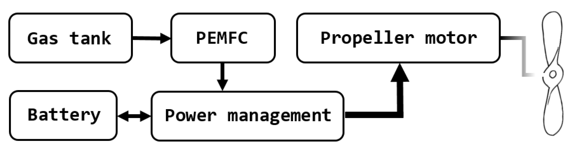
Figure 2.
Polarization curve for a given PEMFC.
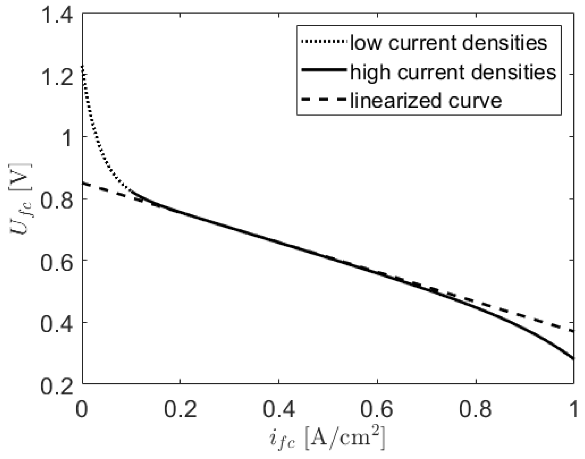
Figure 3.
Time histories of the sUAV climb angle.
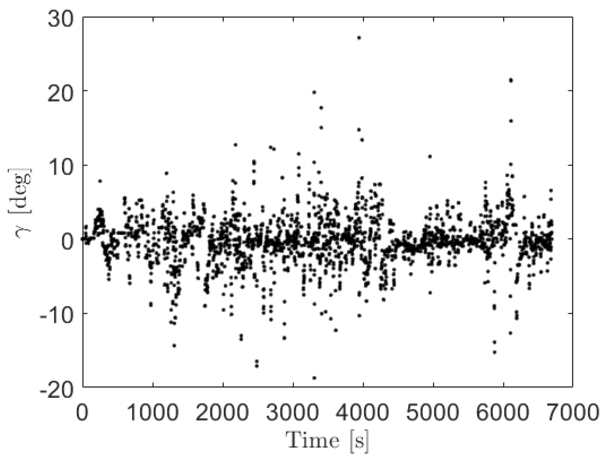
Figure 4.
Time histories of the sUAV motor power.
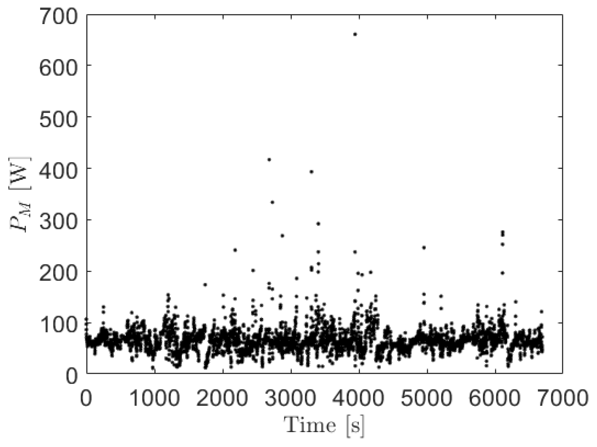
Figure 5.
The effect of the discount factor in the value iteration approach.
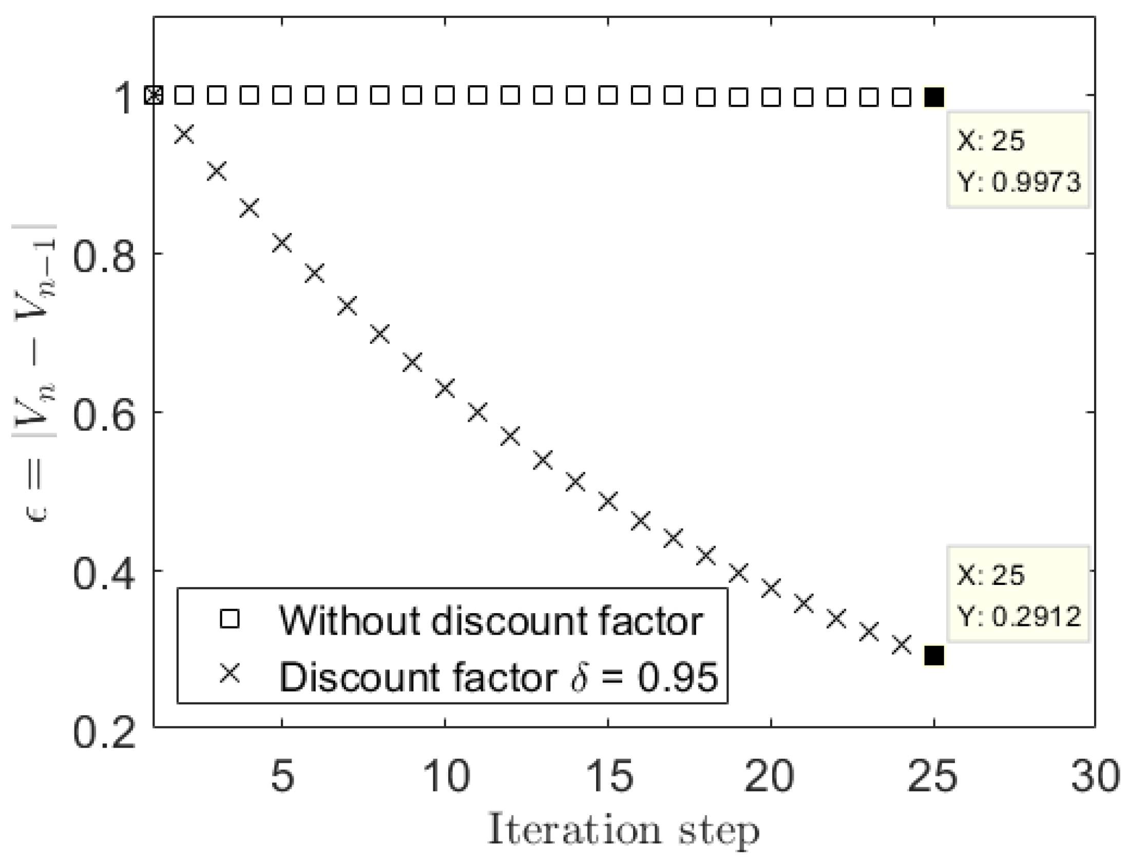
Figure 6.
A cross-section of the control policy in the endurance maximization problem for W and with (a) deg, W, (b) deg, W, (c) deg, W, and (d) deg, W.
Figure 6.
A cross-section of the control policy in the endurance maximization problem for W and with (a) deg, W, (b) deg, W, (c) deg, W, and (d) deg, W.
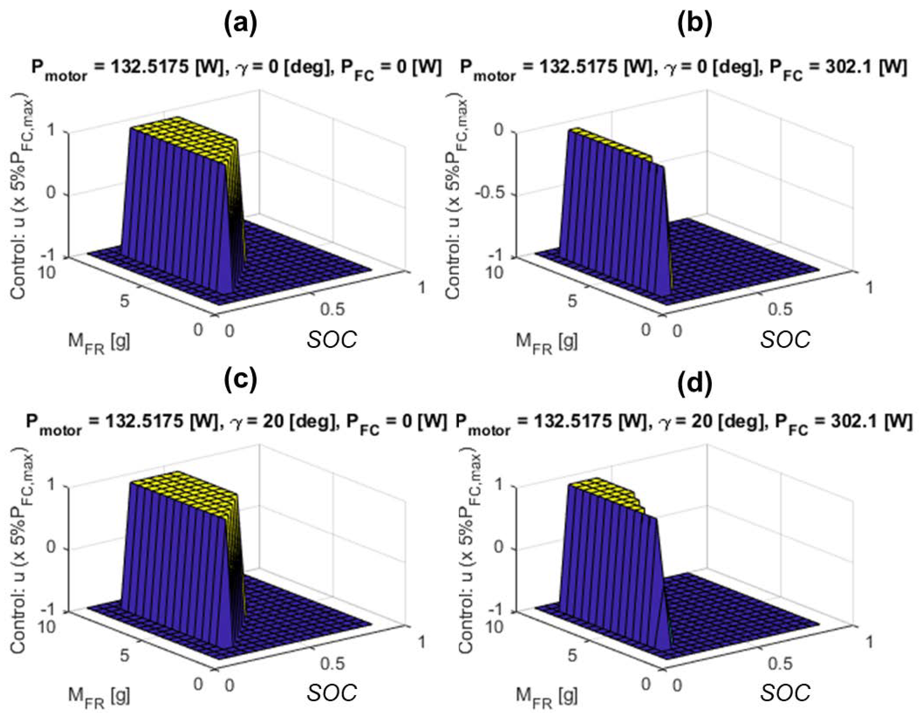
Figure 7.
sUAV and versus time, Simulation Scenario I.
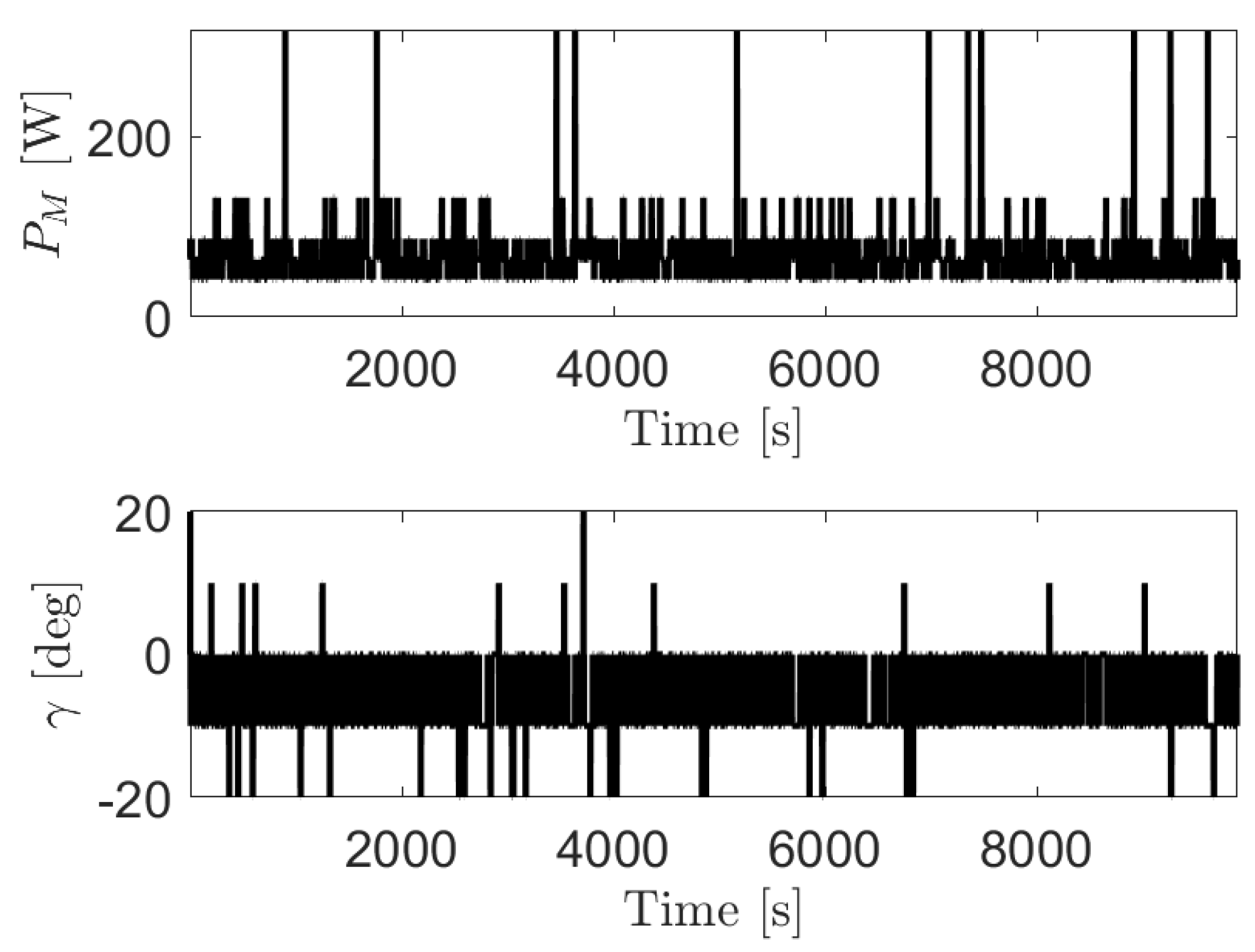
Figure 8.
and remaining versus time, Simulation Scenario I; dashed lines show constraints.
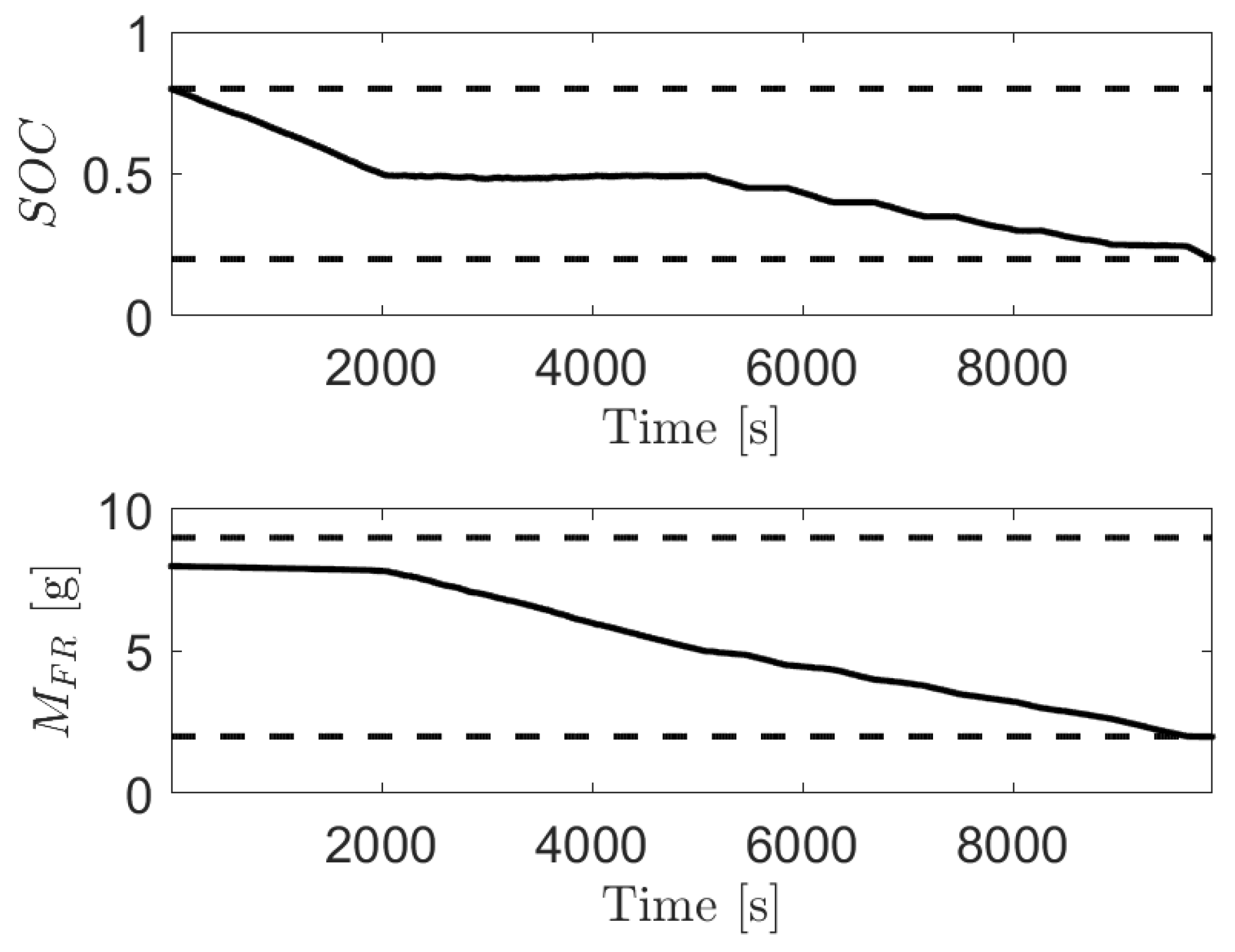
Figure 9.
Fuel cell load demand power and split fraction versus time, Simulation Scenario I. The dashed and dashed-dotted lines in the top sub-figure indicate the maximum with = 0 deg and = 20 deg, respectively.
Figure 9.
Fuel cell load demand power and split fraction versus time, Simulation Scenario I. The dashed and dashed-dotted lines in the top sub-figure indicate the maximum with = 0 deg and = 20 deg, respectively.
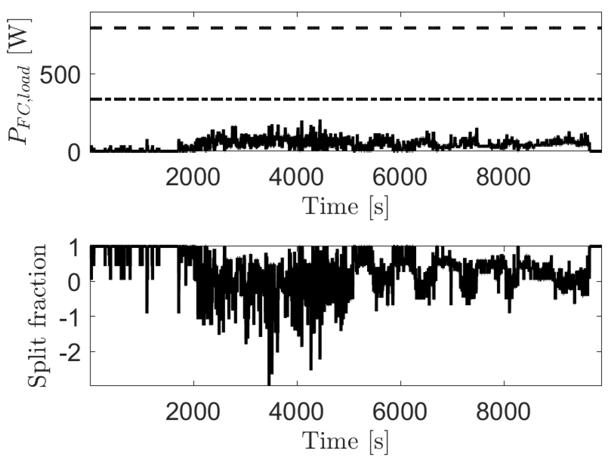
Figure 10.
Battery power, Simulation Scenario I.
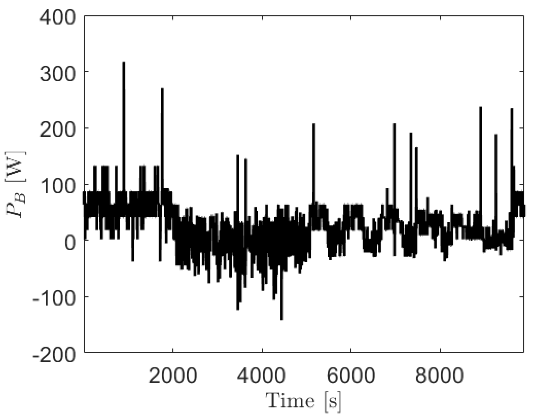
Figure 11.
sUAV and versus time, Simulation Scenario II.
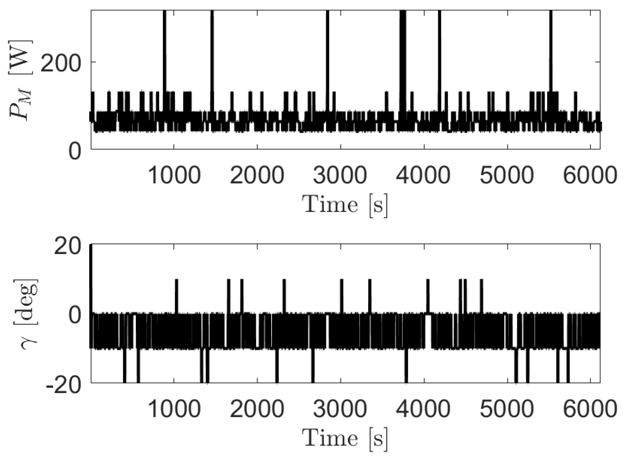
Figure 12.
and remaining versus time, Simulation Scenario II; dashed lines show constraints.
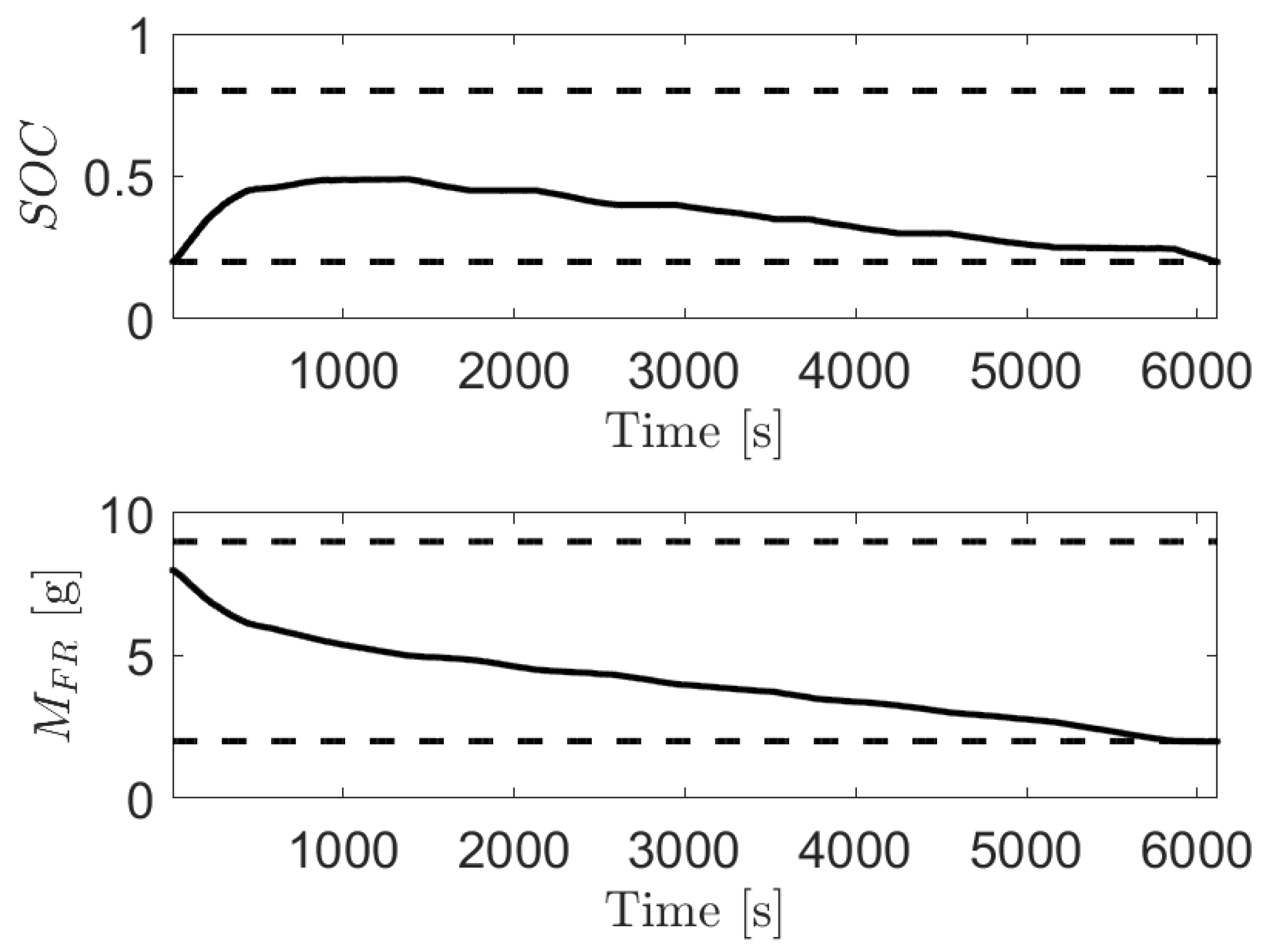
Figure 13.
Fuel cell load demand power and split fraction versus time, Simulation Scenario II. The dashed and dashed-dotted lines in the top figure indicate the maximum with = 0 deg and = 20 deg, respectively.
Figure 13.
Fuel cell load demand power and split fraction versus time, Simulation Scenario II. The dashed and dashed-dotted lines in the top figure indicate the maximum with = 0 deg and = 20 deg, respectively.
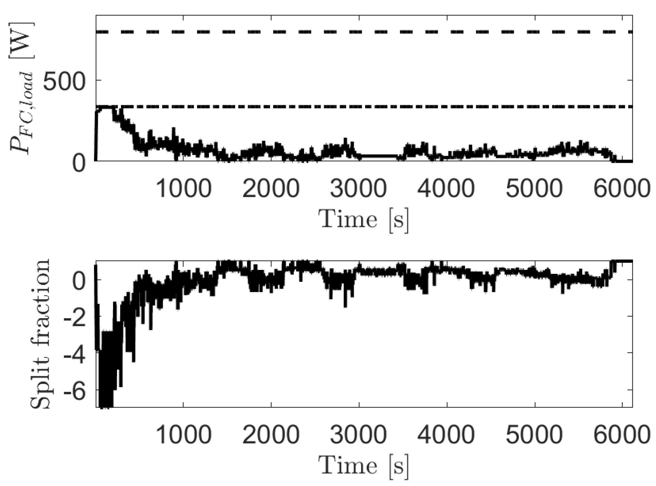
Figure 14.
Battery power, Simulation Scenario II.
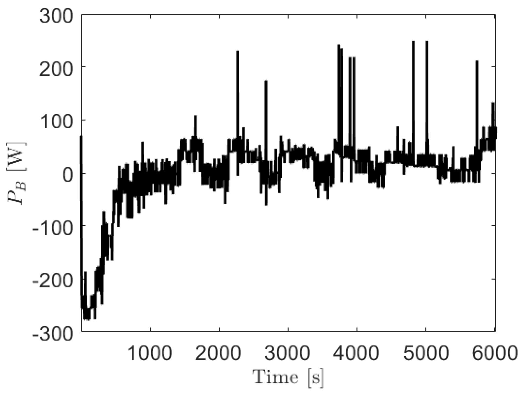
Figure 15.
sUAV and versus time, Simulation Scenario III.
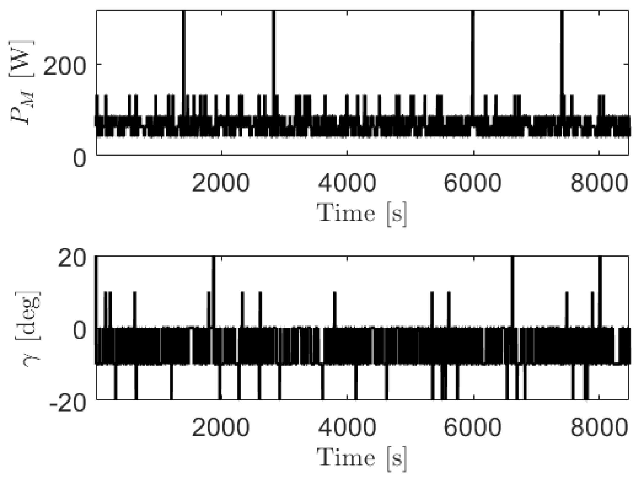
Figure 16.
and remaining versus time, Simulation Scenario III; dashed lines show constraints.
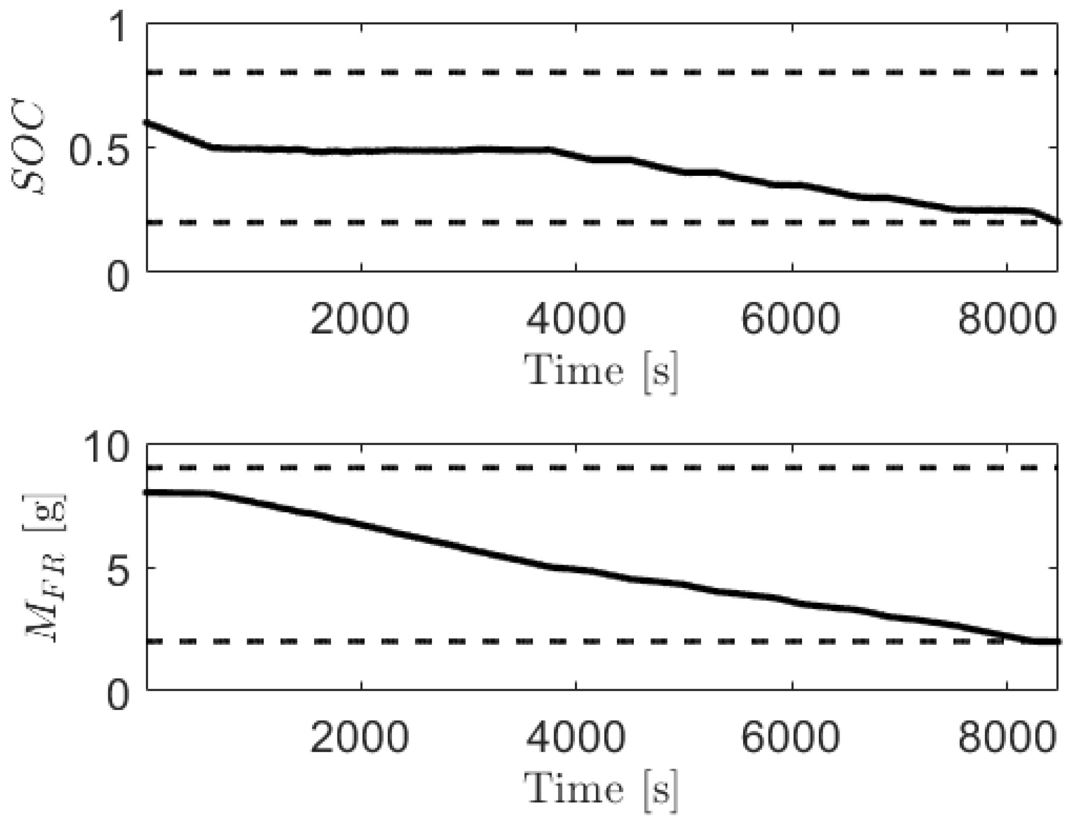
Figure 17.
Fuel cell load demand power and split fraction versus time, Simulation Scenario III. The dashed and dashed-dotted lines in the top figure indicate the maximum with = 0 deg and = 20 deg, respectively.
Figure 17.
Fuel cell load demand power and split fraction versus time, Simulation Scenario III. The dashed and dashed-dotted lines in the top figure indicate the maximum with = 0 deg and = 20 deg, respectively.
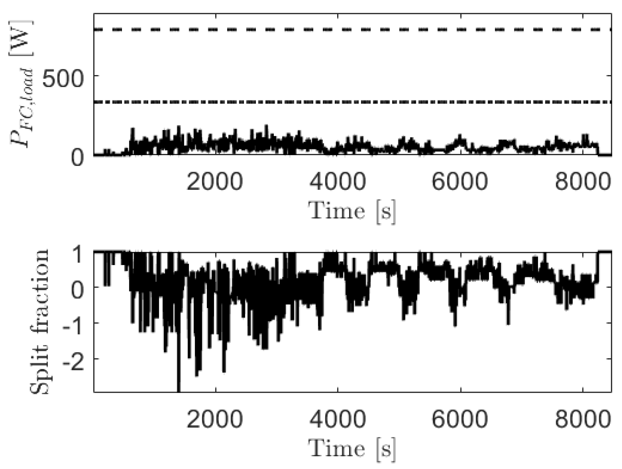
Figure 18.
Battery power, Simulation Scenario III.
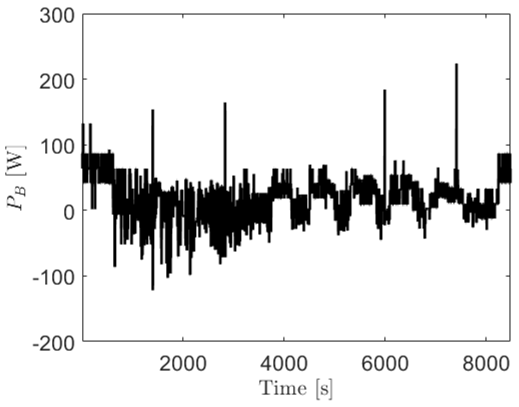
Table 1.
List of variables used in the sUAV model.
| Variable | Description | Unit |
|---|---|---|
| v | Velocity of the sUAV | |
| Climb angle | ||
| T | Thrust force | |
| Angle of attack | ||
| L | Lift force | |
| D | Drag force | |
| sUAV coefficient of lift | ∖ | |
| sUAV coefficient of drag | ∖ | |
| Air density | ||
| Power required by the sUAV | ||
| N | Angular speed of the electric motor | |
| Power generated by the propeller | ||
| Ideal propeller power | ||
| Propulsive efficiency | ∖ | |
| Electric motor driver’s input voltage | ||
| Electric motor driver’s input current | ||
| Elector motor driver’s input power | ||
| Motor efficiency | ∖ | |
| Total power of the fuel cell | ||
| Load demand power of the fuel cell | ||
| Power required by the auxiliaries | ||
| Single cell voltage | ||
| Single cell current | ||
| Single cell current density | ||
| Activation polarization | ||
| Ohmic losses | ||
| Concentration polarization | ||
| Equivalent open circuit voltage of a single fuel cell | ||
| Modified single fuel cell resistance | ||
| Variable defined in Equation (18) | ||
| Open circuit voltage of the battery | ||
| Battery’s state of charge | ∖ | |
| Power of the battery | ||
| Initial SOC | ∖ | |
| Split fraction | ∖ | |
| u | Control input | ∖ |
| Defined in Equation (25) | ||
| Mass of fuel remaining |
Table 2.
Average exit time for different discount factor.
| Number of Iteration | Computing Time (min) | Exit Time with 20% Initial (s) | Exit Time with 80% Initial (s) | |
|---|---|---|---|---|
| 0.99 | 2258 | 830.02 | 6358.44 | 9742.99 |
| 0.97 | 753 | 100.69 | 6276.18 | 9716.86 |
| 0.95 | 448 | 58.27 | 6221.37 | 9640.24 |
| 0.93 | 317 | 39.22 | 6186.50 | 9610.22 |
| 0.91 | 244 | 30.55 | 6159.65 | 9602.55 |
Publisher’s Note: MDPI stays neutral with regard to jurisdictional claims in published maps and institutional affiliations. |
© 2021 by the authors. Licensee MDPI, Basel, Switzerland. This article is an open access article distributed under the terms and conditions of the Creative Commons Attribution (CC BY) license (http://creativecommons.org/licenses/by/4.0/).
Share and Cite
MDPI and ACS Style
Zhang, J.; Kolmanovsky, I.; Amini, M.R. Stochastic Drift Counteraction Optimal Control of a Fuel Cell-Powered Small Unmanned Aerial Vehicle. Energies 2021, 14, 1304. https://doi.org/10.3390/en14051304
AMA Style
Zhang J, Kolmanovsky I, Amini MR. Stochastic Drift Counteraction Optimal Control of a Fuel Cell-Powered Small Unmanned Aerial Vehicle. Energies. 2021; 14(5):1304. https://doi.org/10.3390/en14051304
Chicago/Turabian StyleZhang, Jiadi, Ilya Kolmanovsky, and Mohammad Reza Amini. 2021. "Stochastic Drift Counteraction Optimal Control of a Fuel Cell-Powered Small Unmanned Aerial Vehicle" Energies 14, no. 5: 1304. https://doi.org/10.3390/en14051304
Note that from the first issue of 2016, this journal uses article numbers instead of page numbers. See further details here.