
Solving Single- and Multi-Objective Optimal Reactive Power Dispatch Problems Using an Improved Salp Swarm Algorithm


Abstract
1. Introduction
- (1)
- Solving the ORPD, both as a single- and multi- objective problem, based on a novel optimization technique, namely the salp swarm algorithm.
- (2)
- Improvement of the original algorithm tested on 23 frequently used benchmark functions.
- (3)
- The validity of the proposed model for total power loss reduction and voltage profile enhancement.
2. ORPD Problem Formulation
2.1. Objective Functions
2.1.1. Function 1: Total Active Power Losses
2.1.2. Function 2: Bus Voltage Deviation
2.1.3. Multi-Objective Approach
2.2. Equality Constraints
2.3. Inequality Constraints
2.3.1. Generator Constraints
2.3.2. Capacitor Banks Constraints
2.3.3. OLTC Transformers Constraints
2.3.4. Load Bus Voltage Constraints
2.3.5. Lines Transmission Capacity
3. Model Implementation
3.1. Load Flow Calculation
3.2. Salp Swarm Optimization
3.3. Multi-Objective SSA
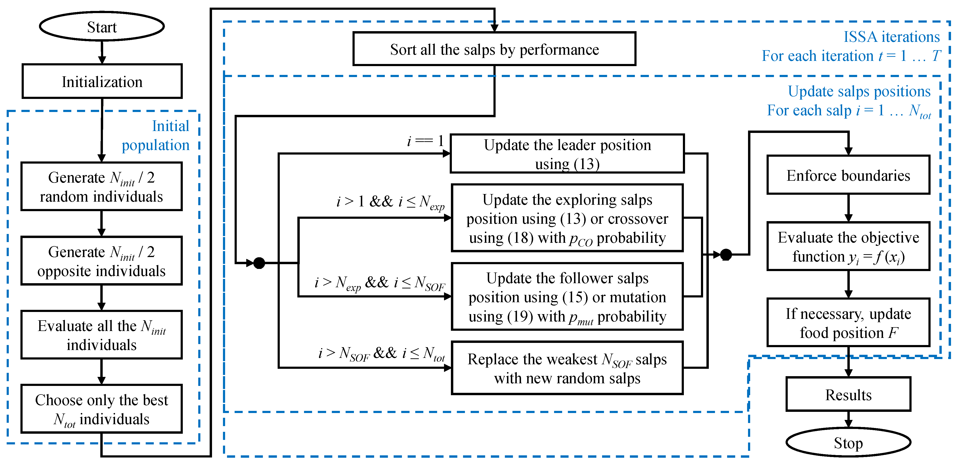
3.4. Proposed Improvements
3.4.1. Opposition-Based Learning Initial Population
3.4.2. Introducing the Exploring Salps and Performance Hierarchy
3.4.3. Crossover
3.4.4. Mutation
3.4.5. Survival of the Fittest
4. Case Study
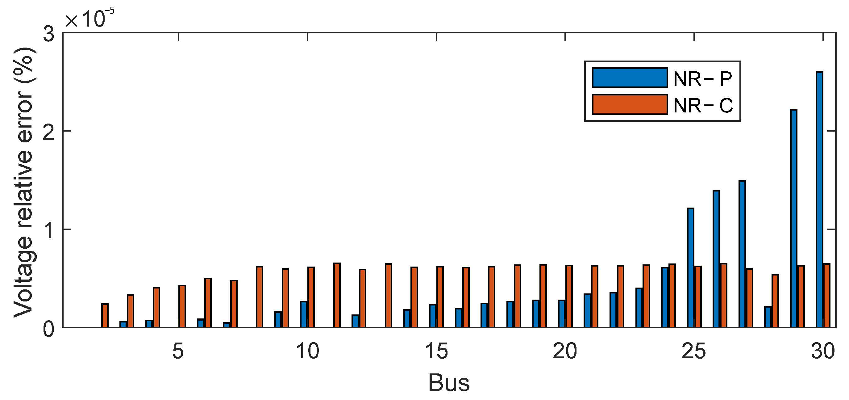
4.1. Load Flow Validation
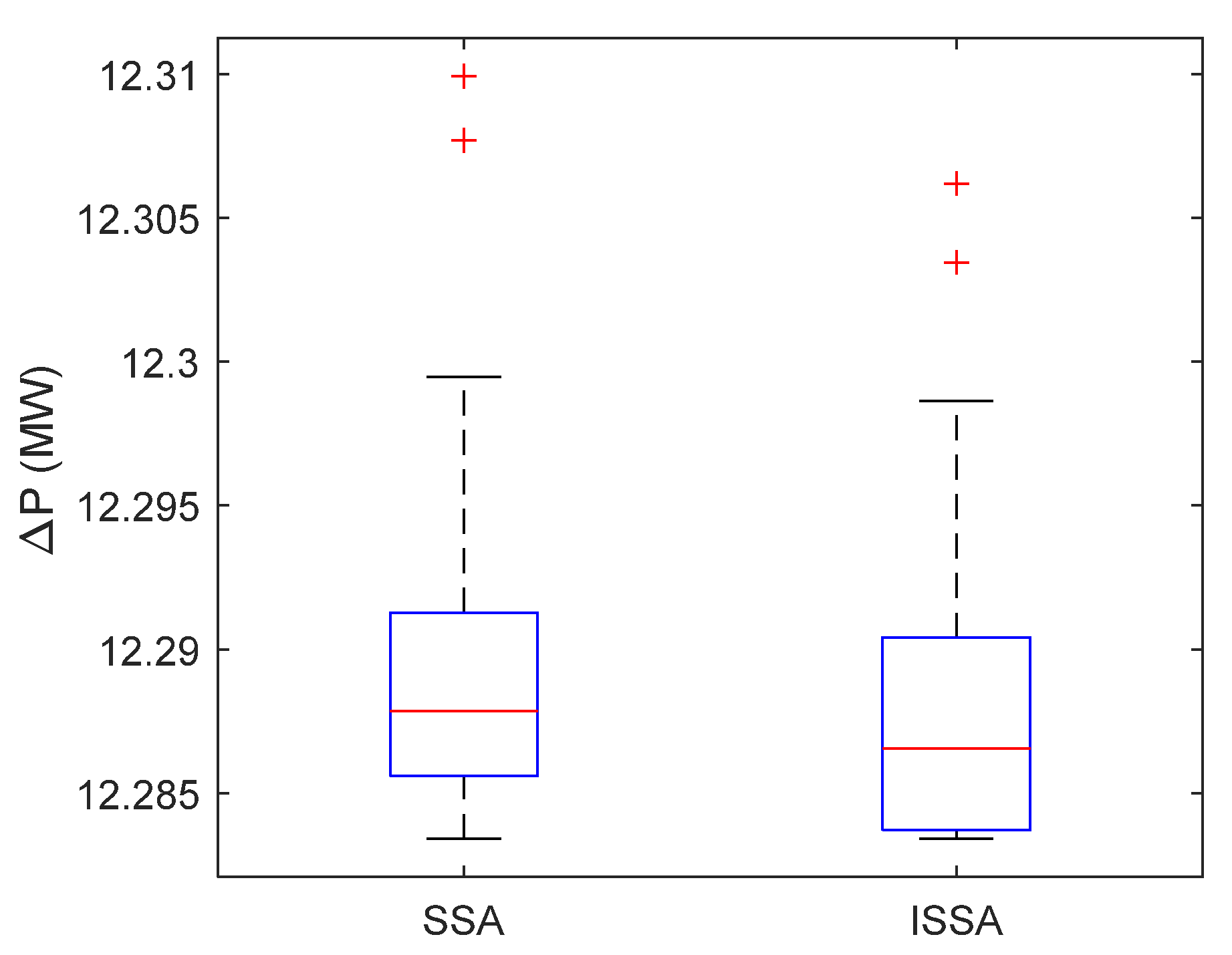
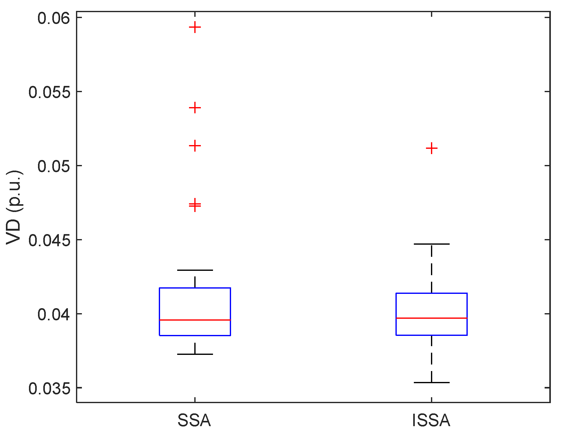
4.2. Conventional SSA vs. ISSA
4.3. Single-Objective ORPD Results
4.3.1. IEEE 14-Bus System
Power Loss Minimization
Voltage Deviation (VD) Minimization
4.3.2. IEEE 30-Bus System
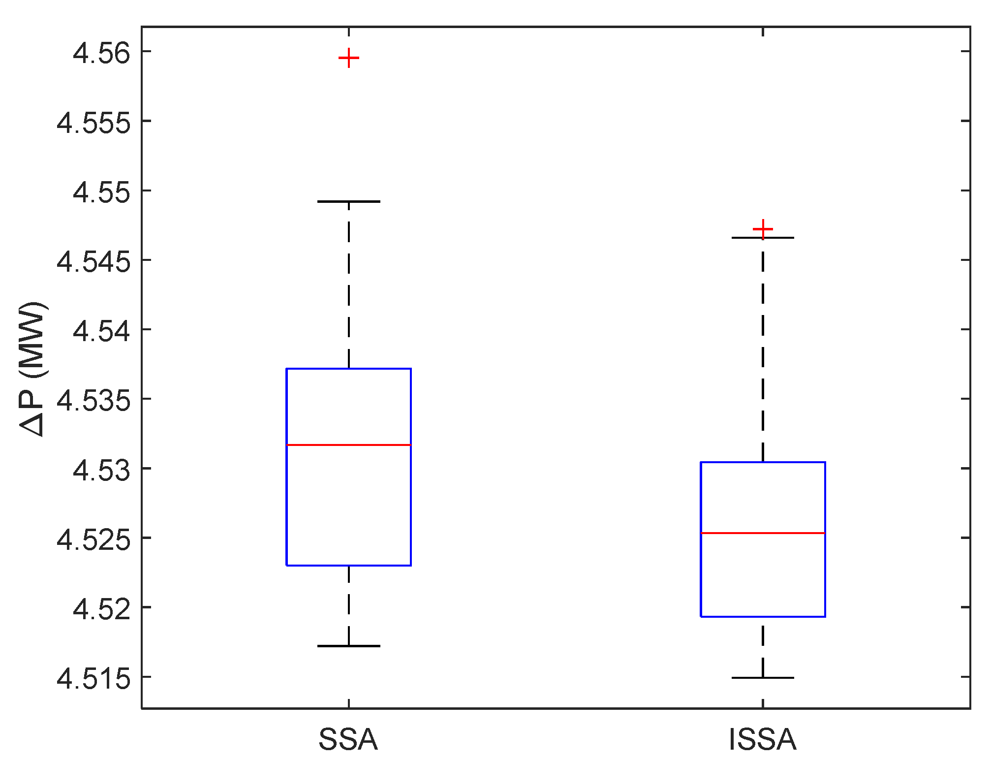
Power Loss Minimization
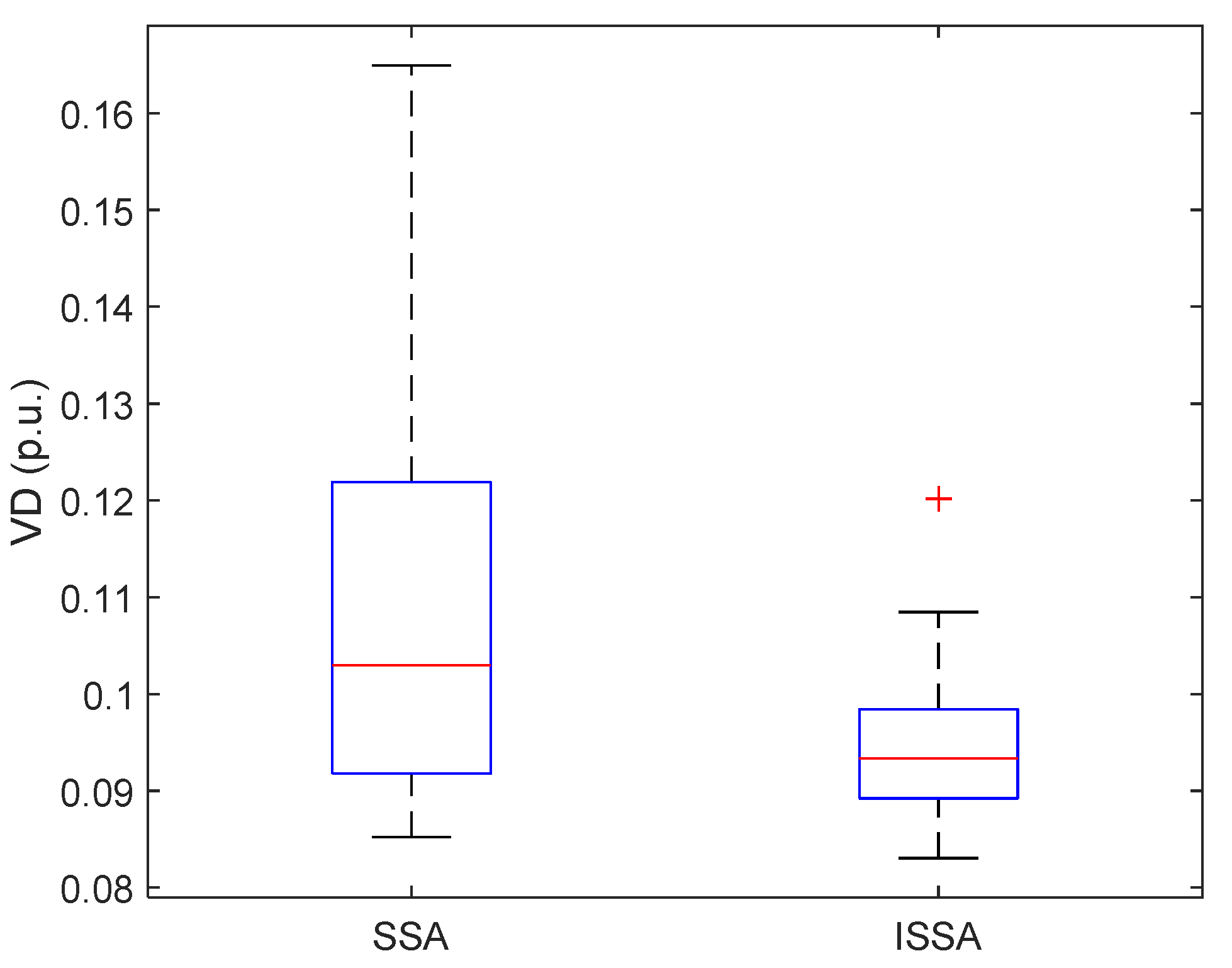
Voltage Deviation (VD) Minimization
4.4. Multi-Objective Approach
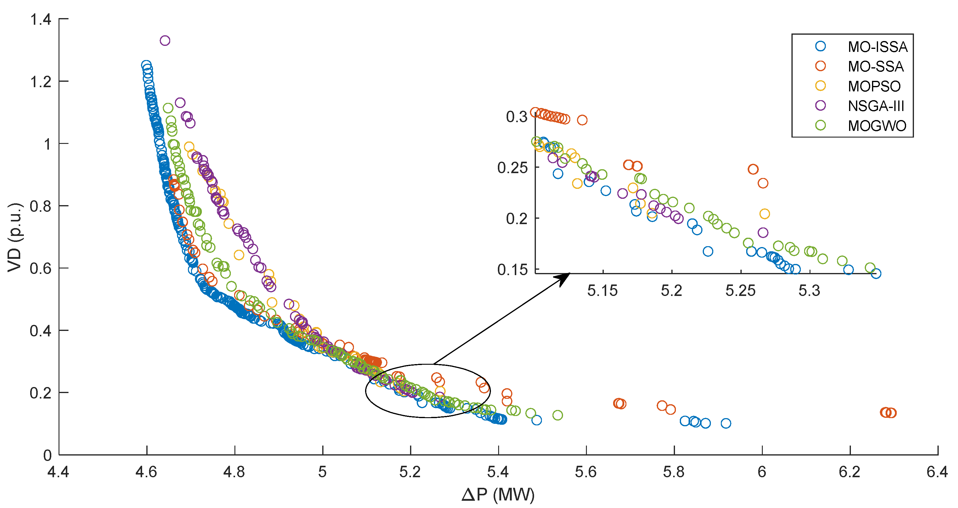
4.4.1. Multi-Objective Optimization on IEEE 14-Bus System
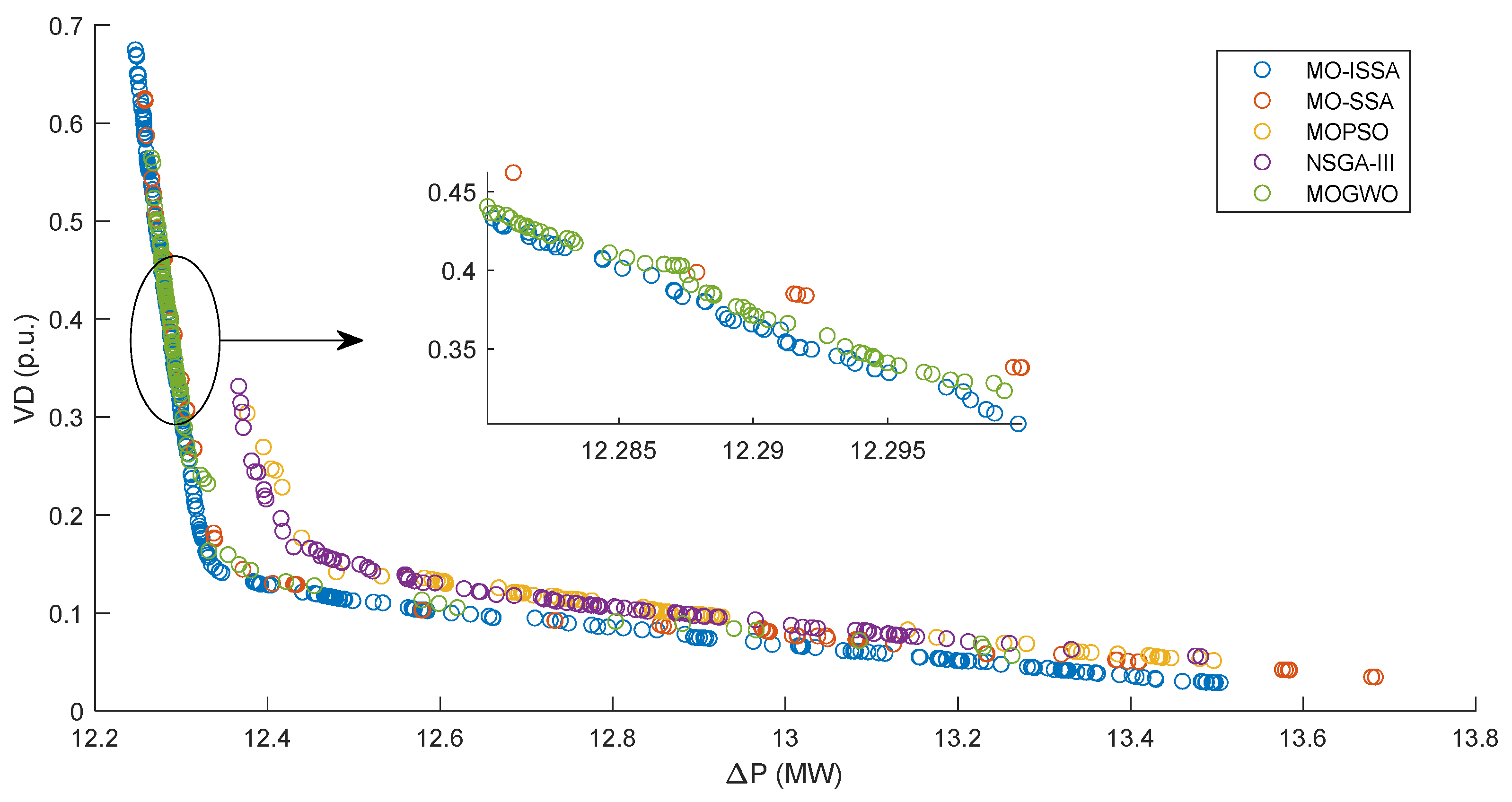
4.4.2. Multi-Objective Optimization on IEEE 30-Bus System
5. Conclusions
Author Contributions
Funding
Conflicts of Interest
References
- Karmakar, N.; Bhattacharyya, B. Optimal reactive power planning in power transmission network using sensitivity based bi-level strategy. Sustain. Energy Grids Netw. 2020, 23, 100383. [Google Scholar] [CrossRef]
- Zeng, Y.; Sun, Y. Application of Hybrid MOPSO Algorithm to Optimal Reactive Power Dispatch Problem Considering Voltage Stability. J. Electr. Comput. Eng. 2014, 2014, 124136. [Google Scholar] [CrossRef]
- Zeng, Y.; Sun, Y. Solving multiobjective optimal reactive power dispatch using improved multiobjective particle swarm optimization. In Proceedings of the 26th Chinese Control and Decision Conference (2014 CCDC), Changsha, China, 31 May–2 June 2014. [Google Scholar]
- Lee, K.Y.; Park, Y.M.; Ortiz, J.L. A United Approach to Optimal Real and Reactive Power Dispatch. IEEE Trans. Power Appar. Syst. 1985, PAS-104, 1147–1153. [Google Scholar] [CrossRef]
- Robbins, B.A.; Dominguez-Garcia, A. Optimal Reactive Power Dispatch for Voltage Regulation in Unbalanced Distribution Systems. IEEE Trans. Power Syst. 2016, 31, 2903–2913. [Google Scholar] [CrossRef]
- Granville, S. Optimal reactive power dispatch through interior point methods. IEEE Trans. Power Syst. 1994, 9, 136–146. [Google Scholar] [CrossRef]
- Sachdeva, S.S.; Billinton, R. Optimum Network Var Planning by Nonlinear Programming. IEEE Trans. Power Appar. Syst. 1973, PAS-92, 1217–1225. [Google Scholar] [CrossRef]
- Pal, B.B.; Biswas, P.; Mukhopadhyay, A. GA Based FGP Approach for Optimal Reactive Power Dispatch. Procedia Technol. 2013, 10, 464–473. [Google Scholar] [CrossRef]
- Duman, S.; Sönmez, Y.; Güvenç, U.; Yörükeren, N. Optimal reactive power dispatch using a gravitational search algorithm. IET Gener. Transm. Distrib. 2012, 6, 563–576. [Google Scholar] [CrossRef]
- Abaci, K.; Yamaçli, V. Optimal reactive-power dispatch using differential search algorithm. Electr. Eng. 2016, 99, 213–225. [Google Scholar] [CrossRef]
- Mei, R.N.S.; Sulaiman, M.H.; Mustaffa, Z.; Daniyal, H. Optimal reactive power dispatch solution by loss minimization using moth-flame optimization technique. Appl. Soft Comput. 2017, 59, 210–222. [Google Scholar]
- Li, X.; Ma, S. Multiobjective Discrete Artificial Bee Colony Algorithm for Multiobjective Permutation Flow Shop Scheduling Problem with Sequence Dependent Setup. IEEE Trans. Eng. Manag. 2017, 64, 149–165. [Google Scholar]
- Kanata, S.; Suwarno, S.; Sianipar, G.H.; Maulidevi, N.U. Non-dominated Sorting Genetic Algorithm III for Multi-objective Optimal Reactive Power Dispatch Problem in Electrical Power System. In Proceedings of the 2nd International Conference on High Voltage Engineering and Power Systems (ICHVEPS), Denpasar, Indonesia, 1–4 October 2019. [Google Scholar]
- Abido, M.A. Multiobjective particle swarm optimization for optimal power flow problem. In Proceedings of the 12th International Middle-East Power System Conference, Aswan, Egypt, 12–15 March 2008. [Google Scholar]
- Abido, M. Multiobjective Optimal VAR Dispatch Using Strength Pareto Evolutionary Algorithm. In Proceedings of the IEEE International Conference on Evolutionary Computation, Vancouver, BC, Canada, 16–21 July 2006. [Google Scholar]
- Mirjalili, S.; Gandomi, A.H.; Mirjalili, S.Z.; Saremi, S.; Faris, H.; Mirjalili, S.M. Salp Swarm Algorithm: A bio-inspired optimizer for engineering design problems. Adv. Eng. Softw. 2017, 114, 163–191. [Google Scholar] [CrossRef]
- Jumani, T.A.; Mustafa, M.W.; Rasid, M.M.; Anjum, W.; Ayub, S. Salp Swarm Optimization Algorithm-Based Controller for Dynamic Response and Power Quality Enhancement of an Islanded Microgrid. Processes 2019, 7, 840. [Google Scholar] [CrossRef]
- Ahmed, A.; Nadeem, M.F.; Sajjad, I.A.; Bo, R.; Khan, I.A. Optimal Allocation of Wind DG with Time Varying Voltage Dependent Loads Using Bio-Inspired: Salp Swarm Algorithm. In Proceedings of the 3rd International Conference on Computing, Mathematics and Engineering Technologies (iCoMET), Sukkur, Pakistan, 29–30 January 2020. [Google Scholar]
- Aprillia, H.; Yang, H.-T.; Huang, C.-M. Short-Term Photovoltaic Power Forecasting Using a Convolutional Neural Network–Salp Swarm Algorithm. Energies 2020, 13, 1879. [Google Scholar] [CrossRef]
- El-sattar, S.A.; Kamel, S.; Ebeed, M.; Jurado, F. An improved version of salp swarm algorithm for solving optimal power flow problem. Soft Comput. 2021. [Google Scholar] [CrossRef]
- Stott, B. Review of load-flow calculation methods. Proc. IEEE 1974, 62, 916–929. [Google Scholar] [CrossRef]
- Sereeter, B.; Vuik, C.; Witteveen, C. On a comparison of Newton–Raphson solvers for power flow problems. J. Comput. Appl. Math. 2019, 360, 157–169. [Google Scholar] [CrossRef]
- Da Costa, V.M.; Martins, N.; Pereira, J.L.R. Developments in the Newton Raphson power flow formulation based on current injections. IEEE Trans. Power Syst. 1999, 14, 1320–1326. [Google Scholar] [CrossRef]
- El Ela, A.A.; Abido, M.; Spea, S. Differential evolution algorithm for optimal reactive power dispatch. Electr. Power Syst. Res. 2011, 81, 458–464. [Google Scholar] [CrossRef]
- Mandal, B.; Roy, P.K. Optimal reactive power dispatch using quasi-oppositional teaching learning based optimization. Electr. Power Energy Syst. 2013, 53, 123–134. [Google Scholar] [CrossRef]
- Sahli, Z.; Hamouda, A.; Bekrar, A.; Trentesaux, D. Reactive Power Dispatch Optimization with Voltage Profile Improvement Using an Efficient Hybrid Algorithm. Energies 2018, 11, 2134. [Google Scholar] [CrossRef]
- Dutta, S.; Roy, P.K.; Nandi, D. Optimal location of STATCOM using chemical reaction optimization for reactive power dispatch problem. Ain Shams Eng. J. 2015, 7, 233–247. [Google Scholar] [CrossRef]
- Abdel-Fatah, S.; Ebeed, M.; Kamel, S. Optimal Reactive Power Dispatch Using Modified Sine Cosine Algorithm. In Proceedings of the International Conference on Innovative Trends in Computer Engineering (ITCE’2019), Aswan, Egypt, 2–4 February 2019. [Google Scholar]
- Ebeed, M.; Alhejji, A.; Kamel, S.; Jurado, F. Solving the Optimal Reactive Power Dispatch Using Marine Predators Algorithm Considering the Uncertainties in Load and Wind-Solar Generation Systems. Energies 2020, 13, 4316. [Google Scholar] [CrossRef]
- Abualigah, L.M.; Alshinwan, M.; Alabool, H. Salp swarm algorithm: A comprehensive survey. Neural Comput. Appl. 2020, 32, 11195–11215. [Google Scholar] [CrossRef]
- Tizhoosh, H. Opposition-Based Learning: A New Scheme for Machine Intelligence. In Proceedings of the International Conference on Computational Intelligence for Modelling, Control and Automation and International Conference on Intelligent Agents, Web Technologies and Internet Commerce (CIMCA-IAWTIC’06), Vienna, Austria, 28–30 November 2005. [Google Scholar]
- Pian, J.; Wang, G.; Li, B. An Improved ABC Algorithm Based on Initial Population and Neighborhood Search. In Proceedings of the 10th IFAC Symposium on Advanced Control of Chemical Processes ADCHEM 2018, Shenyang, China, 25–27 July 2018; Volume 51, pp. 251–256. [Google Scholar]
- Sharapov, R.R. Genetic Algorithms: Basic Ideas, Variants and Analysis. In Vision Systems: Segmentation and Pattern Recognition; IntechOpen: London, UK, 2007. [Google Scholar]
- Wang, J.-S.; Li, S.-X. An Improved Grey Wolf Optimizer Based on Differential Evolution and Elimination Mechanism. Sci. Rep. 2019, 9, 1–21. [Google Scholar] [CrossRef]
- MATPOWER. Available online: https://matpower.org (accessed on 15 December 2020).
- Salp Swarm Algorithm. Available online: https://seyedalimirjalili.com/ssa (accessed on 15 December 2020).
- Power Systems Test Case Archive. Available online: http://labs.ece.uw.edu/pstca/ (accessed on 1 February 2020).
- Chen, G.; Liu, L.; Zhang, Z.; Huang, S. Optimal reactive power dispatch by improved GSA-based algorithm with the novel strategies to handle constraints. Appl. Soft Comput. 2017, 50, 58–70. [Google Scholar] [CrossRef]
- Vishnu, M.; Sunil Kumar, T.K. An Improved Solution for Reactive Power Dispatch Problem Using Diversity-Enhanced Particle Swarm Optimization. Energies 2020, 13, 2862. [Google Scholar] [CrossRef]
- Deb, K.; Jain, H. An Evolutionary Many-Objective Optimization Algorithm Using Reference-Point-Based Nondominated Sorting Approach, Part I: Solving Problems with Box Constraints. IEEE Trans. Evol. Comput. 2014, 18, 577–601. [Google Scholar] [CrossRef]
- Mostapha Kalami Heris, Multi-Objective PSO in MATLAB. Available online: https://yarpiz.com/59/ypea121-mopso (accessed on 2 February 2021).
- Mirjalili, S.; Saremi, S.; Mirjalili, S.M.; Coelho, L. Multi-objective grey wolf optimizer: A novel algorithm for multi-criterion optimization. Expert Syst. Appl. 2016, 47, 106–119. [Google Scholar] [CrossRef]


| i ≠ j | i = j |
|---|---|
| Benchmark Function | Best | Average | Worst | Std. Dev. | ||||
|---|---|---|---|---|---|---|---|---|
| ISSA | SSA | ISSA | SSA | ISSA | SSA | ISSA | SSA | |
| F1 | 5.64 × 10⁻¹³ | 5.15 × 10⁻⁹ | 6.38 × 10⁻¹² | 6.96 × 10⁻⁹ | 1.45 × 10⁻¹¹ | 1.05 × 10⁻⁸ | 4.02 × 10⁻¹² | 1.21 × 10⁻⁹ |
| F2 | 1.18 × 10⁻⁷ | 3.68 × 10⁻⁶ | 3.08 × 10⁻⁷ | 5.48 × 10⁻⁶ | 5.72 × 10⁻⁷ | 8.03 × 10⁻⁶ | 1.10 × 10⁻⁷ | 9.74 × 10⁻⁷ |
| F3 | 8.90 × 10⁻¹⁴ | 1.83 × 10⁻¹⁰ | 2.53 × 10⁻¹² | 4.35 × 10⁻¹⁰ | 6.48 × 10⁻¹² | 8.45 × 10⁻¹⁰ | 1.72 × 10⁻¹² | 1.94 × 10⁻¹⁰ |
| F4 | 1.32 × 10⁻⁷ | 6.45 × 10⁻⁶ | 6.71 × 10⁻⁷ | 1.19 × 10⁻⁵ | 1.55 × 10⁻⁶ | 1.74 × 10⁻⁵ | 3.81 × 10⁻⁷ | 2.33 × 10⁻⁶ |
| F5 | 2.587318 | 0.011634 | 4.110208 | 117.4396 | 4.858855 | 1183.956 | 0.429069 | 244.1039 |
| F6 | 2.16 × 10⁻¹⁰ | 1.72 × 10⁻¹⁰ | 3.19 × 10⁻¹⁰ | 4.50 × 10⁻¹⁰ | 5.01 × 10⁻¹⁰ | 7.88 × 10⁻¹⁰ | 7.59 × 10⁻¹¹ | 1.65 × 10⁻¹⁰ |
| F7 | 1.08 × 10⁻⁶ | 0.000552 | 2.23 × 10⁻⁵ | 0.002002 | 8.94 × 10⁻⁵ | 0.005095 | 2.38 × 10⁻⁵ | 0.001264 |
| F8 | −3854.25 | −3617.37 | −2877.61 | −3052.87 | −2402.63 | −2531.64 | 329.3672 | 316.8193 |
| F9 | 1.28 × 10⁻¹³ | 9.949586 | 1.01 × 10⁻¹² | 22.85084 | 3.01 × 10⁻¹² | 44.77286 | 7.44 × 10⁻¹³ | 9.469586 |
| F10 | 1.91 × 10⁻⁷ | 7.44 × 10⁻⁶ | 4.79 × 10⁻⁷ | 0.810233 | 1.06 × 10⁻⁶ | 2.316849 | 1.99 × 10⁻⁷ | 0.817508 |
| F11 | 4.46 × 10⁻¹³ | 0.132949 | 5.91 × 10⁻¹² | 0.33718 | 2.84 × 10⁻¹¹ | 0.693639 | 6.39 × 10⁻¹² | 0.14227 |
| F12 | 8.13 × 10⁻¹³ | 9.42 × 10⁻¹³ | 2.56 × 10⁻¹² | 0.051897 | 3.99 × 10⁻¹² | 0.62195 | 7.46 × 10⁻¹³ | 0.143383 |
| F13 | 2.42 × 10⁻¹² | 4.49 × 10⁻¹² | 0.000366 | 0.001099 | 0.010987 | 0.010987 | 0.002006 | 0.003353 |
| F14 | 0.998004 | 0.998004 | 0.998004 | 0.998004 | 0.998004 | 0.998004 | 1.62 × 10⁻¹⁶ | 2.31 × 10⁻¹⁶ |
| F15 | 0.000307 | 0.000618 | 0.000307 | 0.000829 | 0.000307 | 0.001223 | 3.41 × 10⁻¹⁴ | 0.000204 |
| F16 | −1.03163 | −1.03163 | −1.03163 | −1.03163 | −1.03163 | −1.03163 | 8.04 × 10⁻¹⁶ | 5.80 × 10⁻¹⁵ |
| F17 | 0.397887 | 0.397887 | 0.397887 | 0.397887 | 0.397887 | 0.397887 | 7.99 × 10⁻¹⁶ | 1.33 × 10⁻¹⁴ |
| F18 | 3 | 3 | 3 | 3 | 3 | 3 | 1.38 × 10⁻¹⁴ | 7.38 × 10⁻¹⁴ |
| F19 | −3.86278 | −3.86278 | −3.86278 | −3.86278 | −3.86278 | −3.86278 | 1.61 × 10⁻¹⁵ | 5.99 × 10⁻¹⁵ |
| F20 | −3.322 | −3.322 | −3.23084 | −3.21497 | −3.2031 | −3.20301 | 0.051146 | 0.036284 |
| F21 | −10.1532 | −10.1532 | −10.1532 | −8.80506 | −10.1532 | −2.63047 | 4.91 × 10⁻¹² | 2.543965 |
| F22 | −10.4029 | −10.4029 | −10.0486 | −8.46635 | −5.08767 | −5.08767 | 1.348527 | 2.588702 |
| F23 | −10.5364 | −10.5364 | −10.5364 | −9.28557 | −10.5364 | −5.17565 | 3.47 × 10⁻¹² | 2.30611 |
| Control variable | QG2 [p.u.] | QG3 [p.u.] | QG6 [p.u.] | QG8 [p.u.] | Transformers Tap [p.u.] | Capacitor Bank [p.u.] |
|---|---|---|---|---|---|---|
| Min. | −0.4 | 0 | −0.06 | −0.06 | 0.9 | 0 |
| Max. | 0.5 | 0.4 | 0.24 | 0.24 | 1.1 | 0.18 |
| Control Variables | GSA | PSO | IGSA | DEPSO | JAYA | SSA | ISSA | |
|---|---|---|---|---|---|---|---|---|
| Bus voltages (p.u) | V1 | 1.1 | 1.1 | 1.1 | 1.019 | 0.959 | 1.1 | 1.1 |
| V2 | 1.076398 | 1.077022 | 1.076578 | 1.0393 | 0.9604 | 1.085801 | 1.085802 | |
| V3 | 1.052355 | 1.046782 | 1.046787 | 0.9817 | 0.9664 | 1.05631 | 1.056346 | |
| V6 | 1.008185 | 1.020621 | 1.062305 | 1.0246 | 1.0389 | 1.096912 | 1.096919 | |
| V8 | 1.049006 | 1.071699 | 1.097861 | 1.0015 | 1.0019 | 1.1 | 1.1 | |
| Transformer tap ratio (p.u.) | T1 | 1.04 | 1.02 | 1.02 | 1.03 | 1.0451 | 1.03 | 1.03 |
| T2 | 1.02 | 1 | 0.94 | 0.95 | 0.9733 | 0.9 | 0.9 | |
| T3 | 1 | 1.04 | 1 | 1.03 | 1.0135 | 0.98 | 0.98 | |
| Capacitor bank (p.u.) | Q9 | 0.035 | 0 | 0.05 | 0.14 | 0.15 | 0.18 | 0.18 |
| Power Losses (MW) | 12.64782 | 12.46588 | 12.39706 | 13.4086 | 13.466 | 12.2834 | 12.2834 | |
| GSA | PSO | IGSA | DEPSO | JAYA | SSA | ISSA | |
|---|---|---|---|---|---|---|---|
| Min. ∆P | 12.64782 | 12.46588 | 12.39706 | 13.4086 | 13.466 | 12.2834 | 12.2834 |
| Avg. ∆P | 13.21897 | 12.78373 | 12.46443 | - | - | 12.2899 | 12.2885 |
| Max. ∆P | 14.36926 | 13.67714 | 12.90281 | - | - | 12.3099 | 12.3062 |
| Std. dev. ∆P | 0.52 | 0.38 | 0.094 | - | - | 0.0066 | 0.0061 |
| Control Variables | GSA | PSO | IGSA | SSA | ISSA | |
|---|---|---|---|---|---|---|
| Bus voltages (p.u) | V1 | 1.061589 | 1.061683 | 1.060879 | 1.1 | 1.036251 |
| V2 | 1.035651 | 1.042381 | 1.040856 | 1.033085 | 1.007634 | |
| V3 | 0.99018 | 1.013994 | 1.011222 | 0.989761 | 1.021722 | |
| V6 | 1.024779 | 1.023954 | 1.016776 | 1.0198 | 1.036232 | |
| V8 | 1.030956 | 1.018293 | 1.035129 | 1.026928 | 1.073828 | |
| Transformer tap ratio (p.u.) | T1 | 1.04 | 1.1 | 1.04 | 1.04 | 1.04 |
| T2 | 0.94 | 0.9 | 0.9 | 0.93 | 0.92 | |
| T3 | 0.96 | 0.9 | 0.92 | 0.92 | 0.91 | |
| Capacitor Bank (p.u.) | Q9 | 0.03 | 0.05 | 0.05 | 0.17 | 0.07 |
| Voltage deviation (p.u.) | 0.06727 | 0.08808 | 0.0339 | 0.0373 | 0.0353 | |
| GSA | PSO | IGSA | SSA | ISSA | |
|---|---|---|---|---|---|
| Min. VD | 0.06727 | 0.08808 | 0.0339 | 0.0373 | 0.0353 |
| Avg. VD | 0.1791 | 0.18294 | 0.04583 | 0.0415 | 0.0404 |
| Max. VD | 0.30376 | 0.27049 | 0.09056 | 0.0594 | 0.0512 |
| Std. dev. VD | 0.066 | 0.0603 | 0.017 | 0.0052 | 0.003 |
| Control Variable | QG2 [p.u.] | QG5 [p.u.] | QG8 [p.u.] | QG11 [p.u.] | QG13 [p.u.] | Transformers Tap [p.u.] | Capacitor Banks [p.u.] |
|---|---|---|---|---|---|---|---|
| Min. | −0.2 | −0.15 | −0.15 | −0.10 | −0.15 | 0.9 | 0 |
| Max. | 1 | 0.8 | 0.6 | 0.5 | 0.6 | 1.1 | 0.05 |
| Control Variables | MPA | PSO-TS | CRO | QOTLBO | DE | MSCA | SSA | ISSA | |
|---|---|---|---|---|---|---|---|---|---|
| Bus voltages (p.u) | V1 | 1.1 | 1.1 | 1.0998 | 1.1 | 1.1 | 1.1 | 1.1 | 1.1 |
| V2 | 1.0949 | 1.0943 | 1.0939 | 1.0942 | 1.0931 | 1.0945 | 1.0941 | 1.0944 | |
| V5 | 1.0761 | 1.0749 | 1.0743 | 1.0745 | 1.0736 | 1.0753 | 1.0746 | 1.0749 | |
| V8 | 1.078 | 1.0766 | 1.0762 | 1.0765 | 1.0756 | 1.0769 | 1.0765 | 1.0766 | |
| V11 | 1.0873 | 1.1 | 1.0997 | 1.1 | 1.1 | 1.1 | 1.1 | 1.1 | |
| V13 | 1.1 | 1.1 | 1.0999 | 1.0999 | 1.1 | 1.1 | 1.1 | 1.1 | |
| Transformer tap ratio (p.u.) | T1 | 0.9807 | 0.9744 | 0.9765 | 1.0251 | 1.0465 | 1.0355 | 1.0262 | 1.0466 |
| T2 | 1.0222 | 1.051 | 0.9574 | 0.9439 | 0.9097 | 0.9063 | 0.9039 | 0.9 | |
| T3 | 0.9765 | 0.9 | 0.9748 | 0.9992 | 0.9867 | 0.98591 | 0.9784 | 0.9761 | |
| T4 | 0.9707 | 0.9635 | 0.9546 | 0.9732 | 0.9689 | 0.9679 | 0.9655 | 0.9639 | |
| Capacitor Bank Reactive Power Output (p.u.) | Q10 | 0.0179 | 0.05 | 0.0499 | 0.05 | 0.05 | 0.0499 | 0.0291 | 0.05 |
| Q12 | 0.0483 | 0.05 | 0.0499 | 0.05 | 0.05 | 0.0499 | 0.05 | 0.0389 | |
| Q15 | 0.0397 | 0.05 | 0.0499 | 0.05 | 0.05 | 0.04949 | 0.0406 | 0.043 | |
| Q17 | 0.0499 | 0.05 | 0.0499 | 0.05 | 0.05 | 0.05 | 0.05 | 0.05 | |
| Q20 | 0.0422 | 0.0386 | 0.0422 | 0.0445 | 0.04406 | 0.0487 | 0.0356 | 0.0428 | |
| Q21 | 0.0461 | 0.05 | 0.0499 | 0.05 | 0.05 | 0.0499 | 0.05 | 0.05 | |
| Q23 | 0.0469 | 0.05 | 0.0263 | 0.0283 | 0.028004 | 0.0397 | 0.0353 | 0.0316 | |
| Q24 | 0.0412 | 0.05 | 0.05 | 0.05 | 0.05 | 0.05 | 0.05 | 0.05 | |
| Q29 | 0.0329 | 0.0213 | 0.0228 | 0.0256 | 0.025979 | 0.0251 | 0.0251 | 0.0211 | |
| Power Losses (MW) | 4.5335 | 4.5213 | 4.5322 | 4.5594 | 4.555 | 4.5399 | 4.5172 | 4.5149 | |
| MPA | PSO-TS | CRO | QOTLBO | DE | MSCA | SSA | ISSA | |
|---|---|---|---|---|---|---|---|---|
| Min. ∆P | 4.5335 | 4.5213 | 4.5322 | 4.5594 | 4.555 | 4.5399 | 4.5172 | 4.5149 |
| Avg. ∆P | 4.55389 | - | 4.5413 | 4.5601 | - | 4.5518 | 4.5317 | 4.5269 |
| Max. ∆P | 4.6006 | - | 4.5476 | 4.5617 | - | 4.5768 | 4.5595 | 4.5472 |
| Std. dev. ∆P | - | - | - | 0.037 | - | - | 0.0110 | 0.0088 |
| Control Variables | MPA | PSO-TS | CRO | QOTLBO | DE | MSCA | SSA | ISSA | |
|---|---|---|---|---|---|---|---|---|---|
| Bus voltages (p.u) | V1 | 0.9971 | 0.9867 | 1.0089 | 1.0005 | 1.01 | 1.0574 | 1.0054 | 0.9793 |
| V2 | 0.9959 | 0.991 | 1.0044 | 0.9919 | 0.9918 | 1.015 | 1.0039 | 1 | |
| V5 | 1.0164 | 1.0244 | 1.0218 | 1.0217 | 1.0179 | 1.0129 | 1 | 1.0042 | |
| V8 | 0.9971 | 1.0042 | 1.0041 | 1.0147 | 1.0183 | 1.0047 | 1.0005 | 0.9996 | |
| V11 | 1.0387 | 1.0106 | 1.0027 | 0.995 | 1.0114 | 1.0431 | 1.0837 | 1.0966 | |
| V13 | 1.0251 | 1.0734 | 1.0284 | 1.0447 | 1.0282 | 1.0072 | 1.0294 | 1.0684 | |
| Transformer tap ratio (p.u.) | T1 | 1.0556 | 1.0725 | 1.0142 | 1.0076 | 1.0265 | 1.0574 | 1.0847 | 1.0765 |
| T2 | 1.018 | 0.9797 | 0.9004 | 0.903 | 0.9038 | 0.9134 | 0.9092 | 0.9341 | |
| T3 | 1.023 | 0.9273 | 1.0136 | 1.0472 | 1.0114 | 0.9668 | 0.9952 | 1.0869 | |
| T4 | 0.9676 | 0.9607 | 0.9667 | 0.9674 | 0.9635 | 0.9649 | 0.9339 | 0.9354 | |
| Capacitor Bank Reactive Power Output (p.u.) | Q10 | 0.045 | 0.0095 | 0.05 | 0.0487 | 0.0494 | 0.0499 | 0.0172 | 0.0343 |
| Q12 | 0.0497 | 0.0215 | 0.0199 | 0.0304 | 0.0109 | 0.0002 | 0.0097 | 0.0488 | |
| Q15 | 0.0499 | 0.0226 | 0.0498 | 0.05 | 0.05 | 0.0378 | 0.0127 | 0.0182 | |
| Q17 | 0.024 | 0.0005 | 0 | 0 | 0.0024 | 0.0173 | 0.0364 | 0.0118 | |
| Q20 | 0.0463 | 0.0359 | 0.05 | 0.05 | 0.05 | 0.0499 | 0.0345 | 0.0459 | |
| Q21 | 0.0499 | 0.0401 | 0.0499 | 0.05 | 0.0491 | 0.0499 | 0.0424 | 0.0487 | |
| Q23 | 0.0426 | 0.0427 | 0.05 | 0.05 | 0.0499 | 0.0481 | 0.0458 | 0.0364 | |
| Q24 | 0.0499 | 0.0374 | 0.05 | 0.05 | 0.0497 | 0.05 | 0.0378 | 0.0244 | |
| Q29 | 0.0193 | 0.021 | 0.0497 | 0.0256 | 0.0223 | 0.0222 | 0.0099 | 0.0113 | |
| Voltage Deviation (p.u.) | 0.08514 | 0.0866 | 0.0849 | 0.0856 | 0.0911 | 0.097 | 0.0854 | 0.0831 | |
| MPA | PSO-TS | CRO | QOTLBO | DE | MSCA | SSA | ISSA | |
|---|---|---|---|---|---|---|---|---|
| Min. VD | 0.08513 | 0.0866 | 0.0849 | 0.0856 | 0.0911 | 0.097 | 0.0854 | 0.0831 |
| Avg. VD | 0.09454 | - | 0.0863 | 0.0872 | - | 0.1019 | 0.1088 | 0.0947 |
| Max. VD | 0.099 | - | 0.0898 | 0.0907 | - | 0.138 | 0.1649 | 0.1202 |
| Std. dev. VD | - | - | - | 0.0314 | - | - | 0.0207 | 0.0080 |
Publisher’s Note: MDPI stays neutral with regard to jurisdictional claims in published maps and institutional affiliations. |
© 2021 by the authors. Licensee MDPI, Basel, Switzerland. This article is an open access article distributed under the terms and conditions of the Creative Commons Attribution (CC BY) license (http://creativecommons.org/licenses/by/4.0/).
Share and Cite
Tudose, A.M.; Picioroaga, I.I.; Sidea, D.O.; Bulac, C. Solving Single- and Multi-Objective Optimal Reactive Power Dispatch Problems Using an Improved Salp Swarm Algorithm. Energies 2021, 14, 1222. https://doi.org/10.3390/en14051222
Tudose AM, Picioroaga II, Sidea DO, Bulac C. Solving Single- and Multi-Objective Optimal Reactive Power Dispatch Problems Using an Improved Salp Swarm Algorithm. Energies. 2021; 14(5):1222. https://doi.org/10.3390/en14051222
Chicago/Turabian StyleTudose, Andrei M., Irina I. Picioroaga, Dorian O. Sidea, and Constantin Bulac. 2021. "Solving Single- and Multi-Objective Optimal Reactive Power Dispatch Problems Using an Improved Salp Swarm Algorithm" Energies 14, no. 5: 1222. https://doi.org/10.3390/en14051222
APA StyleTudose, A. M., Picioroaga, I. I., Sidea, D. O., & Bulac, C. (2021). Solving Single- and Multi-Objective Optimal Reactive Power Dispatch Problems Using an Improved Salp Swarm Algorithm. Energies, 14(5), 1222. https://doi.org/10.3390/en14051222