
A Novel Procedure for Coupled Simulation of Thermal and Fluid Flow Models for Rough-Walled Rock Fractures


Abstract

1. Introduction
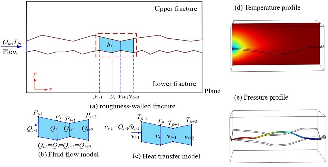
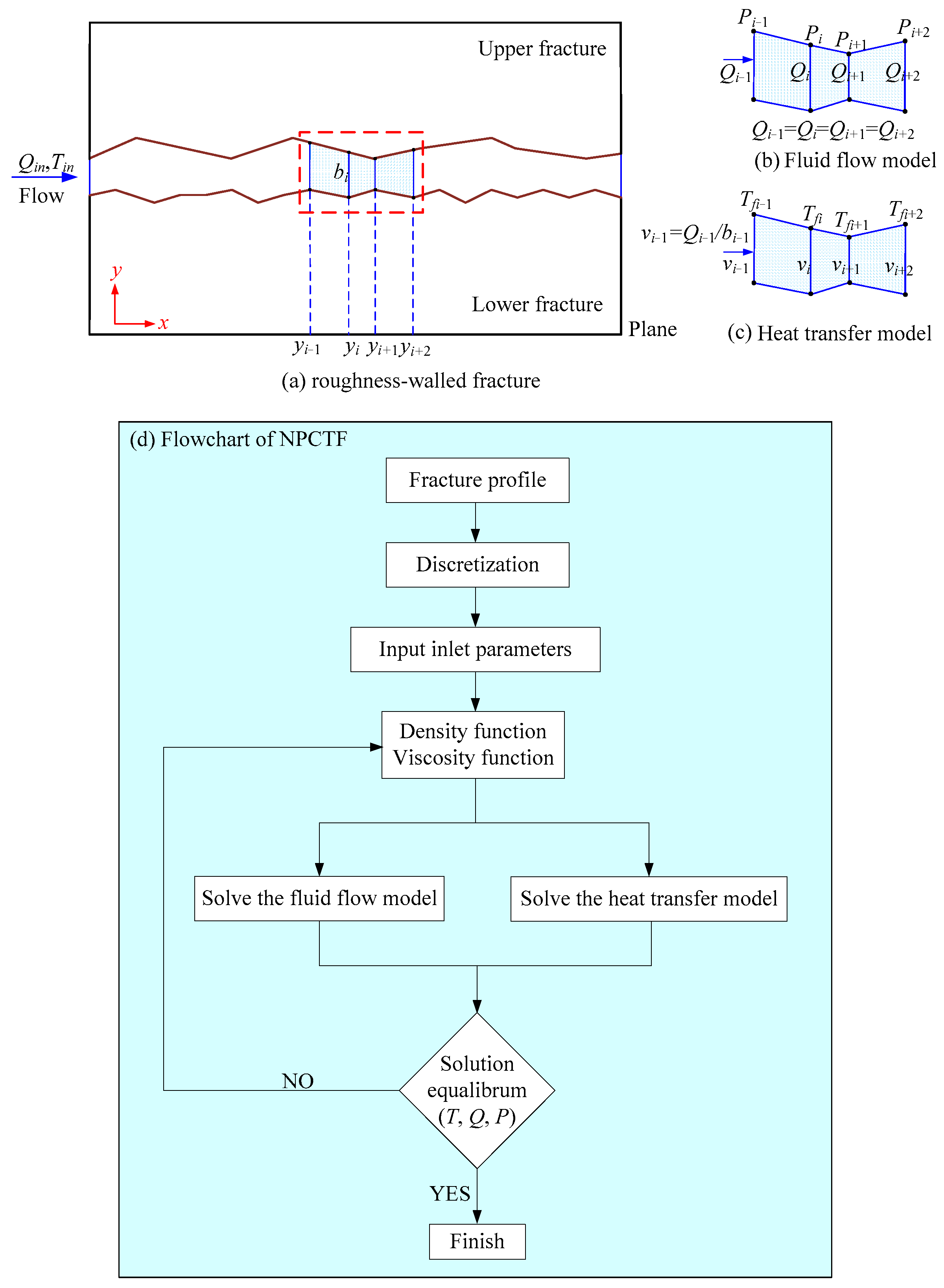
2. Fluid Flow Model
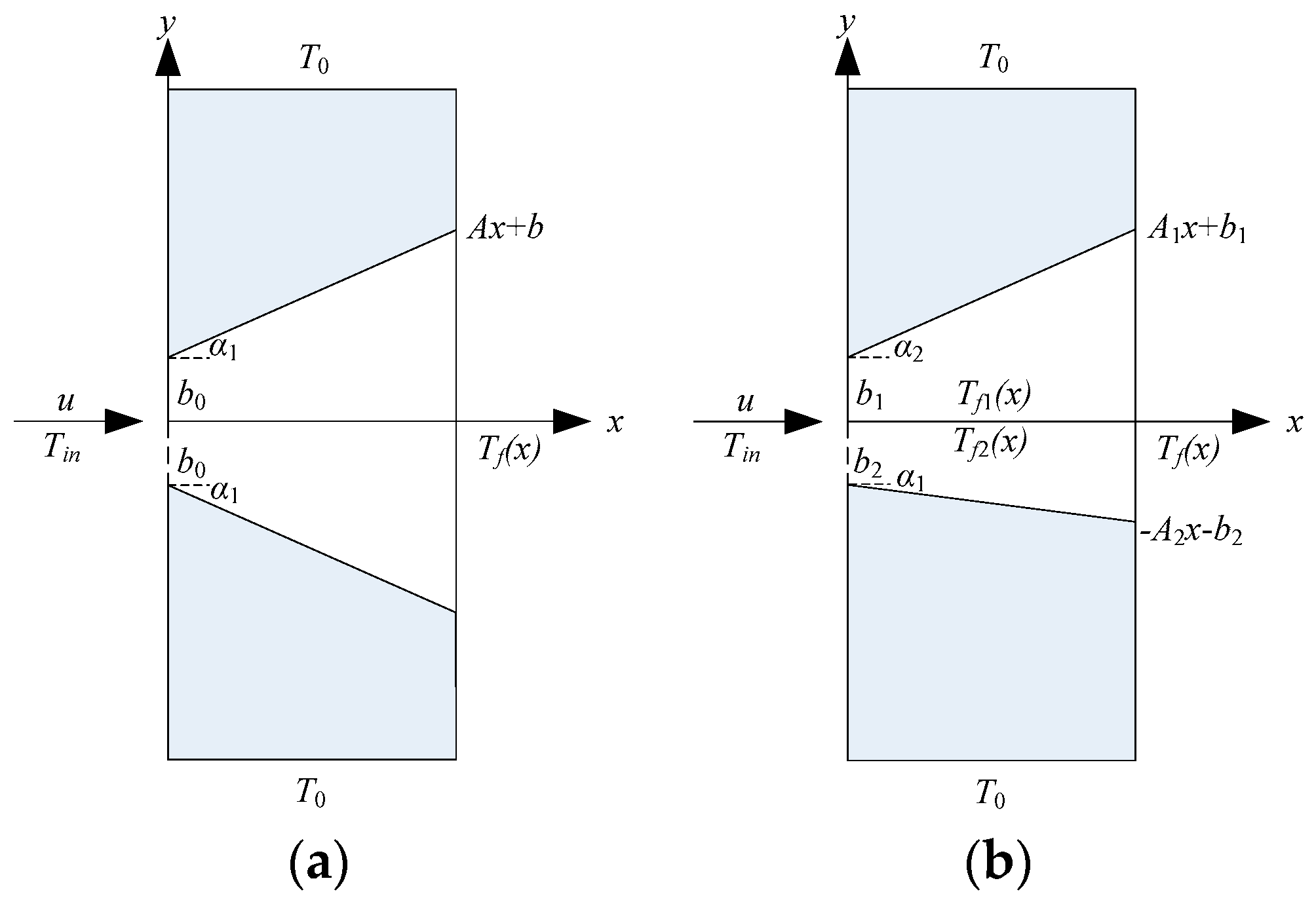
3. Heat Transport Model
- (1)
- Symmetric fracture wedge
- (2)
- Asymmetric fracture wedge
4. Procedure for Coupled Simulation of Thermal and Fluid Flow Models (NPCTF)
4.1. Model Description
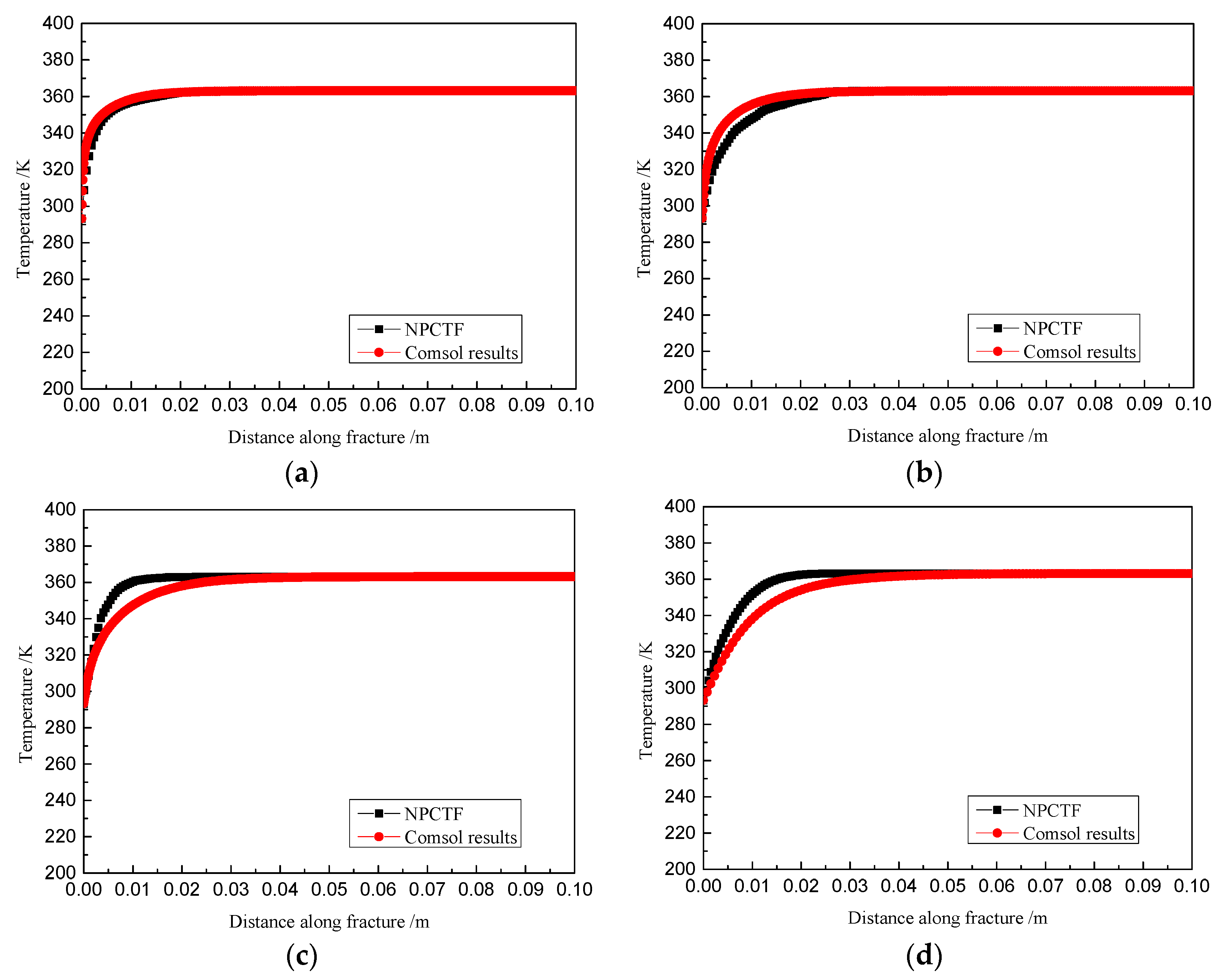
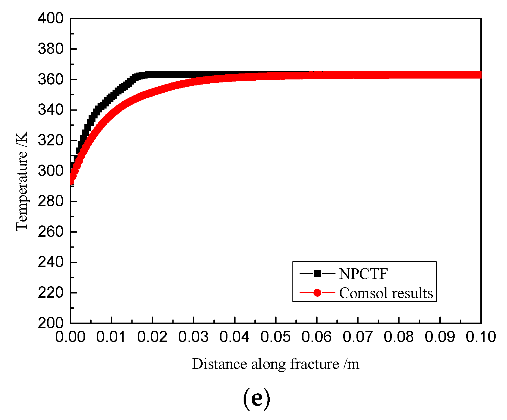
4.2. Validation of NPCTF
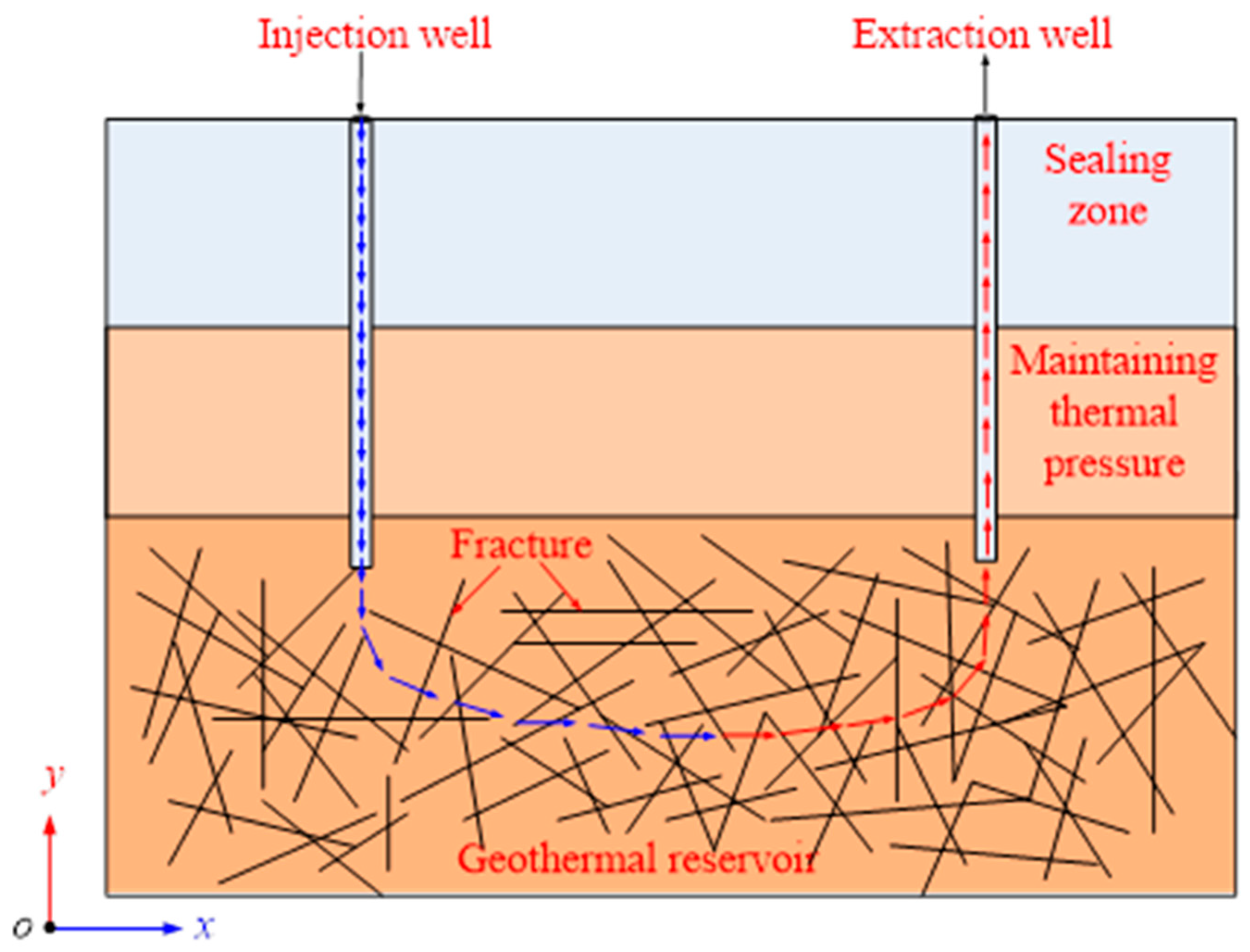
5. Coupled Hydrothermal Simulation in Three-Dimensional Rock Fracture
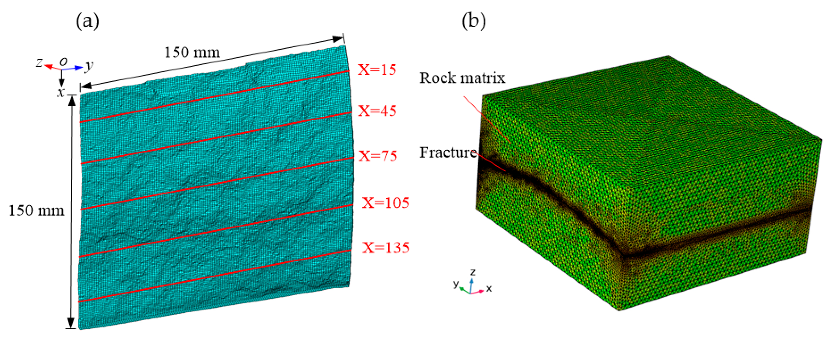
5.1. Modelling Setup
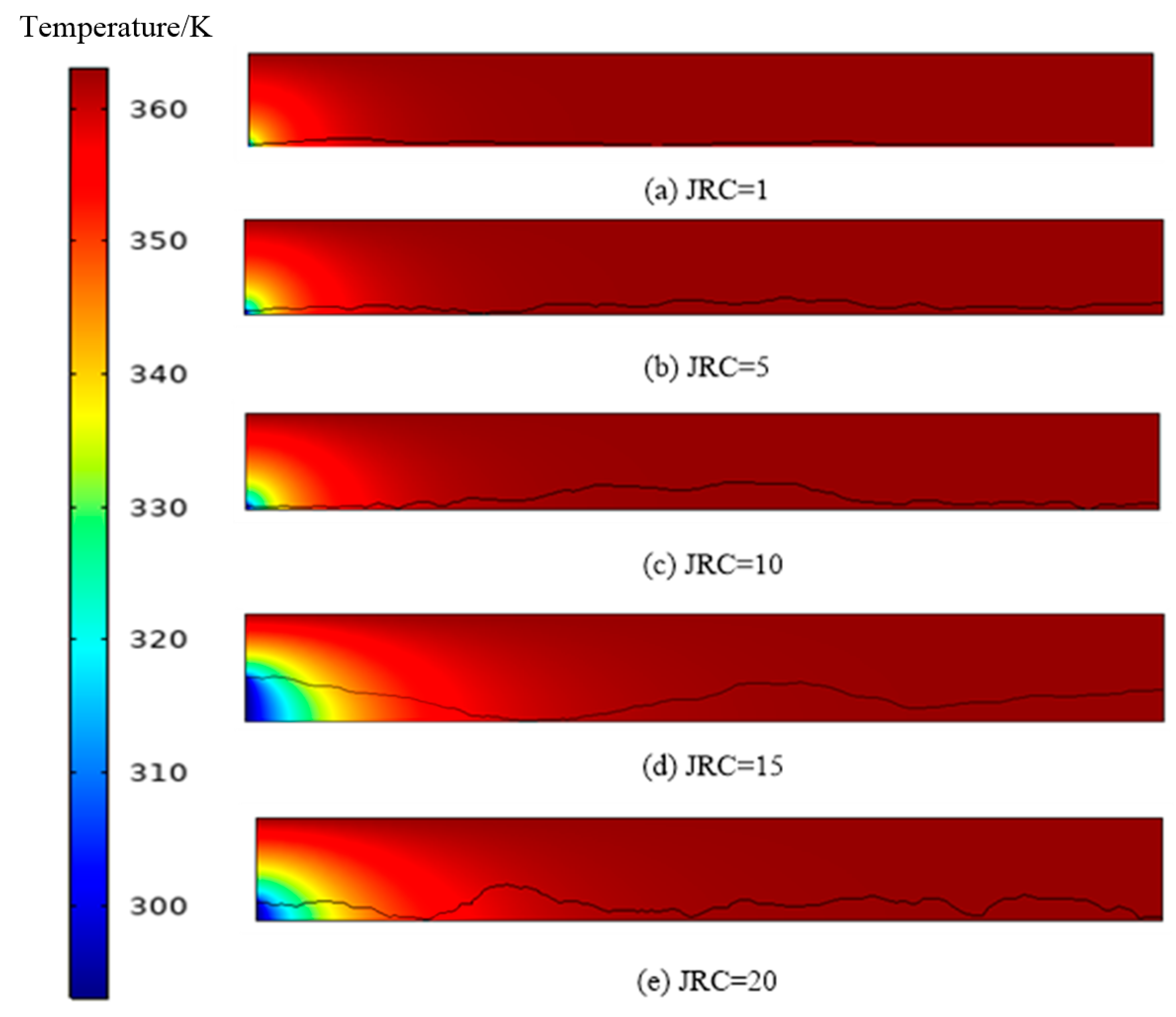
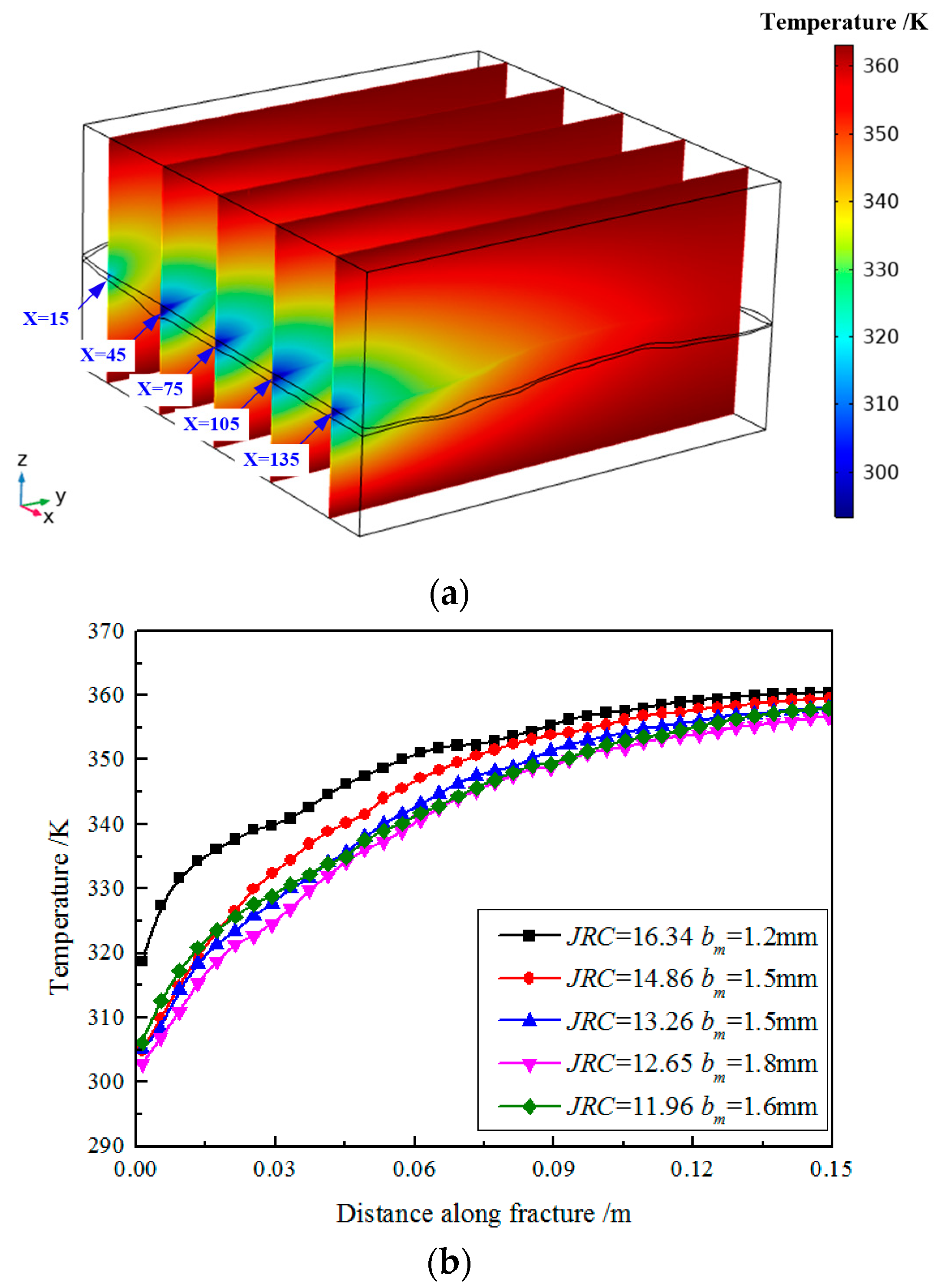
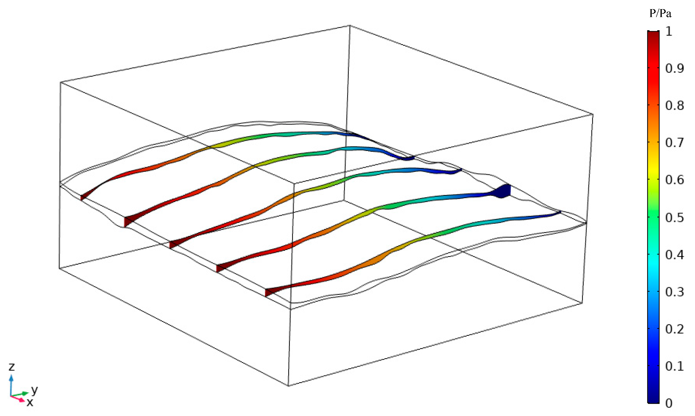
5.2. Temperature and Pressure Distribution Along Fracture
6. Model Performance
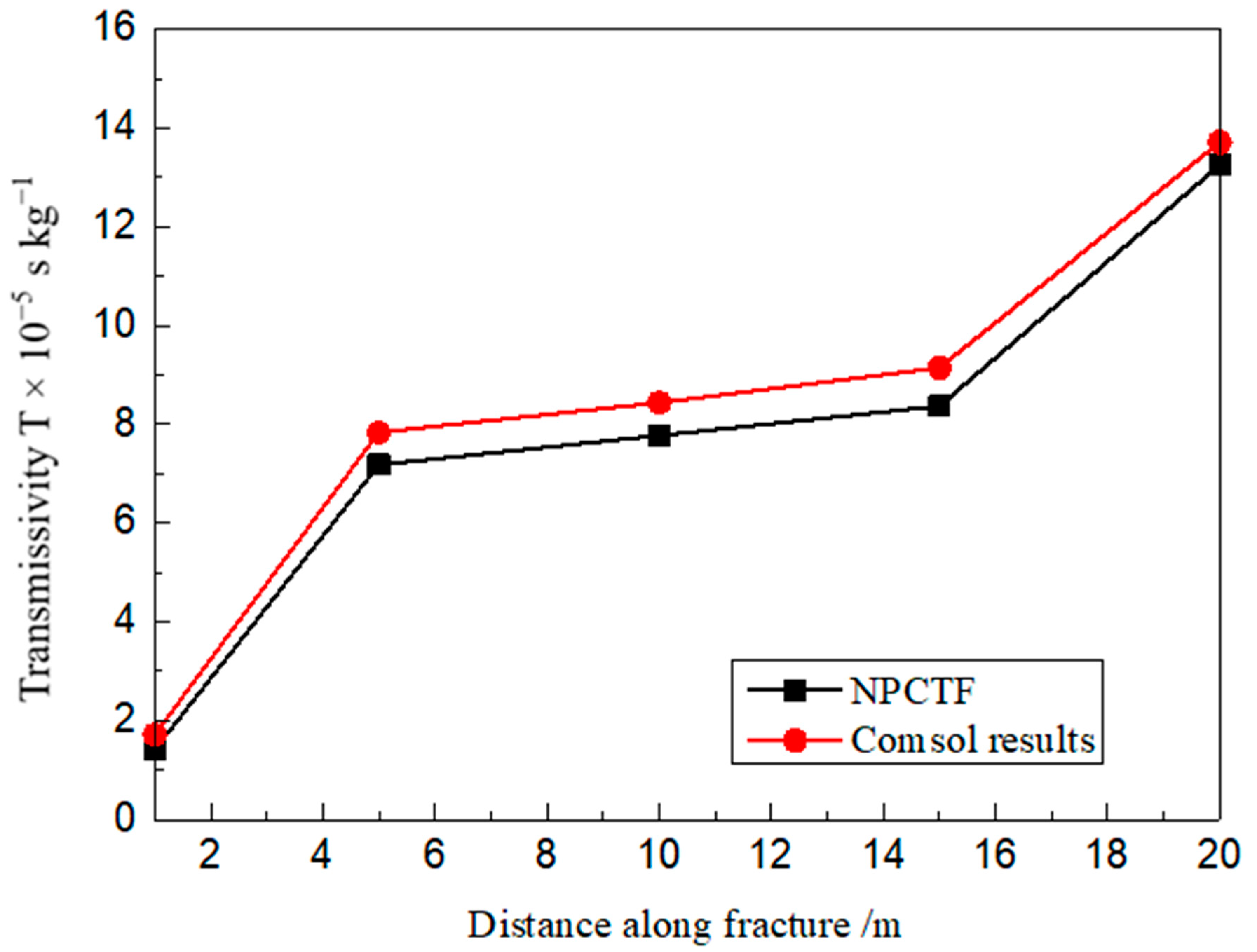
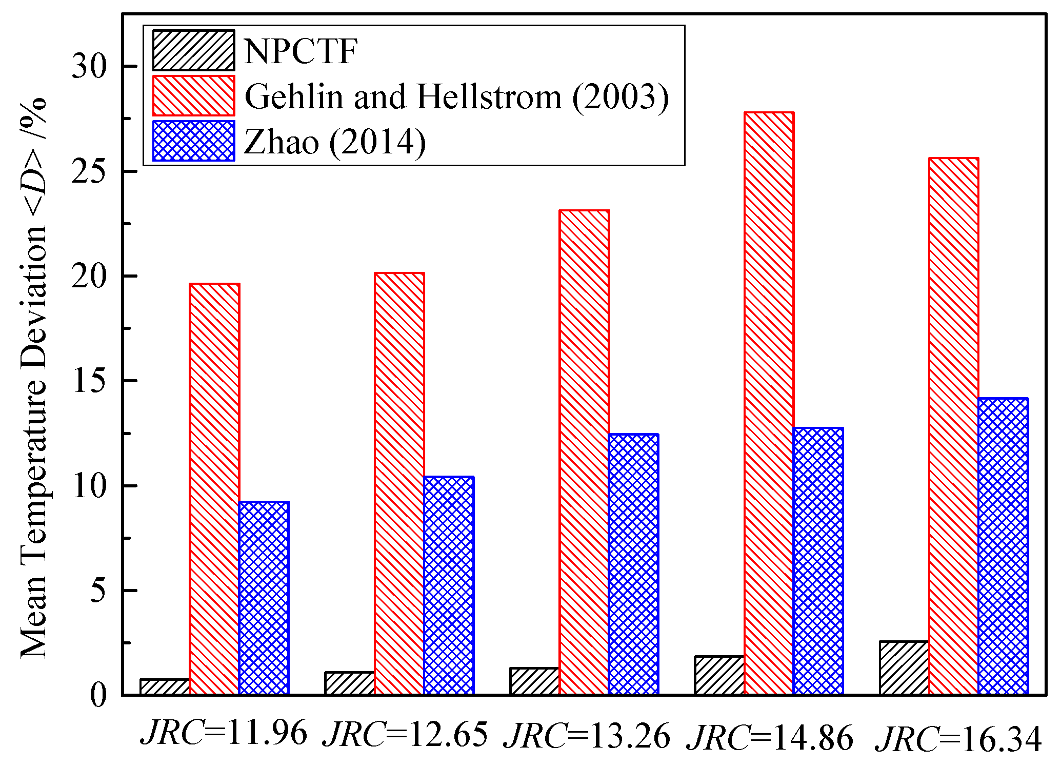
6.1. Comparison with Previous Models from the Literature
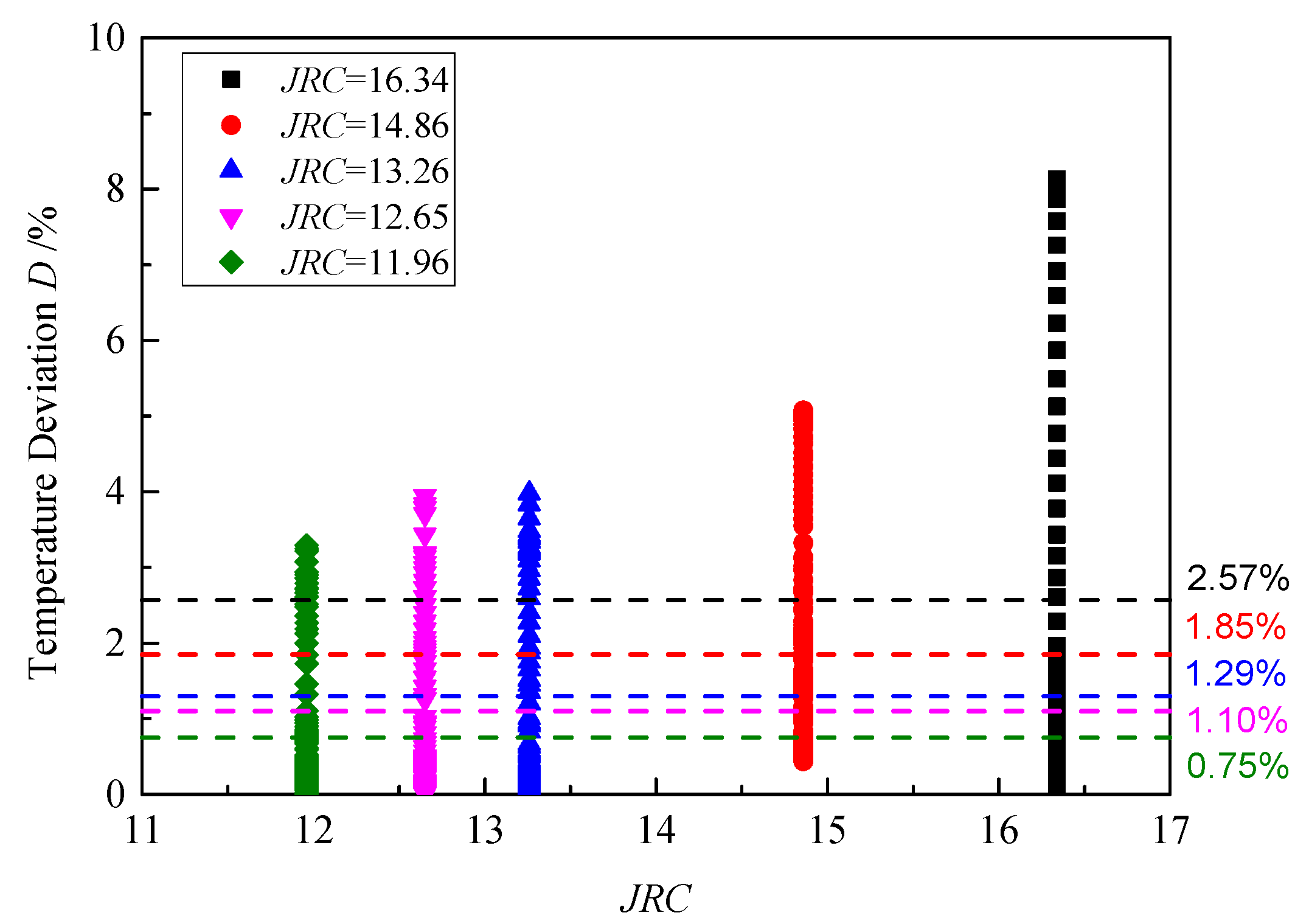
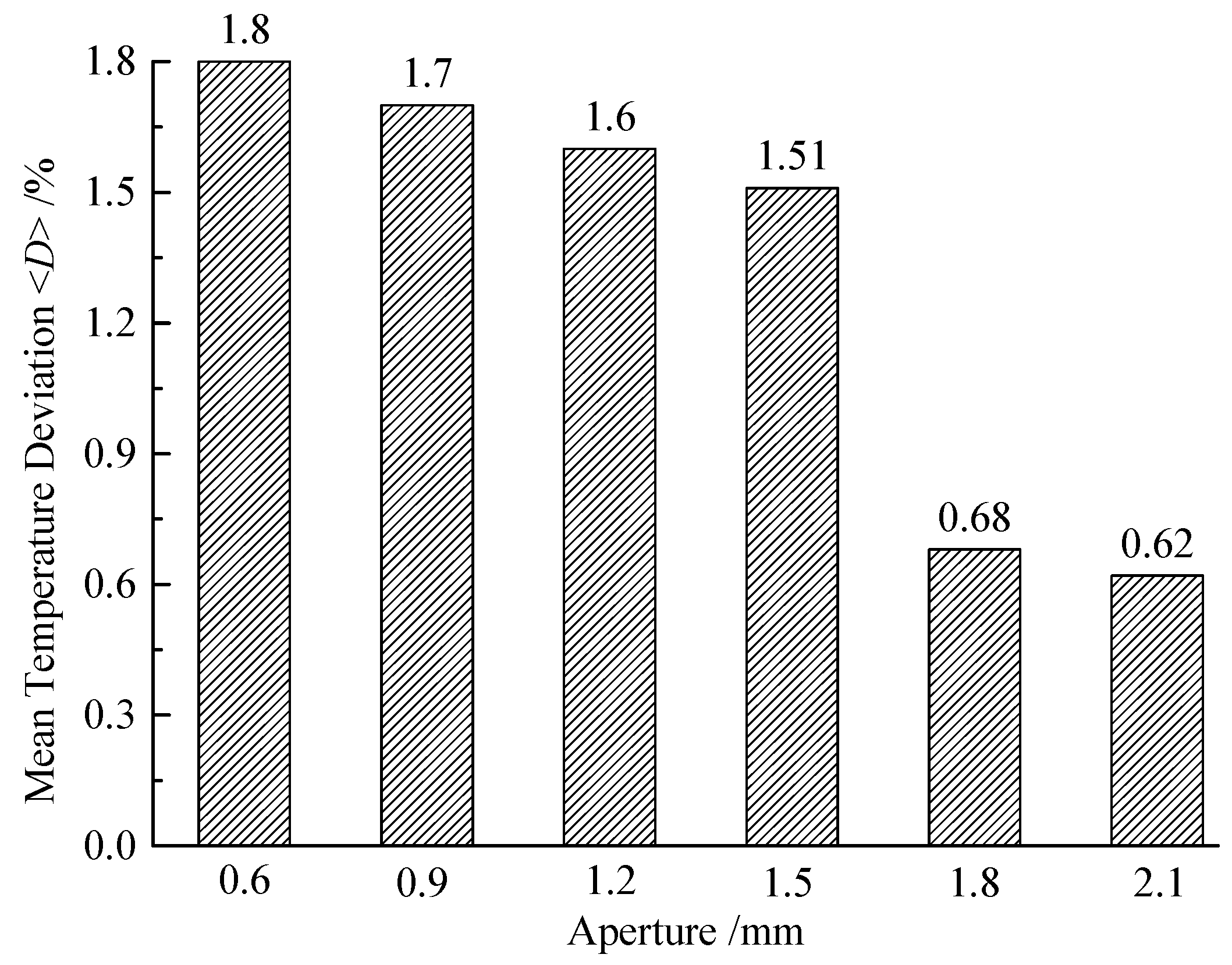
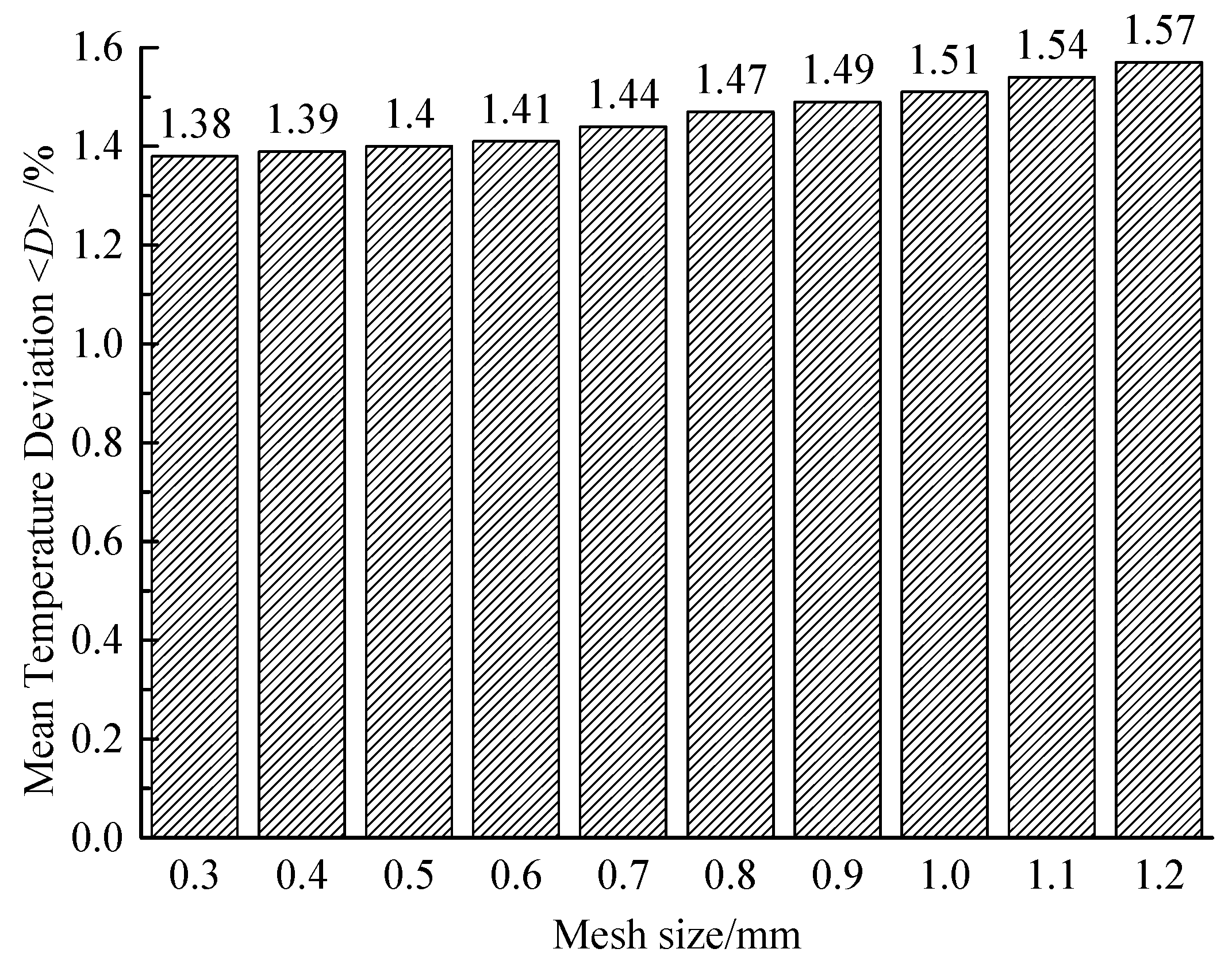
6.2. Sensitivity Analysis
6.3. Limitations of NPCTF
7. Conclusions
Author Contributions
Funding
Institutional Review Board Statement
Informed Consent Statement
Data Availability Statement
Acknowledgments
Conflicts of Interest
Abbreviations
| ε | Perturbation parameter |
| X | Dimensionless roughness |
| ω | Dimensionless absolute aperture variation |
| a | Difference between the upper and lower wedge edge |
| B | Dimensionless aperture |
| c | Fracture local aperture |
| cm | Mean aperture |
| B′ | First derivatives of B with respect to X |
| R | Reynolds number |
| Q | Flow rate per unit width of fracture |
| μ | Fluid viscosity |
| ∆P | Dimensionless pressure difference |
| ∆pm | Pressure difference of flow through a fracture with a uniform aperture defined from the cubic law |
| ρw | fluid density |
| cw | Specific heat of fluid; |
| Kw | Fluid thermal conductivity |
| Kr | Rock thermal conductivity |
| v | Steady flow velocity |
| b | Half aperture of the fracture |
| Tf | Bulk temperature of fluid |
| Tr | Temperature of reservoir rock matrix |
| To | rock temperature |
| Tin | water temperature in inlet of fracture |
| R | Height of rock |
| α | Inclined angle |
| δw | Function of P and Tf |
| Ta | transmissivity |
| JRC | Joint roughness coefficient |
| Z2 | root mean square of first derivative of profile |
| D | Relative deviation between two variables |
| <D> | Mean deviation |
References
- Kolditz, O.; Clauser, C. Numerical simulation of flow and heat transfer in fractured crystalline rocks: Application to the hot dry rock site in Rosemanowes (UK). Geothermics 1997, 27, 1–23. [Google Scholar] [CrossRef]
- Gehlin, S.; Hellstrom, G. Influence on thermal response test by groundwater flow in vertical fractures in hard rock. Renew. Energy 2003, 28, 2221–2238. [Google Scholar] [CrossRef]
- Zhao, Y.; Feng, Z.; Feng, Z.; Yang, D.; Liang, W. THM (Thermo-hydro-mechanical) coupled mathematical model of fractured media and numerical simulation of a 3D enhanced geothermal system at 573 K and buried depth 6000-7000 M. Energy 2015, 82, 193–205. [Google Scholar] [CrossRef]
- Jiao, Y.Y.; Zhang, X.L.; Zhang, H.Q.; Li, H.B.; Yang, S.Q.; Li, J.C. A coupled thermo-mechanical discontinuum model for simulating rock cracking induced by temperature stresses. Comput. Geotech. 2015, 67, 142–149. [Google Scholar] [CrossRef]
- Sun, Z.; Zhang, X.; Yao, J.; Wang, H.; Lv, S.; Sun, Z.; Huang, Y.; Cai, M.; Huang, X. Numerical simulation of the heat extraction in EGS with thermal-hydraulic-mechanical coupling method based on discrete fractures model. Energy 2017, 120, 20–33. [Google Scholar] [CrossRef]
- Yao, J.; Zhang, X.; Sun, Z.; Huang, Z.; Liu, J.; Li, Y.; Xin, Y.; Yan, X.; Liu, W. Numerical simulation of the heat extraction in 3D-EGS with thermal-hydraulic-mechanical coupling method based on discrete fractures model. Geothermics 2018, 74, 19–34. [Google Scholar] [CrossRef]
- Yan, C.; Jiao, Y.Y. FDEM-TH3D: A three-dimensional coupled hydrothermal model for fractured rock. Int. J. Numer. Anal. Methods Geomech. 2019, 43, 415–440. [Google Scholar] [CrossRef]
- Ehyaei, M.; Ahmadi, A.; Rosen, M.A.; Davarpanah, A. Thermodynamic Optimization of a Geothermal Power Plant with a Genetic Algorithm in Two Stages. Processes 2020, 8, 1277. [Google Scholar] [CrossRef]
- Davarpanah, A.; Shirmohammadi, R.; Mirshekari, B.; Aslani, A. Analysis of hydraulic fracturing techniques: Hybrid fuzzy approaches. Arab. J. Geosci. 2019, 12, 402. [Google Scholar] [CrossRef]
- Sun, S.; Zhou, M.; Lu, W.; Davarpanah, A. Application of Symmetry Law in Numerical Modeling of Hydraulic Fracturing by Finite Element Method. Symmetry 2020, 12, 1122. [Google Scholar] [CrossRef]
- Zhu, M.; Yu, L.; Zhang, X.; Davarpanah, A. Application of Implicit Pressure-Explicit Saturation Method to Predict Filtrated Mud Saturation Impact on the Hydrocarbon Reservoirs Formation Damage. Mathematics 2020, 8, 1057. [Google Scholar] [CrossRef]
- Hu, X.; Xie, J.; Cai, W.; Wang, R.; Davarpanah, A. Thermodynamic effects of cycling carbon dioxide injectivity in shale reservoirs. J. Pet. Sci. Eng. 2020, 195, 107717. [Google Scholar] [CrossRef]
- Xiong, F.; Jiang, Q.; Xu, C. Fast Equivalent Micro-Scale Pipe Network Representation of Rock Fractures Obtained by Computed Tomography for Fluid Flow Simulations. Rock Mech. Rock Eng. 2020, 1–17. [Google Scholar] [CrossRef]
- Xiong, F.; Wei, W.; Xu, C.; Jiang, Q. Experimental and numerical investigation on nonlinear flow behaviour through three dimensional fracture intersections and fracture networks. Comput. Geotech. 2020, 121, 103446. [Google Scholar] [CrossRef]
- Heimlich, C.; Gourmelen, N.; Masson, F.; Schmittbuhl, J.; Kim, S.W.; Azzola, J. Uplift around the geothermal power plant of Landau (Germany) as observed by InSAR monitoring. Geotherm. Energy 2015, 3, 2. [Google Scholar] [CrossRef]
- Tenzer, H.; Park, C.-H.; Kolditz, O.; McDermott, C.I. Application of the geomechanical facies approach and comparison of exploration and evaluation methods used at Soultz-sous-Forêts (France) and Spa Urach (Germany) geothermal sites. Environ. Earth Sci. 2010, 61, 853–880. [Google Scholar] [CrossRef]
- Xu, C.; Dowd, P.; Tian, Z. A simplified coupled hydro-thermal model for enhanced geothermal systems. Appl. Energy 2015, 140, 135–145. [Google Scholar] [CrossRef]
- Kolditz, O. Modelling flow and heat transfer in fractured rocks: Conceptual model of a 3-D deterministic fracture network. Geothermics 1995, 24, 451–470. [Google Scholar] [CrossRef]
- Natarajan, N.; Xu, C.; Dowd, P.A.; Hand, M. Numerical modelling of thermal transport and quartz precipitation/dissolution in a coupled fracture–skin–matrix system. Int. J. Heat Mass Transf. 2014, 78, 302–310. [Google Scholar] [CrossRef][Green Version]
- Bai, B.; He, Y.; Li, X.; Hu, S.; Huang, X.; Li, J.; Zhu, J. Local heat transfer characteristics of water flowing through a single fracture within a cylindrical granite specimen. Environ. Earth Sci. 2016, 75, 1460. [Google Scholar] [CrossRef]
- Li, Z.; Feng, X.; Zhang, Y.; Zhang, C.; Xu, T.; Wang, Y. Experimental research on the convection heat transfer characteristics of distilled water in manmade smooth and rough rock fractures. Energy 2017, 133, 206–218. [Google Scholar] [CrossRef]
- Tsang, Y. The effect of tortuosity on fluid flow through a single fracture. Water Resour. Res. 1984, 20, 1209–1215. [Google Scholar] [CrossRef]
- Brown, S. Fluid flow through rock Joints-the effect of surface roughness. J. Geophys. Res. 1987, 92, 1337–1347. [Google Scholar] [CrossRef]
- Xiong, F.; Jiang, Q.; Ye, Z.; Zhang, X. Nonlinear flow behavior through rough-walled rock fractures: The effect of contact area. Comput. Geotech. 2018, 102, 179–195. [Google Scholar] [CrossRef]
- Zou, L.; Jing, L.; Cvetkovic, V. Roughness decomposition and nonlinear fluid flow in a single rock fracture. Int. J. Rock Mech. Min. Sci. 2015, 75, 102–118. [Google Scholar] [CrossRef]
- Wang, M.; Chen, Y.; Ma, G.; Zhou, J.; Zhou, C. Influence of surface roughness on nonlinear flow behaviors in 3D self-affine rough fractures: Lattice Boltzmann simulations. Adv. Water Resour. 2016, 96, 373–388. [Google Scholar] [CrossRef]
- Yin, Q.; Ma, G.; Jing, H.; Wang, H.; Su, H.; Wang, Y.; Liu, R.C. Hydraulic properties of 3D rough-walled fractures during shearing: An experimental study. J. Hydrol. 2017, 55, 169–184. [Google Scholar] [CrossRef]
- He, Y.; Bai, B.; Hu, S.; Li, X. Effects of surface roughness on the heat transfer characteristics of water flow through a single granite fracture. Comput. Geotech. 2016, 80, 312–321. [Google Scholar] [CrossRef]
- Huang, Y.; Zhang, Y.; Yu, Z.; Ma, Y.; Zhang, C. Experimental investigation of seepage and heat transfer in rough fractures for enhanced geothermal systems. Renew. Energy 2019, 135, 846–855. [Google Scholar] [CrossRef]
- Ma, Y.; Zhang, Y.; Yu, Z.; Huang, Y.; Zhang, C. Heat transfer by water flowing through rough fractures and distribution of local heat transfer coefficient along the flow direction. Int. J. Heat Mass 2018, 119, 139–147. [Google Scholar] [CrossRef]
- Gringarten, A.C.; Witherspoon, P.A.; Ohnishi, Y. Theory of heat extraction from fractured hot dry rock. J. Geophys. Res. 1975, 80, 1120–1124. [Google Scholar] [CrossRef]
- Cheng, A.; Ghassemi, A.; Detournay, E. Integral equation solution of heat extraction from a fracture in hot dry rock. Int. J. Numer. Anal. Methods Geomech. 2001, 25, 1327–1338. [Google Scholar] [CrossRef]
- Martínez, A.R.; Roubinet, D.; Tartakovsky, D.M. Analytical models of heat conduction in fractured rocks. J. Geophys. Res. 2014, 119, 83–98. [Google Scholar] [CrossRef]
- Zhao, Z. On the heat transfer coefficient between rock fracture walls and flowing fluid. Comput. Geotech. 2014, 59, 105–111. [Google Scholar] [CrossRef]
- Yost, K.; Valentin, A.; Einstein, H. Estimating cost and time of wellbore drilling for Engineered Geothermal Systems (EGS)–Considering uncertainties. Geothermics 2015, 53, 85–99. [Google Scholar] [CrossRef]
- Brush, D.J.; Thomson, N.R. Fluid flow in synthetic rough-walled fractures: Navier-Stokes, Stokes, and local cubic law simulations. Water Resour. Res. 2003, 39, 1085. [Google Scholar] [CrossRef]
- Wang, Z.; Xu, C.; Dowd, P. Perturbation Solutions for Flow in a Slowly Varying Fracture and the Estimation of Its Transmissivity. Transp. Porous Media 2019, 128, 97–121. [Google Scholar] [CrossRef]
- Wang, Z.; Xu, C.; Dowd, P.; Xiong, F.; Wang, H. A non-linear version of the Reynolds equation for flow in rock fractures with complex void geometries. Water Resour. Res. 2020, 56, e2019WR026149. [Google Scholar] [CrossRef]
- Zimmerman, R.; Al-Yaarubi, A.; Pain, C.; Grattoni, C. Non-linear regimes of fluid flow in rock fractures. Int. J. Rock Mech. Min. Sci. 2004, 41, 163–169. [Google Scholar] [CrossRef]
- Chen, Y.F.; Zhou, J.Q.; Hu, S.H.; Hu, R.; Zhou, C.B. Evaluation of Forchheimer equation coefficients for non-Darcy flow in deformable rough-walled fractures. J. Hydrol. 2015, 529, 993–1006. [Google Scholar] [CrossRef]
- Barton, N.; Bandis, S.; Bakhtar, K. Strength, deformation and conductivity coupling of rock joints. Int. J. Rock Mech. Min. Sci. Geomech. Abstr. 1985, 22, 121–140. [Google Scholar] [CrossRef]
- Tatone, B.; Grasselli, G. Quantitative measurements of fracture aperture and directional roughness from rock cores. Rock Mech. Rock Eng. 2012, 45, 619–629. [Google Scholar] [CrossRef]
- Tse, R.; Cruden, D.M. Estimating joint roughness coefficients. Int. J. Min. Sci. Geomech. Abstr. 1979, 16, 303–307. [Google Scholar] [CrossRef]
- Shaik, A.R.; Rahman, S.S.; Tran, N.H.; Tran, T. Numerical simulation of fluid-rock coupling heat transfer in naturally fractured geothermal system. Appl. Therm. Eng. 2011, 31, 1600–1606. [Google Scholar] [CrossRef]
- Sisavath, S.; Al-Yaarubi, A.; Pain, C.C.; Zimmerman, R.W. A Simple Model for Deviations from the Cubic Law for a Fracture Undergoing Dilation or Closure. Pure Appl. Geophys. 2003, 160, 1009–1022. [Google Scholar] [CrossRef]


| Parameters | Kr/W m−1 K−1 | ρw/kg m−3 | μ/pa s | cw/J kg−1 K−1 | Tin/K | T0/K |
|---|---|---|---|---|---|---|
| Value | 3.5 | 1000 | 0.001 | 4200 | 293.15 | 363.15 |
| Fracture Position | JRC | Mean Aperture/mm |
|---|---|---|
| X = 15 | 14.86 | 1.2 |
| X = 45 | 16.34 | 1.5 |
| X = 75 | 13.26 | 1.5 |
| X = 105 | 12.26 | 1.8 |
| X = 135 | 11.96 | 1.6 |
Publisher’s Note: MDPI stays neutral with regard to jurisdictional claims in published maps and institutional affiliations. |
© 2021 by the authors. Licensee MDPI, Basel, Switzerland. This article is an open access article distributed under the terms and conditions of the Creative Commons Attribution (CC BY) license (http://creativecommons.org/licenses/by/4.0/).
Share and Cite
Xiong, F.; Zhu, C.; Jiang, Q. A Novel Procedure for Coupled Simulation of Thermal and Fluid Flow Models for Rough-Walled Rock Fractures. Energies 2021, 14, 951. https://doi.org/10.3390/en14040951
Xiong F, Zhu C, Jiang Q. A Novel Procedure for Coupled Simulation of Thermal and Fluid Flow Models for Rough-Walled Rock Fractures. Energies. 2021; 14(4):951. https://doi.org/10.3390/en14040951
Chicago/Turabian StyleXiong, Feng, Chu Zhu, and Qinghui Jiang. 2021. "A Novel Procedure for Coupled Simulation of Thermal and Fluid Flow Models for Rough-Walled Rock Fractures" Energies 14, no. 4: 951. https://doi.org/10.3390/en14040951
APA StyleXiong, F., Zhu, C., & Jiang, Q. (2021). A Novel Procedure for Coupled Simulation of Thermal and Fluid Flow Models for Rough-Walled Rock Fractures. Energies, 14(4), 951. https://doi.org/10.3390/en14040951