A Fault Diagnosis Method for Rolling Bearings Based on Parameter Transfer Learning under Imbalance Data Sets

Abstract

Fault diagnosis under the condition of data sets or samples with only a few fault labels has become a hot spot in the field of machinery fault diagnosis. To solve this problem, a fault diagnosis method based on deep transfer learning is proposed. Firstly, the discriminator of the generative adversarial network (GAN) is improved by enhancing its sparsity, and then adopts the adversarial mechanism to continuously optimize the recognition ability of the discriminator; finally, the parameter transfer learning (PTL) method is applied to transfer the trained discriminator to target domain to solve the fault diagnosis problem with only a small number of label samples. Experimental results show that this method has good fault diagnosis performance.

1. Introduction

Fault diagnosis is the core of machinery health management. The purpose of fault diagnosis is to monitor the operation status of equipment or mechanical system, mine the fault feature information according to the operation status, and then diagnose the feature information before the machinery fails to stop [1]. Rolling bearings are a key component of rotating machinery, which is widely used in gearbox, engines, gas turbines, and other machines. The fault diagnosis of rolling bearings is closely related to the safe operation of rotating machinery. However, in practical application, the fault data of rolling bearings is often difficult to obtain, as when the new equipment is often in normal operation, there are few failures in a short time, thus normal data are easy to collect, while fault data such as fault location, generation mode, and damage degree are difficult to collect [2]. Secondly, it is necessary to label and sort the collected fault data, but this is a huge workload, time-consuming, and requires a lot of manpower, material, and financial resources. Therefore, even if a large amount of data for analysis is obtained, the computing equipment must have strong computing capabilities for storage and calculation. To sum up, in actual industrial production, it is very time-consuming and expensive to collect enough label data [3], sometimes even impossible. Therefore, it is of great practical significance to study the new method of rolling bearings fault diagnosis under the imbalance samples.

Transfer learning [4] is a popular method to solve the problem of unbalanced datasets. According to its features, target domain, and learning method, transfer learning can be divided into sample-based transfer learning, feature-based transfer learning, parameter-based transfer learning, and relationship-based transfer learning [5]. The sample-based transfer learning method performs transfer learning by reusing data samples according to certain weight generation rules [6]. The principle of this method is easy to understand, and the operation process is simple and easy to implement. Its limitation lies in that it is only applicable to the case where the data in the source domain and target domain have little difference or obey the same distribution. The feature-based transfer learning method is to select the common features in the source domain and target domain through machine learning and then use the feature transformation method to build the model so as to achieve the ideal transfer effect. However, if the feature selection and transformation method are not reasonable, it is easy to overfit. At the same time, the optimization process usually requires high computational cost [7]. The necessary condition of the parameter-based transfer learning method is to make it clear that the data in the source domain and the target domain can share model parameters. Usually, fine-tuning in the neural network can be used to better adapt to the new task field; this method has generalization and universality [8]. Relationship-based transfer learning performs analogical transfer by mining, analyzing, and learning the logical relationship between data. This method is only suitable for the scenario with a small difference and high similarity between the source domain and target domain. If the difference between the source domain and the target domain is large and the similarity is low, it is difficult to obtain the logical relationship and the transfer effect will be affected [9].

Although transfer learning has achieved promising results in fault diagnosis of machinery, the methods commonly have the following shortcomings: first, most of these them still need a certain amount of labeled data, for example, reference [10,11] require more than 10 target training samples to achieve effective recognition accuracy; Second, we need to do a lot of preprocessing work, such as to extract features [12] from spectrum data rather than the original vibration data; and finally, these methods only transfer the simulation experiment data set to another simulation experiment data set [13], and the speed, loading, and fault degree of these data sets changed slightly, so the generalization ability of these methods are limited. To deal with the above-mentioned limitations, a new deep transfer learning network, named the transferred discriminator network (TD), is proposed for fault diagnose of rolling bearings in this paper. The main contributions of this paper are summarized as follows:

A constrains term was introduced into the sparse auto encoder. The introduction of constrains not only effectively extracts the features of sensor data, but also greatly reduces the size of the sparse auto encoder network.

The constrained sparse auto encoder units were constructed to replace the discriminator of the generative adversarial network and adaptively identify the data from the generator. The dynamic data recalibrations make the distribution of the data from the source domain and generated domain tend to be consistent, thus improving the information distinguishability of generative adversarial network.

A new transferred discriminator network is proposed by transferring the parameters of the generative adversarial network based on the constrained sparse auto encoder units. The proposed TD is able to provide accurate fault estimations based on imbalanced data set of rolling bearings and is superior to some existing diagnosis approaches.

The rest of the paper is organized as follows: Section 2 discusses the existing research status. The framework of the proposed method and related technology are drawn in Section 3. The process of model construction and training are introduced in Section 4. In Section 5, we analyze and compare the existing and proposed method. Section 6 concludes this paper.

2. Related Works

At present, the common fault diagnosis methods under the conditions of only a few samples mainly include traditional methods, deep learning, and transfer learning. Traditional fault diagnosis mostly adopts artificial neural network (ANN) and support vector machine (SVM). For example, Liu et al. [14] applied a small amount of labeled data to expand the anomaly detection model based on single-class SVM in a semi-supervised manner, and employed active learning to reduce the cost of manual labeling. Li et al. [15] constructed a class scale shift-oriented model of a support vector machine when unlabeled data accounted for a small proportion of the total. However, these methods based on shallow machine learning models need to re-extract features for different tasks, requires sufficient prior knowledge and a lot of time. At the same time, the generalization ability of the manually extracted features is weak, which cannot guarantee the robustness and stability of these methods.

Deep learning methods are designed to automatically capture representative features from raw data, thereby improving the performance of fault recognition. At present, it has been widely used in the field of fault diagnosis. For example, Min et al. [16] proposed an intelligent fault diagnosis method, which uses a deep neural network (DNN) based on stacked noise reduction automatic encoder, and applies this encoder to unlabeled data in an unsupervised way to learn representative features. Wang et al. [17] introduced a recognition method based on deep learning. After transforming the controlled auto regressive (CAR) model into a finite impulse response (FIR) model, a deep auto encoder was adopted to train the model with a small amount of unlabeled data, and this method has higher recognition accuracy than the back propagation (BP) neural network. Obviously, compared with traditional methods, the deep encoder can automatically extract features, but the sparsity of the automatic encoder is not considered in the above methods. The sparser the encoder is, the smaller the reconstruction error is, and the more representative features can be extracted. In order to solve this problem, Chen et al. [18] realized a deep self-coding network with a new L1/L2 norm of the cost function to diagnose the equipment operation status under different security risk levels. The experimental results show that the method can increase the sparsity of the coding network, reduce the reconstruction errors, and extract more representative features. However, the above method must meet two prerequisites at the same time; one is sufficient sample label data, and the other is the training samples and the test samples that are independent and identically distributed, however in practical applications, it is often difficult to meet [19].

Transfer learning is an emerging method by applying the acquired knowledge or model to the relevant domain and improving its learning performance [20]. Because of its ability of generalization, effectiveness, and robustness where there are few label samples, it is widely used in image processing, medical treatment, natural language processing, and other fields and has become a research hotspot in fault diagnosis in recent years. In reference [21], a small number of label samples in the target domain were adopted to supervise the training of sparse automatic encoder, features extracted by the second encoder, and then a support vector machine was used for fault diagnosis. Li et al. [22] designed a method of transferring a deep noise reduction auto encoder in order to effectively solve the problem of fault diagnosis of aircraft key mechanical parts with few label samples. Yang et al. [23] solved the fault diagnosis problem of internal combustion engines under the condition of little labeled data and incomplete fault samples of a single machine by using the transfer learning idea, which greatly improved the effect compared with the traditional method.

3. Framework of the Proposed Method

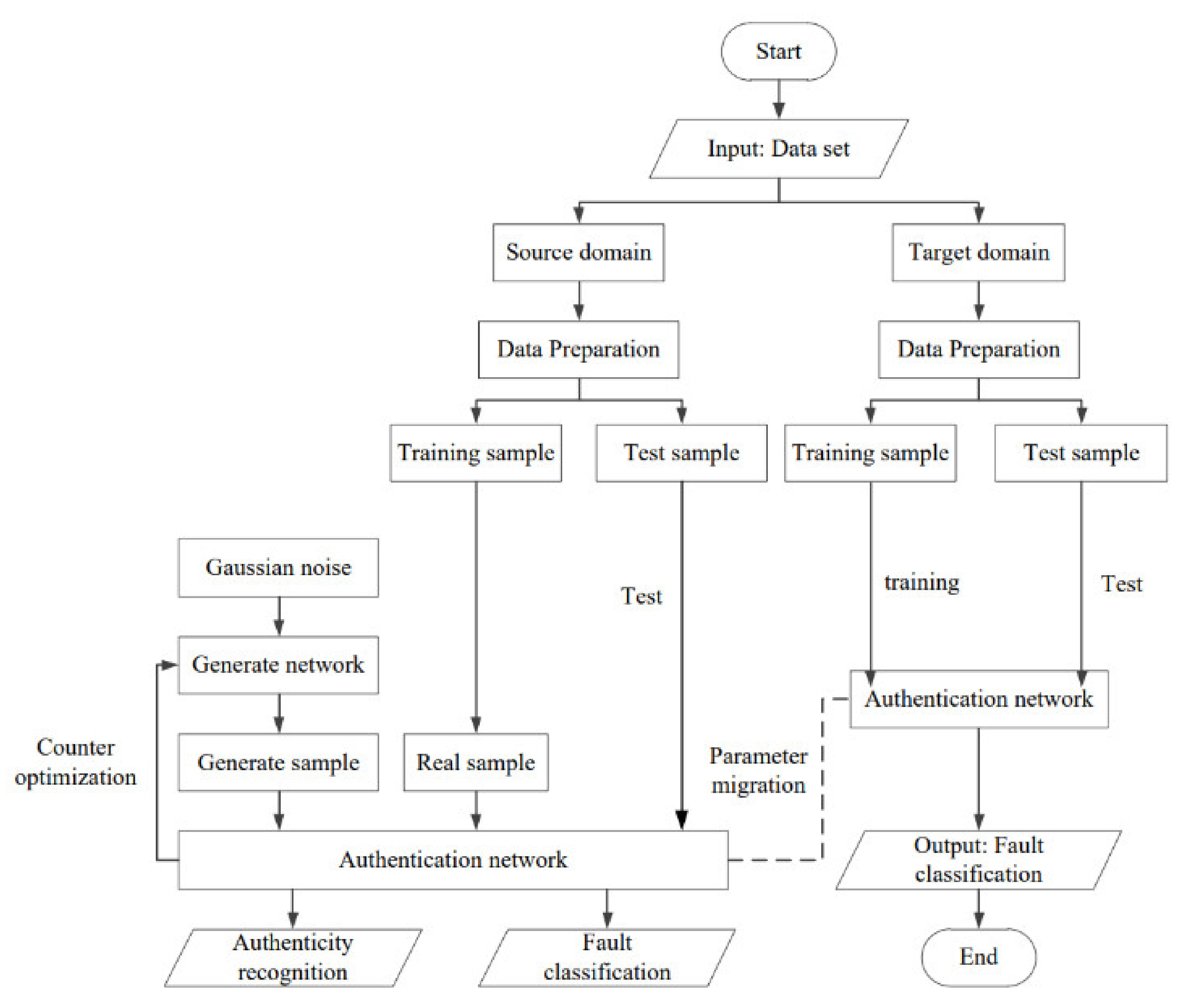
This paper proposes a fault diagnosis model named a transferred discriminator (TD) based on few sample labels. The basic idea is: first add a new constraint to the sparse auto encoder to enhance sparsity; second, stack multiple constrained sparse auto encoders (CSAE) to form a deep constrained sparse auto encoder (DCSAE), and as the discriminator of the generative adversarial network, we call this discriminator DGAN (DCSAE as a discriminator in GAN); then, the classification and recognition ability of DGAN was optimized by using the adversarial mechanism of GAN; finally, the parameters of the discriminator in DGAN were transferred to the target discriminator TD by the parameter transfer method, and the discriminator was fine-tuned with a small amount of labeled data in the target domain, and the fault classification and identification was ultimately realized. The framework of the proposed method is depicted in Figure 1.

Specific steps are as follows:

Step one: data preprocessing. The data set of the source domain and target domain are normalized, as shown in Equation (1).

$$x^{\ast }=\frac{x-x_{\min }}{x_{\max }-x_{\min }}$$

(1)

where $x_{\max }$ is the maximum value of the sample data, and $x_{\min }$ is the minimum value of the sample data.

Step two: DGAN training. First, stack multiple CSAEs to construct a deep network DGAN, and then divide the data $X_s$ of the source domain into a training sample $X_{sd}$ and a test sample $X_{se}$, and use the source domain training data $X_{sd}$ to train DGAN, test the performance of the discriminator by test sample $X_{se}$ to obtain trained DGAN.

Step three: parameter transfer. First, for data $X_t$ of the target domain, a small amount of available labeled data $X_{td}$ is selected as training data, and unlabeled data $X_{te}$ is used as test data. At this time, the target deep model TD with the same discriminator structure in DGAN is constructed. Then, the training parameters (including weight and deviation) of the discriminator in DGAN and softmax classifier are transferred to initialize TD and its softmax classifier.

$$V^l=W^l,u^l=b^l,l=1,2,\dots ,L$$

(2)

where $V^l$ is the weight between layer $l$ and layer $l+1$ in TD, b is the biases of both layers.

Step four: TD training. In order to further improve the performance of the model, it is necessary to fine-tune the model as a whole. The TD was fine-tuned by the training data $X_{td}$ of the target domain, and the performance of TD was tested by the test data $X_{te}$ of the target domain, the loss function of the fine-tuning process is Equation (3). Where, $y$ is the class label of the real sample, $y_f$ is the class label of the generated sample, $K_r$ is the class label of the real sample determined by the classifier, $K_f$ is the class label of the generated sample determined by the classifier, N is the real sample, M is the generated sample, $\alpha$ is the nonnegative constraint penalty, L is the layers of the network, $q_l$ represents the hidden unit number of the final auto encoder, V denotes the weights between the final hidden layer and softmax classifier.

$$E_{TD-DCSAE}=-\frac{M{{\displaystyle \sum }}_{n=1}^N{y}^n\ln K_r^n+N{{\displaystyle \sum }}_{m=1}^M{y}_f^m\ln K_f^m}{NM}+\frac{\alpha }{2}{\displaystyle \sum }_{l=1}^L{\displaystyle \sum }_{i=1}^{q_l}{\displaystyle \sum }_{j=1}^{q_l+1}f\left(V_{ji}\left(l\right)\right)$$

(3)

4. Model Constructions and Training

4.1. Constrained Sparse Auto Encoder (CSAE)

Similar to the auto encoder, the sparse auto encoder (SAE) consists of two parts: an encoder and a decoder. The encoder is composed of an input layer and a hidden layer. It mines the hidden effective information of the input data and extracts features while reducing the data dimension. The decoder is composed of a hidden layer and an output layer. The representative features are reconstructed through decoding, and the input data is reproduced as much as possible and used as the output [24].

When extracting representative features from high-dimensional data, over-fitting usually occurs. In order to make the hidden layer expression more sparse, in other words, when the hidden neuron receives a large amount of data, it can still find important structures in the data, so that SAE can effectively extract the underlying essential features from a large amount of data, this paper adds constraints to the SAE to reduce the influence of weights and minimize the cost function (Equation (3)) in the iterative process. Constraints are obtained through unsupervised learning; the constraints proposed in this paper are shown in Equation (4).

$$\mathrm{Constraint}\mathrm{Factor}\mathrm{Term}=\frac{\alpha }{2}{\displaystyle \sum _{l=1}^2{\displaystyle \sum _{i=1}^{q_l}{\displaystyle \sum _{j=1}^{q_l+1}f}}}\left(W_{ji}(l)\right)$$

(4)

$\alpha$ is constraint penalty coefficient, $W_{ji}(l)$ is the weight between node $i$ in layer $l$ and node $j$ in layer $l+1$, the expression of $f(\ast )$ is:

$$f\left(W_{ji}(l)\right)=\left\{\begin{array}{ll}{\left(W_{ji}(l)\right)}^2,\hfill & W_{ji}(l)⩽0\hfill \\ 0,\hfill & W_{ji}(l)>0\hfill \end{array}\right.$$

(5)

$f\left(\ast \right)$ is a weight decay term to prevent weight overfitting. Our goal is to minimize the Equation (4), reduce the number of non-negative weights of each layer and the overall average reconstruction error. We update the weight and biases using the gradient descent algorithm.

4.2. Deep Constrained Sparse Auto Encoder (DCSAE)

These multiple constrained sparse automatic encoders (CSAE) were stacked to form a deep constrained sparse auto encoder (DCSAE) to extract the samples’ deep features. DCSAE consists of an input layer, an output layer and multiple hidden layers. It uses the softmax classifier as the output layer to identify the fault type of the bearings. As shown in Figure 2, the training of the model is carried out in two stages: (1) unsupervised layer-by-layer greedy initialization stage and (2) supervised fine-tuning stage.

After the depth features of a single CSAE were obtained through layer-by-layer training, the output feature $a=g_s\left(W_{1}X+b_1\right)$ of the previous layer was used as the input data of the next layer, then the output feature of the last hidden layer was adopted as the input to train the softmax classification layer, and its cost function is shown in Equation (6).

$$E_{c-softmax}=-\frac{1}{n}{\displaystyle \sum _{i=1}^n{k}^i}\ln y^i+\frac{\alpha }{2}{\displaystyle \sum _{i=1}^{q_l}{\displaystyle \sum _{j=1}^{C}f}}\left(W_{ji}(l)\right)$$

(6)

where $k$ is the categories identified by softmax, and $C$ is the total categories of bearings failures.

The above is the greedy step-by-step layer training, which lays the foundation for the final fine-tuning. Finally, the overall cost function of DCSAE was constructed. By minimizing the cost function, the network model was fine-tuned to obtain better fault recognition results, as shown in Equation (7).

$$E_{DCSAE}=-\frac{1}{n}{\displaystyle \sum _{i=1}^n{c}^i}\ln y^i+\frac{\alpha }{2}{\displaystyle \sum _{l=1}^L{\displaystyle \sum _{i=1}^{q_l}{\displaystyle \sum _{j=1}^{q_l+1}f}}}\left(W_{ji}(l)\right)$$

(7)

The related description of the DCSAE training algorithm is shown in Algorithm 1.

Algorithm 1 DCSAE Training Algorithm

Input: Learning rate learning_rats, Training batch training_epochs, Training data size batch_size, the number of hidden layer num.

Output: Classification results

1: For $i$ in num:

2: Initialize weight $w_1$, $w_2$, deviation $b_1$, $b_2$

3: For $i$ in num:

4: $laye{r}_i=x\ast w_1(encode{r}_i)+b_1(encode{r}_i)$

5: $g_s(x)=1/(1+\exp (-x))$

6: $laye{r}_i=x\ast w_1(decode{r}_i)+b_1(decode{r}_i)$

7: $encoder\_op=encoder\left(x\right)$ $encoder\_result=encoder\_op$ $decoder\_op=decoder\left(encoder\_op\right)$

8: $MSE=\frac{1}{2n}\left({\displaystyle \sum _{i=1}^n{‖X_{Ri}-X_i‖}^2}\right)$

9: $KL=\beta {\displaystyle \sum _{i=1}^{q_l}\left(r\log \frac{r}{{\widehat{r}}_j}+(1-r)\log \frac{1-r}{1-{\widehat{r}}_j}\right)}$

10: $\mathrm{Constraint}\mathrm{Factor}\mathrm{Term}=\frac{\alpha }{2}{\displaystyle \sum _{l=1}^2{\displaystyle \sum _{i=1}^{q_l}{\displaystyle \sum _{j=1}^{q_l+1}f}}}\left(W_{ji}(l)\right)$

11: $optimizer=Adam\left(learning\_rate\right).\min imize(loss)$

12: $init=tf.global\_variables\_initializer()$

13: $batch=int\left(mnist.train.num\_examples/batch\_size\right)$

14: For epoch in $training\_epochs:$

15: For $i$ in batch:

16: $batch\_xs,batch\_ys=mnist.train.next\_batch\left(batch\_size\right)$

17: $c=sess.run([optimizer,loss],feed\_dict=\{X:batch\_xs\})$

18: End

19: End function

4.3. Model Training

The above-mentioned DCSAE was used as the discriminator of GAN [25] and form DGAN. The generator of DGAN was composed of an input layer, a hidden layer, and an output layer. It learned representative features from high-dimensional data through encoding and decoding to generate more realistic samples. Firstly, the random noise ${\left\{z^m\right\}}_{m=1}^m$ sampled from Gaussian distribution was input into the coding network to learn the potential features of the samples. Then, a new sample ${\left\{X_{\mathrm{f}}^m\right\}}_{m=1}^M$ was generated by decoding the network, and the corresponding class label was generated.

The discriminator of DGAN can distinguish the true sample from the generated sample and identify the fault type. In the training process, the discriminator generates the loss function of the original GAN, and at the same time, produces the fault identification loss and constraint loss. Therefore, the specific definition of the correlation loss function of the discriminator in the training stage is shown in Equations (8)–(11).

$$E_{DCSAE}^{cla}(D)=-\frac{M{\displaystyle \sum _{n=1}^N{y}^n}\ln k_r^n+N{\displaystyle \sum _{m=1}^M{y}_f^m}\ln k_f^m}{NM}$$

(8)

$$E_{DCSAE}^{con}(D)=\frac{\alpha }{2}{\displaystyle \sum _{l=1}^L{\displaystyle \sum _{i=1}^{q_l}{\displaystyle \sum _{j=1}^{q_l+1}f}}}\left(W_{ji}(l)\right)\left\{\begin{array}{ll}{\left(W_{ji}(l)\right)}^2,\hfill & W_{ji}(l)\le 0\hfill \\ 0,\hfill & W_{ji}(l)>0\hfill \end{array}\right.$$

(9)

$$E_{DCSAE}^{ori}(D)=-\frac{M{\displaystyle \sum _{n=1}^N\ln }{Q}_r^n+N{\displaystyle \sum _{m=1}^M\ln }(1-Q_f^m)}{NM}$$

(10)

$$E_{DCSAE}(D)=argmin(E_{DCSAE}^{cla}(D)+E_{DCSAE}^{con}(D))+E_{DCSAE}^{ori}(D))$$

(11)

$E_{DCSAE}(D)$ is the total loss function of discriminator in DGAN, and $E_{DCSAE}^{cla}(D)$, Among them, $E_{DCSAE}^{con}(D)$ and $E_{DCSAE}^{ori}(D)$ represent the loss function of fault classification, constraint loss function and loss function of original GAN respectively. $y$ is the class label of the real sample, $y_f$ is the class label of the generated sample, $k_r$ is the class label of the real sample determined by the classifier, $k_f$ is the class label of the generated sample determined by the classifier, $Q_r$ is the label of real sample, $Q_f$ is the label of generated sample.

The discriminator recognizes the deception of the generator as much as possible, and judges the real sample is 1, and the generated sample is 0; and the generator should deceive the discriminator as much as possible. In continuous optimization, the discriminator should also judge the generated sample as 1. The update training is achieved by minimizing the loss function, as shown in Equations (12)–(14).

$$E_{DCSAE}^{cla}(G)=-\frac{M{\displaystyle \sum _{n=1}^N{y}^n}\ln k_r^n+N{\displaystyle \sum _{m=1}^M{y}_f^m}\ln k_f^m}{NM}$$

(12)

$$E_{DCSAE}^{ori}(G)=-\frac{1}{M}{\displaystyle \sum _{m=1}^M\ln }{Q}_f^m$$

(13)

$$E_{DCSAE}(G)=argmin(E_{DCSAE}^{cla}(G)+E_{DCSAE}^{ori}(G))$$

(14)

Among them, $E_{DCSAE}(G)$ is the loss function of the generator in the DGAN model, $E_{DCSAE}^{cla}(G)$ and $E_{DCSAE}^{ori}(D)$ respectively represent the loss function of the fault classification and the loss function of the original GAN.

The principle of DGAN training is shown in Figure 3. The core of DGAN training is to alternately run the discriminator and generator through the adversarial learning mechanism and to continuously game and optimize. After calculating the gradient value derived from the above loss function, and training the discriminator and generator using the backpropagation algorithm, the independent adaptive learning rate is designed to update and optimize the different parameters of the DGAN model according to the Adam algorithm.

As depicted in Figure 3, the DGAN training process including four stages. The distribution of the real data set is $P_{data}\left(x\right)$, x is the real sample, z is the random noise. In the first stage, the generator has a weak ability to generate “real” samples, and the discriminator does not have strong discrimination ability, the real sample set and the generated sample set have the largest difference in distribution. In the second stage, firstly, the generator is fixed and the discriminator is trained and optimized. Then input the real sample x, and compare the result label of the discriminator with the label of the real sample (i.e., 1). Next, input the generated sample, and compare the obtained identification label with the label of the generated sample (i.e., 0). The gradient descent method is used to maximize the identification accuracy. It can be seen that the identification ability of the discriminator in the second stage has been improved. In the third stage, firstly, the discriminator is fixed and update generator. Then input random noise z to get the generated sample, label it as 1, and send it to the discriminator for identification. Similarly, the gradient descent method is applied to maximize the identification accuracy. It can be seen that the “authenticity” of the sample generated by the generator is increasingly close to the real sample. In the last stage, the two parts are constantly updated and optimized to improve the fault identification ability and sample generation ability separately until the final convergence and complete the training of the DGAN model.

4.4. Parameter Transfer Learning

After the training of DGAN, the paper adopts parameter transfer learning (PTL) to transfer the discriminator parameters from the trained DGAN to the new discriminator named transferred discriminator (TD), in order to solve the fault diagnose problem under few labeled samples in the target domain, which will reduce the training time and improve the efficiency. The specific definitions of PTL are as follows.

Given a labeled source domain,

$$X_s={\left\{x_{si},y_{sj}\right\}}_{j\in [1,C]}^{i\in [1,n1]}$$

(15)

A target domain with few labels,

$$X_t={\left\{x_{ti},y_{tj}\right\}}_{j\in [1,C]}^{i\in [1,n2]}$$

(16)

$x_{si}$, $y_{sj}$ are source domain data and category labels, $x_{ti}$ and $y_{ti}$ are target domain data and category labels, respectively, C is the number of categories, $n1$ and $n2$ are the number of samples of the source domain and target domain, respectively, and the number of samples with label in target domain is far less than that in source domain $N_{ytj}<<N_{ysj}$.

Then, the fault diagnosis process based on parameter transfer learning can be divided into five steps. The first step is to construct DGAN. The training data of the source domain is used for learning, and the pre-trained DGAN is verified by the test data; The second step is to construct TD, which has the same structure as the discriminator in DGAN; The third step is to transfer the parameters of a discriminator in the DGAN to TD; The fourth step is to fine tune TD by using the limited labeled samples in the target domain; Finally, the effectiveness of the transferred model TD is tested using unlabeled data of target domain.

5. Experiment and Result Analysis

5.1. Experimental Data

In order to verify the fault diagnosis performance of the method in this paper, when the rolling bearings fault data contained only a small amount of label, the data sets of two different domains were analyzed. That is, the rolling bearings data of the experimental center of Case Western Reserve University was used as the source domain data set. The rolling bearings data collected from real mechanical equipment was used as the target domain data set. 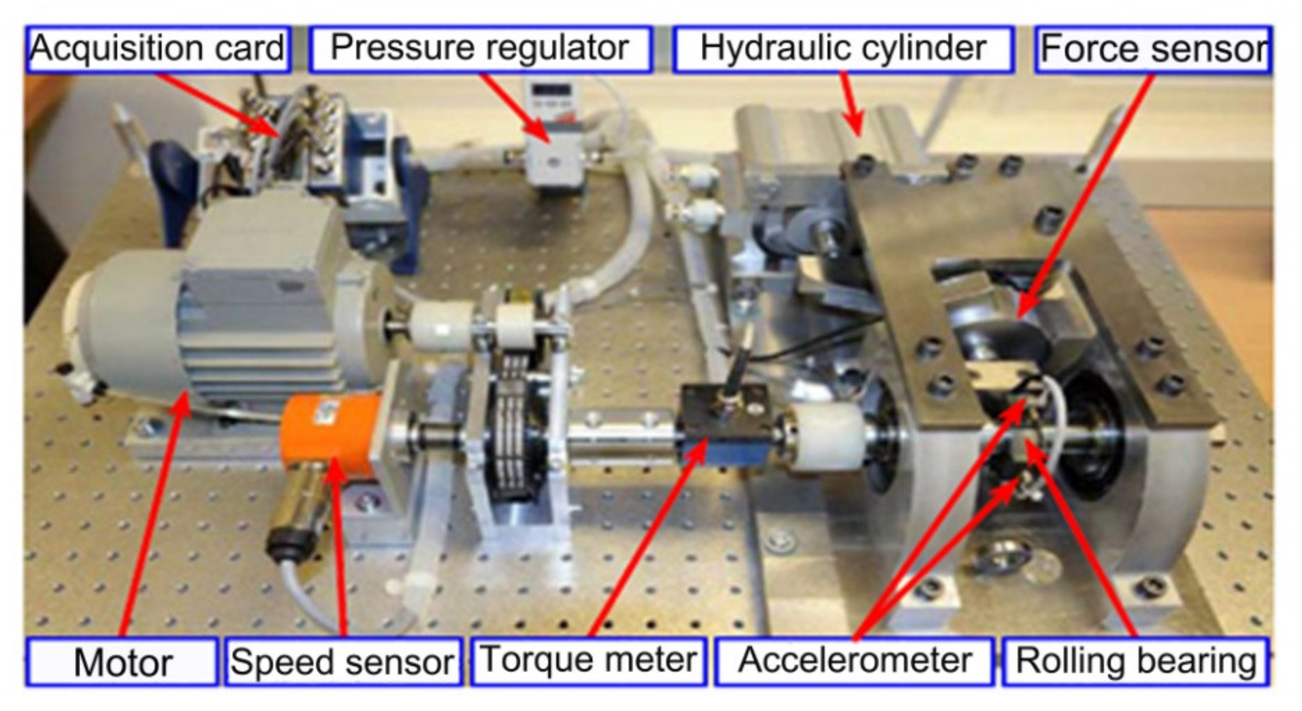Figure 4 is target domain data set acquisition equipment [26]. As shown in Figure 4, two accelerometers were installed on the test bench to measure the horizontal and vertical vibration signals. These accelerometers measured the raw vibration signal at 10 s intervals with a sampling frequency of 10.24 kHz. This means that 1024 data points were available every 10 s.

(1)

Source domain data set

Taking the bearing model SKF6205 as the research object to collect relevant data. In the source domain data set, the single point fault of the inner ring (IR), outer ring (OR), and rolling body (RB) of the rolling bearings were simulated by the spark erosion technique, and the fault degree could be divided into 0.007 inches and 0.021 inches. According to the data collected under four different working conditions, four source domain data subsets were constructed, namely S1 (1797 rpm, 0 hp), S2 (1772 rpm, 1 hp), S3 (1750 rpm, 2 hp), and S4 (1730 rpm, 3 hp). Finally, at the sampling rate of 12 kHz for 10 s, 200 samples were collected for each running state, and one sample was intercepted for every 600 sampling points, among them 150 samples were used as training data, and the remaining 50 samples were used as test data.

The experimental data set is shown in

Table 1. Source domain dataset.

Condition	Fault Location	Fault Diameter (Inch)	Fault Categories	Training Sample (Number)	Test Sample (Number)
	Normal (RF)	-	SRF	150	50
S1 (1797 rpm,0 hp)	Inner ring (IR)	0.007	SIR07	150	50
S2 (1772 rpm,1 hp)	Inner ring (IR)	0.021	SIR21	150	50
S3 (1750 rpm,2 hp)	Outer ring (OR)	0.007	SOR07	150	50
	Outer ring (OR)	0.021	SOR21	150	50
	Ball (RB)	0.007	SRB07	150	50
	Ball (RB)	0.021	SRB21	150	50

.

(2)

Target domain data set

The bearing type NSK6308 was taken as the research object to generate relevant data. In the target domain data set, there were also seven healthy state rolling bearings data, including the light and severe inner ring (IR), outer ring (OR), single-point failure of the rolling body (RB), and normal conditions. Under the condition of T (1309 rpm, 1.5 hp), samples were collected at a sampling rate of 10.24 kHz for nearly 12 s. 200 samples were obtained in each running state, and one sample was intercepted for every 600 sampling points, among which a small amount of labeled data was used as training data, and the remaining samples were used as test data. The experimental data set is shown in

Table 2. Target domain.

Condition	Fault Location	Fault Degree	Fault Categories	Sample (Number)
T (1309 rpm, 1.5 hp)	Normal (RF)	-	TRF	200
	Inner ring (IR)	Lighter	TIRL	200
	Inner ring (IR)	More serious	TIRW	200
	Outer ring (OR)	Lighter	TORL	200
	Outer ring (OR)	More serious	TORW	200
	Ball (RB)	Lighter	TRBL	200
	Ball (RB)	More serious	TRBW	200

.

As mentioned above, the vibration signals of the two data sets were also different when different machines, bearing models, speeds, loads, and sampling rates were used. The existing methods also failed to apply other conditions to the model that has been trained in one condition, especially in the case of less labeled data. However, the two data sets are very similar in terms of failure modes, types, etc., so it was appropriate to use them as source domain data and target domain data.

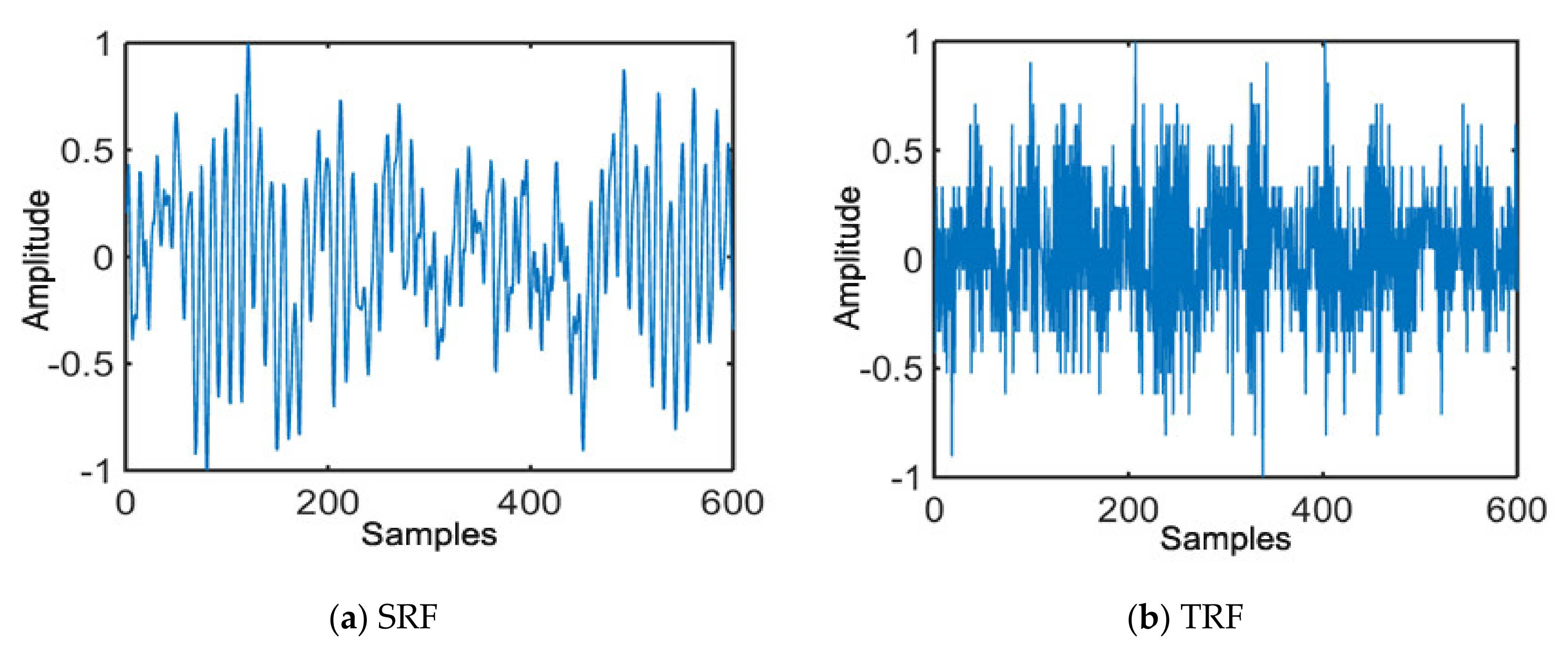
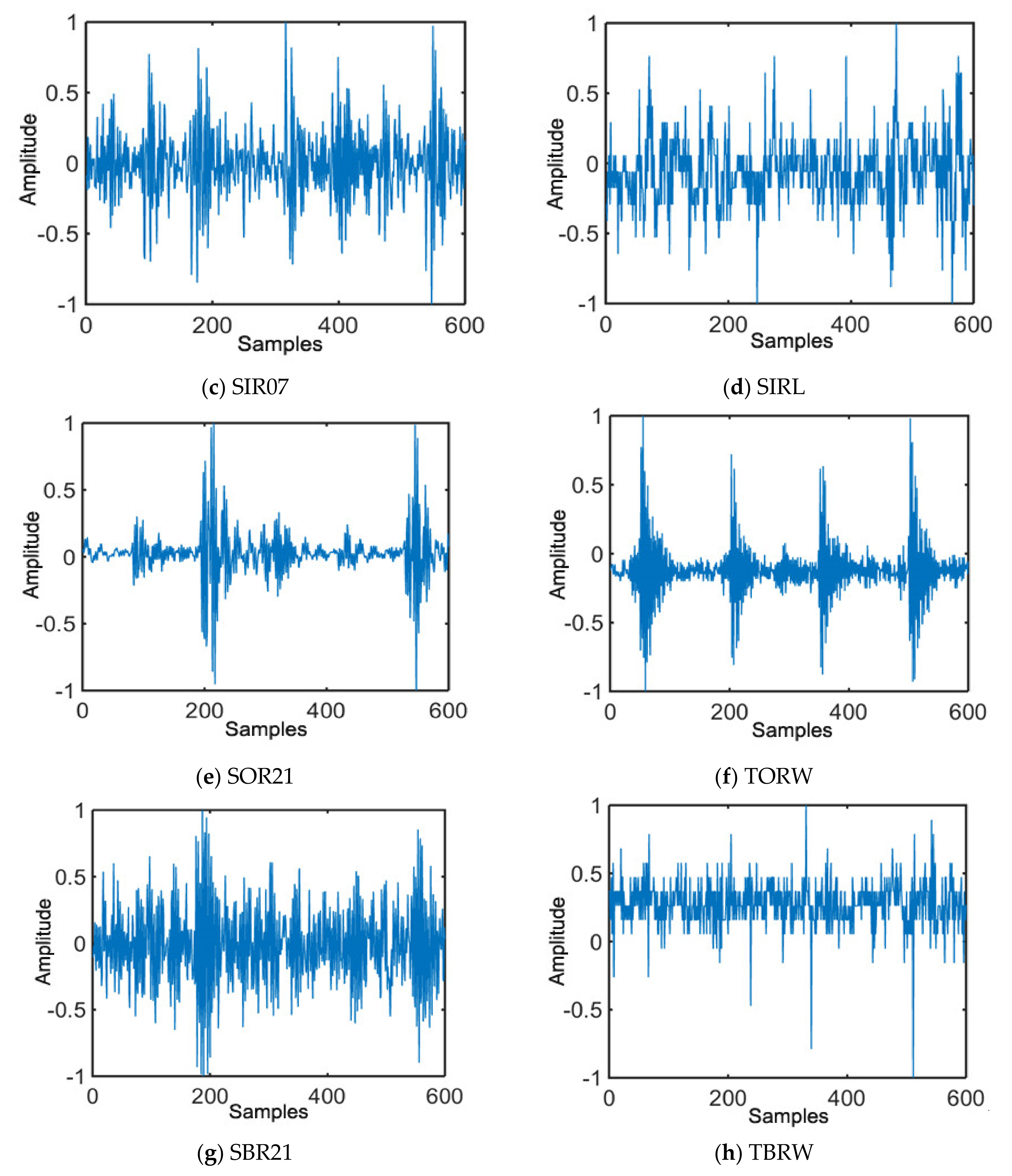
Figure 5 is the diagram of a waveform sample randomly selected from the source domain working condition data set and the target domain data set. The subgraphs a,c,e,g of Figure 5 are the diagrams of waveform samples under source regular family (SRF), fault size of inner ring 0.007 (SIR07), fault size of outer ring 0.021 (SOR21), and fault size of ball roller 0.021 (SBR21). The subgraphs b,d,f,h of Figure 5 shows the waveform samples under target regular family (TRF), slight inner ring fault of lower waveform (SIRL), target outer ring worse (TORW), and target ball roller worse (TBRW). It can be seen that the waveform of the source domain and target domain are greatly different. If the deep learning method is used to diagnose these two domains in the same model, the effect is poor. If two models are trained separately, a lot of time will be spent and resources will be wasted. Therefore, the introduction of transferring learning in practical applications has significance.

5.2. Parameter Selection

Parameter selection is a very important part of the machine learning method. A set of appropriate parameters can effectively improve the performance of fault diagnosis. Because the posterior distribution of deep transfer learning model parameters is often very complex, its closed probability density function cannot be obtained in many cases. A natural way to avoid the problem of estimability is to use the Bayesian method, as a large number of research results show that Bayesian optimization can achieve better performance on the test set and requires fewer iterations than random search. By using the appropriate prior distribution, we can calculate the representative posterior distribution and then use its mean or median to estimate the unknown parameters. In this paper, the parameters of the hidden layer that needs to be inferred is not a fixed unknown, but a random variable that follows a certain distribution, that is, multiple estimates of the random variable follow a certain prior distribution. Combined with the current source domain data, the parameter estimation before is continuously modified, and it is no longer dependent on the source domain data set. This section has discussed the model depth, node number and constraint penalty coefficient $\mathsf{\alpha }$ which have a greater impact on performance. Among them, accuracy is the proportion of all correct predictions (positive and negative). The formula definition is shown in Equation (17), where TP represents a positive class predicted to be a positive class (a correctly predicted positive class), FP represents a negative class predicted to be a positive class, TN represents a negative class predicted to be a negative class, and FN represents a positive class predicted to be a negative class.

$$accuracy=\frac{TP+TN}{TP+TN+FP+FN}$$

(17)

Figure 6 shows the experimental results of accuracy under different layers (1–5) and samples with labels (the number is 1, 2, 4, and 10 respectively) in different target domains, in which the average values of accuracy and time are taken under the four working conditions.

As depicted in Figure 6, with the increase of the number of hidden layers and the number of labeled samples, the fault identification accuracy constantly improved. The more samples with labels, the better the model with excellent performance can be trained, and the more layers, the better the characteristics that can best represent the original data, and the classification ability is improved. However, when the number of hidden layers reached 6, the accuracy rate decreased because the increase of the model complexity will lead to overfitting. In addition, the time of the training model also increased synchronously with the increase of the number of layers. It also can be seen that when the number of hidden layers was 3, the accuracy was basically the same as the number of layers was 4, but the time was much less than the number of layers was 4. Therefore, considering the recognition accuracy and time, the network model structure with the hidden layer number of 3 was appropriate.

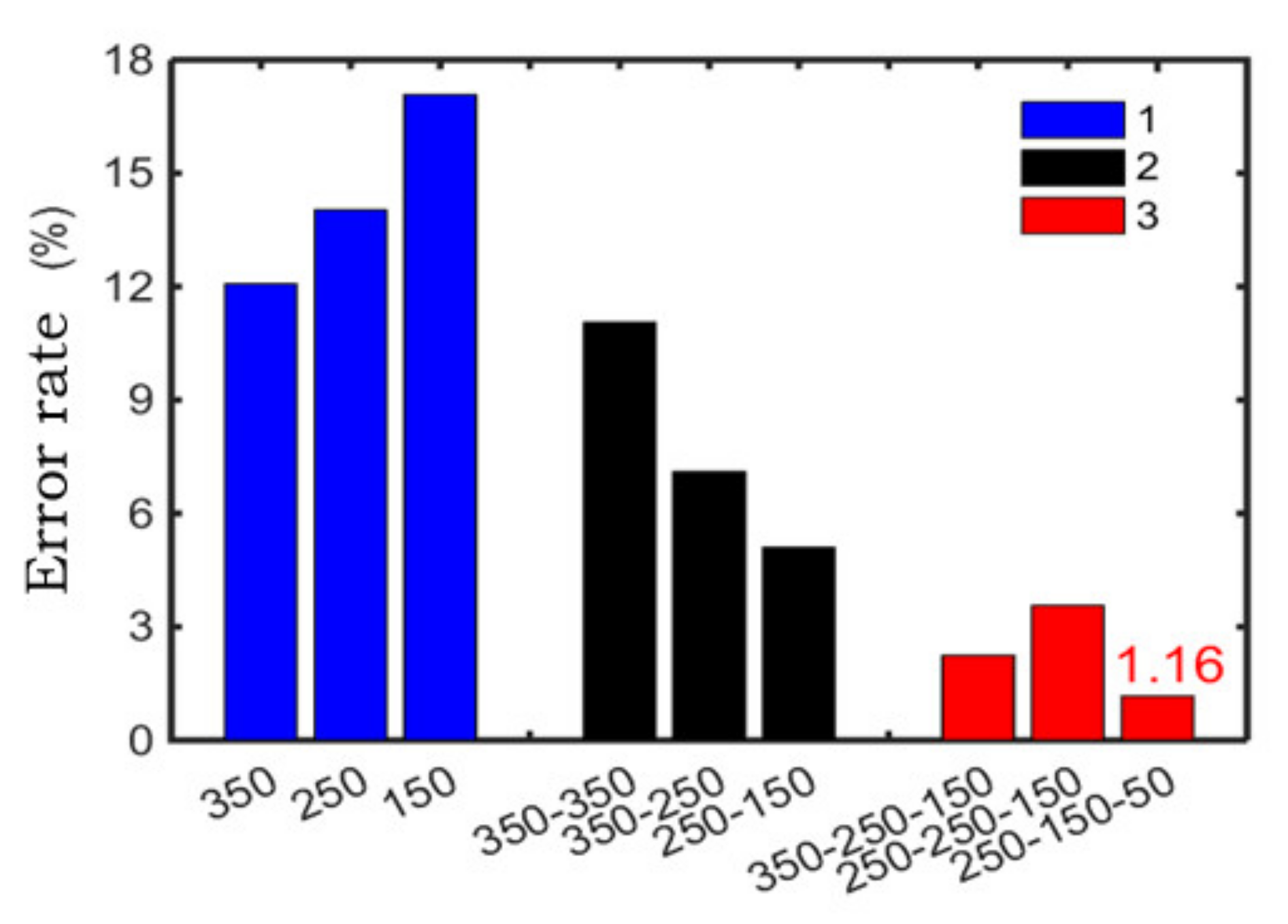
In Figure 7, we find that if the number of hidden layers remains unchanged, the fewer nodes in the next layer, the lower the error rate will be. For example, in the first layer, the second layer and the third layer respectively contained 250, 150, and 50 nodes, and got better results compared with other node configurations. Assuming that the actual output value and the expected output value of each set of data inputted into the hidden layer be $A_i$ and $T_i$ respectively, and the error of each set of data was $\left|A_i-T_i\right|$. m data sets were selected for testing, the average absolute percentage error (APE) of neural network with different number of nodes in each hidden layer is

$$\mathrm{APE}=\frac{1}{m}{\displaystyle \sum }_{i=1}^m\left|\frac{A_i-T_i}{A_i}\right|\ast 100$$

(18)

When m = 30, it is calculated by the Equation (18), the error rate is as low as 1.16%. Therefore, set the network structure to 600–250–150–50–7.

Figure 8 shows the accuracy results under different values. Among them, the value $\alpha$ was calculated according to the rules of {1 × 10^e|e = −5, −4, −3, −2, −1, 0, 1}, and $r$ was set as 0.3 and $\beta$ is 3 through experience and adjustment. It can be found that when the value of $\alpha$ was 0.0001, the best accuracy was 98.84% because the value $\alpha$ can effectively prevent overfitting phenomenon and limit the weight range.

5.3. Experimental and Results Analysis

In order to verify the validity of the method in this paper, it is compared with the basic DSAE and the existing intelligent methods MRSDAE and FE-SSAE-SM. The specific parameters of the TD-DCSAE method were set through experiments and experience. The specific description was as follows: the network structure of DCSAE was [600–250–150–50–7], and the number of iterations for each CSAE was 200. In the fine-tuning stage, the number of iterations for TD-DCSAE was 30, and the parameters $r$, $\beta$ and $\alpha$ were 0.3, 3 and 0.0001, respectively. The network structure of the DSAE model is [600–250–150–50–7]. The number of iterations for each SAE is 200, and the parameters $r$, $\beta$ are 0.3 and 3, respectively. The network structure of the MRSDAE model was [600–250–150–50–7], with 500 iterations, the sparse parameter is 0.1, penalty item was 2, and regular item of L2 norm was 0.005. The network structure of FE-SSAE-SM model was the same as above. The number of iterations was 300, the sparse parameter is 0.5, and the penalty term was 0.1.

Table 3. The accuracy of different methods under different working condition.

Condition	Methods
	TD-DCSAE	DSAE	MRSDAE	FE-SSAE-SM
S1	99.31	87.98	96.04	94.84
S2	98.08	89.94	98.28	96.44
S3	98.26	91.54	96.56	98.00
S4	99.71	89.96	98.60	94.68
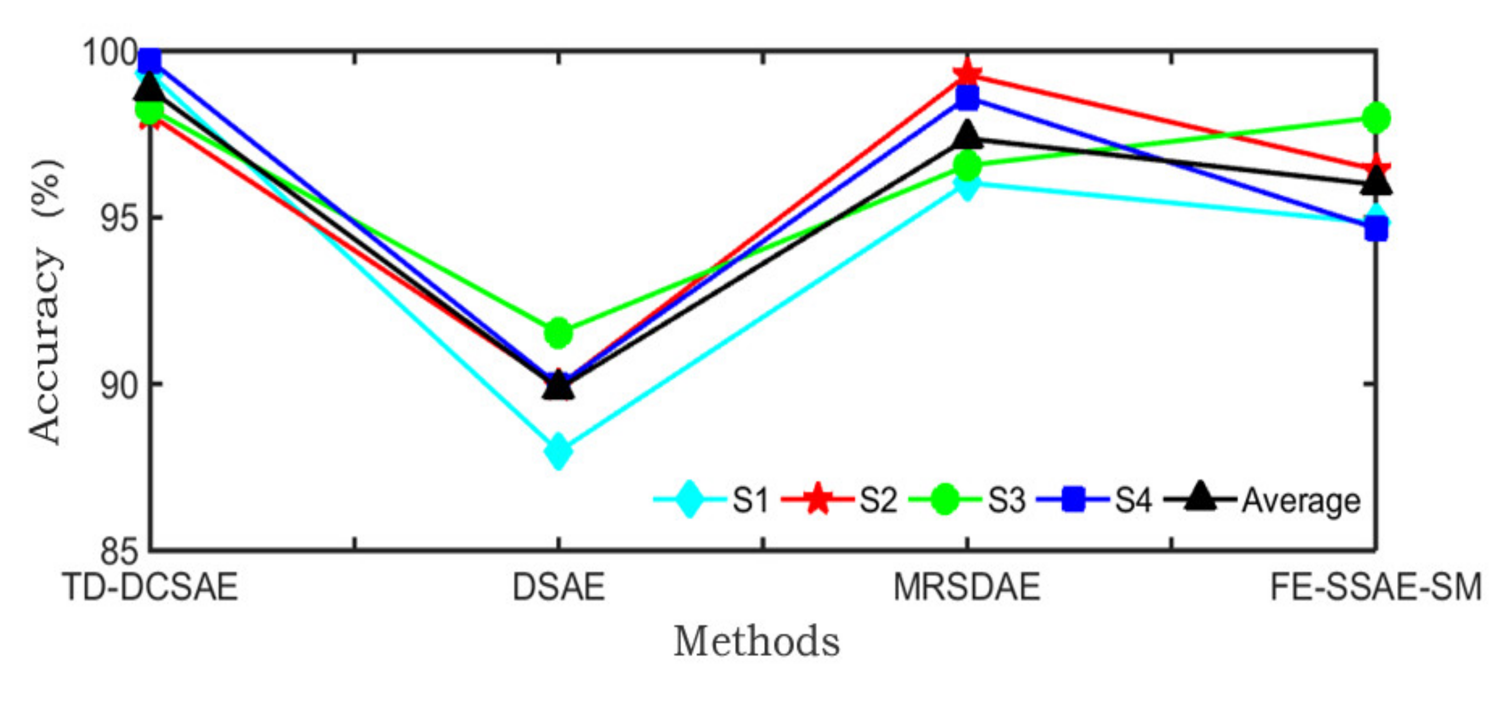
Average accuracy	98.84	89.86	97.37	95.99

shows the accuracy of the TD-DCSAE method and the other three methods under different working conditions, and its accuracy was the average of 10 experiments. Under different working conditions, the TD-DCSAE method achieved the highest values, which were 99.31, 98.08, 98.26, and 99.71%, respectively. Under working condition S1, the accuracy rate was 12 and 3.27% higher than that of DSAE and MRSDAE methods, respectively. Under working condition S4, the accuracy rate is 5.03% higher than that of the FE-SSAE-SM method. The average accuracy was higher than that of DSAE, MRSDAE, and FE-SSAE-SM methods, respectively 8.98, 1.47, and 2.85%.

It is clearly depicted in the Figure 9 that TD-DCSAE method had the highest accuracy in fault classification and is suitable for fault diagnosis of rolling bearings. In

Table 4. The accuracy under a different number of labeled samples in the target domain.

Source Domain(S)-Target Domain (T)	Number of Labeled Samples in the Target Domain
	0.5% (1)	1% (2)	2% (4)	5% (10)	10% (20)	20% (40)	50% (100)
S1-T	87.42	89.36	96.89	97.81	97.94	98.07	98.23
S2-T	87.29	88.91	97.72	97.95	98.07	98.15	98.19
S3-T	87.37	90.19	97.24	97.99	98.12	98.13	98.16
S4-T	85.99	89.61	96.91	97.83	98.10	98.16	98.21
Average accuracy	87.02	89.51	97.19	97.90	98.05	98.13	98.19

, the data sets under S1, S2, S3, and S4 working conditions were respectively taken as the source domain, and the accuracy of model migration was obtained when the number of samples with labels in the target domain was different. Figure 10 shows the average accuracy of the migration under the four working conditions. With the increase of the number of samples with labels in the target domain, the accuracy was gradually improved, but the degree of improvement was also rapidly decreasing. For example, the accuracy of one sample with labels was 87.02%, and that of four samples with labels was 97.19%, an increase of nearly 10 percent. However, when the number of samples with labels increased from 4 to 100, the accuracy only increased 1%. Therefore, the TD-DCSAE method can accurately diagnose the rolling bearings fault with only a small number of labeled target samples.

Table 5. The accuracy of different methods under different number of labeled samples in the target domain.

Method	Number of Labeled Samples in the Target Domain
	0.5% (1)	1% (2)	2% (4)	5% (10)	10% (20)	20% (40)	50% (100)
TD-DCSAE	87.02	89.51	97.19	97.90	98.05	98.13	98.19
DSAE	41.96	46.23	51.68	75.36	82.24	86.88	89.48
BPNN	38.62	41.89	42.99	48.56	54.25	58.23	60.01
SVM	32.95	40.16	66.12	78.65	83.76	88.78	90.58
FE-SSAE-SM	51.94	56.09	68.82	85.51	89.65	91.73	94.19
MRSDAE	54.12	57.23	62.70	87.68	93.20	94.51	95.00

shows the accuracy of different methods in the case of a different number of samples with labels in the target domain. The parameter settings of TD-DCSAE, DSAE, FE-SSAE-SM, and MRSDAE are the same as the above experiments. The network structure of BPNN was [600–1000–7], the learning rate and momentum terms were 0.4 and 0.95, respectively, and the number of iterations was 1000. The Gaussian kernel radius of SVM was 0.65, the penalty coefficient was 8, and the 10-fold cross-validation method was adopted. As can be seen from Table 5 and Figure 11, the accuracy of the above six methods all increased with the increase of the number of samples with labels, but the TD-DCSAE method was superior to the other five methods in the case of the different number of samples with labels, especially when the number of labels was less than 10. For example, when the number of labels was 1, the TD-DCSAE method was nearly 46, 49, 55, 36, and 34 percentage points higher than the DSAE, BPNN, SVM, FE-SSAE-SM, and MRSDAE methods, respectively. In addition, the deep learning method was superior to the shallow learning method, and it can be seen that BPNN and SVM had the lowest accuracy.

6. Conclusions

The method proposed in this paper organically combines the advantages of machine learning and deep learning. First, this model greatly decreases the demand for the data with labels, and significantly reduces the time to mark the data, and avoids the overfitting caused by the training model with less labeled data. Secondly, it is possible to learn multi-task objectives. For each new task, the model does not have to be trained from the beginning, and the cost of later training is very low. Finally, the method can achieve continuous learning so that the model can retain the knowledge learned in the previous task for the next task, improving the stability and generalization of the model. However, this paper only proposes a fault diagnosis method for the label problem of imbalanced data sets. In fact, in practical application, the fault data of the rolling bearings is very limited, and it is very likely that it cannot be collected easily. Under small samples, it is often impossible to build a model. Therefore, how to make a fault diagnosis of rolling bearings under small sample conditions needs to be studied.