Article

Elbows of Internal Resistance Rise Curves in Li-Ion Cells

1
School of Mathematics, University of Edinburgh, Peter Guthrie Tait Road, Edinburgh EH9 3FD, UK
2
Centro de Matemática e Aplicações (CMA), FCT, UNL, Quinta da Torre, 2829-516 Caparica, Portugal
*
Author to whom correspondence should be addressed.
Energies 2021, 14(4), 1206; https://doi.org/10.3390/en14041206
Submission received: 9 January 2021 / Revised: 8 February 2021 / Accepted: 13 February 2021 / Published: 23 February 2021

Abstract

:
The degradation of lithium-ion cells with respect to increases of internal resistance (IR) has negative implications for rapid charging protocols, thermal management and power output of cells. Despite this, IR receives much less attention than capacity degradation in Li-ion cell research. Building on recent developments on ‘knee’ identification for capacity degradation curves, we propose the new concepts of ‘elbow-point’ and ‘elbow-onset’ for IR rise curves, and a robust identification algorithm for those variables. We report on the relations between capacity’s knees, IR’s elbows and end of life for the large dataset of the study. We enhance our discussion with two applications. We use neural network techniques to build independent state of health capacity and IR predictor models achieving a mean absolute percentage error (MAPE) of 0.4% and 1.6%, respectively, and an overall root mean squared error below 0.0061 . A relevance vector machine, using the first 50 cycles of life data, is employed for the early prediction of elbow-points and elbow-onsets achieving a MAPE of 11.5% and 14.0%, respectively.

1. Introduction

Sales of electric vehicles (EVs) and energy storage systems are undergoing a marked growth as battery costs continue to fall and with the introduction of increasingly strict regulations on CO 2 and NO x emissions, deadlines on the decommissioning of fossil fuel power stations and bans on the sale of internal combustion engines. Lithium-ion (Li-ion) batteries are widely deployed in EVs and energy storage systems due to their outstanding characteristics, such as low maintenance requirements, high Coulombic efficiency and market-leading energy density; however, in operation, Li-ion batteries are sensitive to over-charging/discharging, high current stresses, over-temperature and under-temperature. Even when cycled under moderate operating conditions, solid-electrolyte interphase (SEI) layer growth on anodes gradually consumes active material, leading to poor cyclability. Extreme operating conditions will further accelerate ageing processes, potentially resulting in high-risk failure scenarios such as gassing, mechanical cracking of electrodes, internal short circuits and thermal runaway [1,2,3,4,5,6,7,8,9]. Furthermore, the degradation rates of identical chemistry cells differ due to disparities in manufacturing quality and operating conditions [2,10,11,12]. The accurate prognosis of cell degradation is therefore imperative. This is referred to as the State of Health (SOH) of the cell and can be defined with respect to its capacity or its internal resistance (IR). A cell’s capacity fades as its calendar and cycle age increase, and degradation mechanisms take place within the cell that reduce the available lithium inventory and accessible active material in the electrodes [13,14]. Conversely, as the cell is cycled, IR increases due to the thickening formation of the SEI, and the consumption of electrolyte and lithium in this process [1,2].
Given the importance of driving range, capacity is the primary SOH measurement for pure EVs; naturally, capacity-based SOH measurement is less important for hybrid electric vehicles (HEVs), instead, importance is placed on a cell’s ability to supply high operating currents. With the increase of IR, the current deliverability of a cell is diminished, making IR a key SOH measurement for hybrid vehicles. For a given current, increased IR can raise the terminal voltage during the charging phase. As a result, the imposed charging current must be taped down to avoid the battery voltage from exceeding its maximum limit; thus, leading to longer charging times and poor rapid charging ability [9,15,16,17]. In addition, the growth of IR values will incur more heat generation for a given load creating more work for the thermal management system. To the best of our knowledge, the majority of EV manufacturers only provide a battery warranty securing that the capacity shall remain above 70% of its initial value, but ignore a battery warranty based on IR. With a greater understanding of expected IR growth such warranties could be provided. There is thus significant value to be gained from the prognosis of IR growth trends; however, the prediction of IR degradation using data from early cycles remains largely unexplored. There is substantive research e.g., [18,19] conducted for early prediction of capacity but not for IR.
As discussed in-depth in [19], a cell’s capacity does not degrade linearly throughout its lifetime: degradation is path-dependent [20], and a strong association exists between capacity and internal resistance [21]. While the cell’s capacity typically starts to degrade in a linear manner, there eventually comes a point, called the ‘knee-point’, after which the rate of capacity degradation increases considerably [22,23,24,25,26,27,28]. In [19] one can find a review of knee-point identification methods [22,26,28], and, crucially, the additional variable ‘knee-onset’ is introduced (along with an alternative identification mechanism) to provide a useful indication of the beginning of a sharp increase in the capacity degradation trend. However, the corresponding notion of ‘knee-point’ and ‘knee-onset’ in IR degradation curves is absent from the current literature. In this paper, we bridge this gap by addressing the IR rise curve and the corresponding change points: the ‘elbow-onset’ for when the IR curve becomes nonlinear and the midpoint of the accelerated IR increase which we call the ‘elbow-point’.
There are three main contributions of this work. Firstly, at a data pre-processing level, we create an accurate IR predictor utilising machine learning convolutional neural network (CNN) techniques. This predictor is then used to complete the dataset of [29] (for which no IR readings were logged). Secondly, underpinned by the completed dataset, the concepts of elbow-point and elbow-onset points for IR rise curves are proposed along with corresponding identification methods. Thirdly, we showcase a working example of using the predicted and real IR data for the early prediction of elbow-point and elbow-onset using only the first 50-cycles of the cell’s lifespan data.
The rest of this paper is organised as follows. Section 2 introduces the data pool and the data pre-processing approach addressing a missing IR data problem. In Section 3, we propose the elbow-onset and -point concepts and identification algorithms, concluded by a study of the numerous relationships between these quantities. Section 4 presents the relevance vector machine (RVM)-based machine learning approach for the early prediction of elbows. Results, contributions and future work are summarised in Section 5.

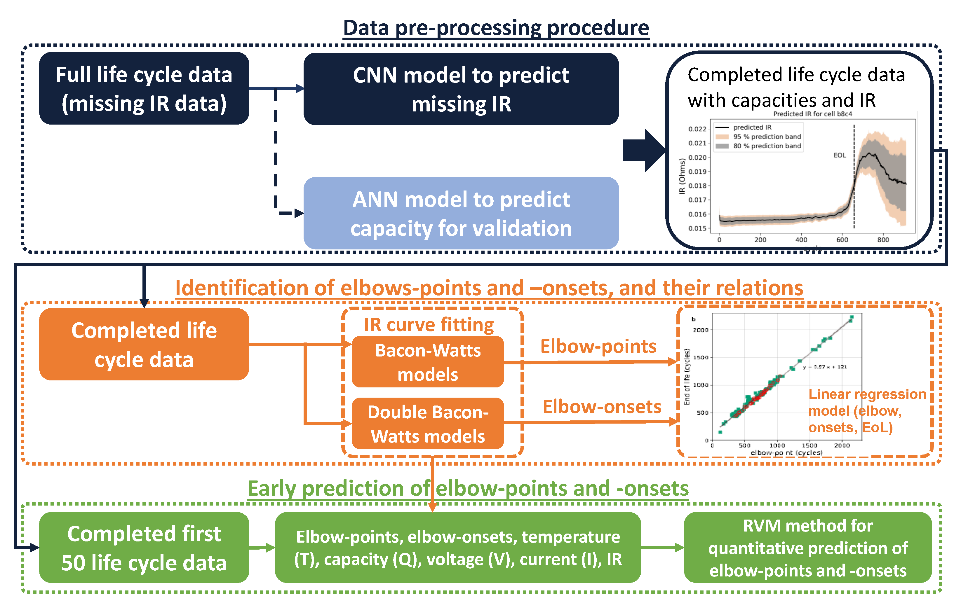
2. Battery Data Framework and Data Pre-Processing Procedures

2.1. Data Description

We mainly work with the datasets of [18,29]. The data, their description and experimental details can be found at https://data.matr.io/1 (accessed on 21 February 2021)—first and second blocks, respectively. Throughout this text, we will refer to the combination of these two datasets as the ‘A123 dataset’. The data pool consists of high-throughput cycling data for eight batches of commercial lithium iron phosphate (LFP)/graphite cells cycled under fast-charging conditions: [18] provides data for three batches of approximately 48 cells each, here referred to as batches 1 to 3 (124 cells in total); Ref. [29] provides data for five batches of cells (233 cells in total), of between 45 and 48 cells each (here referred to as batches 4 to 8); batch 8 has 45 cells. Cell code notation: across the 8 batches of cells in the A123 dataset, we refer to cell Y of batch X as bXcY.
All cells in batches 1, 2 and 3 are cycled to, or close to, their end of life (EOL), defined as 80% of initial capacity, in a temperature-controlled environment with a variety of charge/discharge profiles. It is important to note that, for each individual cell the charge/discharge profile was kept constant from cycle to cycle. Batches 4–7 were only cycled for 100–120 cycles and do not exhibit knees nor reach EOL. Cells in batch 8 were cycled beyond their EOL. The dataset contains both in-cycle and per-cycle measurements. Discharge capacity, temperature, current and charge are logged at an in-cycle level, and per-cycle measurements of capacity, IR and charge time are provided. Data are recorded consistently from the second cycle. Contrary to batches 1–3, batches 4–8 contain no internal resistance measurements. The IR measurements provided are taken at a consistent Ah level of 80% state-of-charge (SOC) relative to nominal capacity. Throughout, we refer to this measurement as the IR of a cell. We note that the IR measurements for batches 1–3 contain a large amount of noise. Severson et al. [18] noted issues with their data logging equipment which in turn affected some tests.

2.2. Data Pre-Processing via a Machine Learning Approach: Completing the Missing IR Data

Our first goal, to increase the scope of our analysis, is to address the missing IR data of batch 8. We draw on machine learning techniques and build an IR prediction model (on the data from batches 1–3) to predict the missing IR data of batches 4–8. Increasing the number of matched capacity-IR curves from 124 pairs to 357 (= 124 + 233). Of these 357 pairs 169 (= 124 + 45) contain measurements up to or past the EOL. This will enhance our later analysis comparing elbows, knees and the EOL, as well as the early prediction of elbows. For statistical reasons, we build a simple yet accurate capacity predictor to test for distributional dissimilarity between batches 1–3 and batches 4–8.

2.2.1. Pre-Processing and Modelling Pipeline

We split the cells of the dataset into training and test sets: grouping by batch so that our test set contains an equal percentage of cells from each batch. As input our capacity and IR prediction models take one charge/discharge cycle of voltage, current and SOC data (the integral of the current from one full cycle). This data was cleaned, standardised to have values between 0 and 1, interpolated using the ‘SciPy’ [30] function ‘interp1d’ to one measurement every four seconds and zero-extended so that the data for each cycle of each cell was of equal length and consistent time step. The median filter, averaging five nearest time instants, was applied to smooth the measurements of capacity and IR prior to prediction.
To design our models for IR and capacity prediction we utilised K-fold cross validation. A validation set of cells was chosen at random from the training set, our models fitted to the remaining training set and evaluated on the validation set throughout training. This step was then repeated K-times with a new validation set and corresponding model. The average performance of the validation sets was used to optimise model design and choice of hyper-parameters. K-fold cross validation is particularly useful when working with small datasets: mitigating the risk of over-fitting a particular validation set [31]. After settling on the model’s architecture and hyper-parameters (described next), a copy of the model was fitted to the whole training set and then evaluated on the test set to calculate performance metrics.

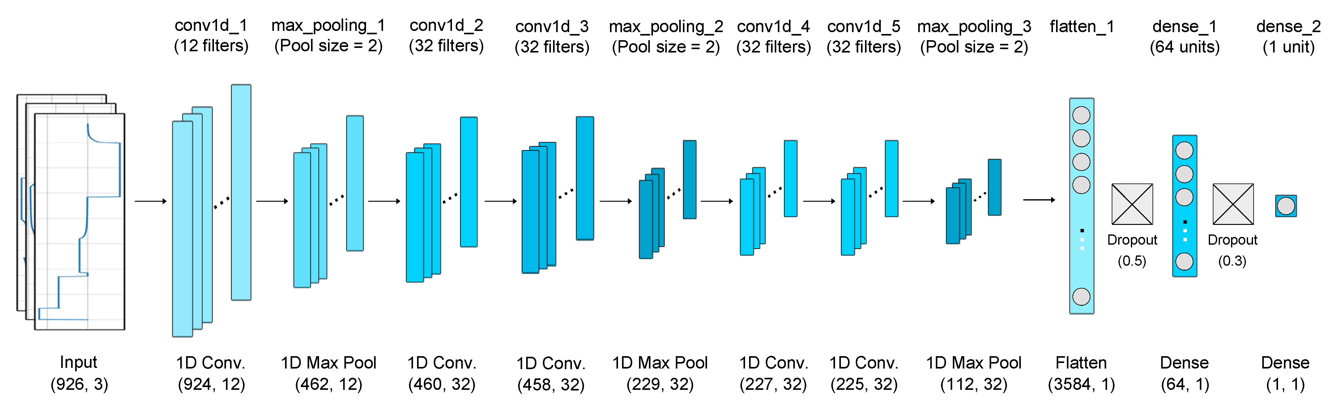
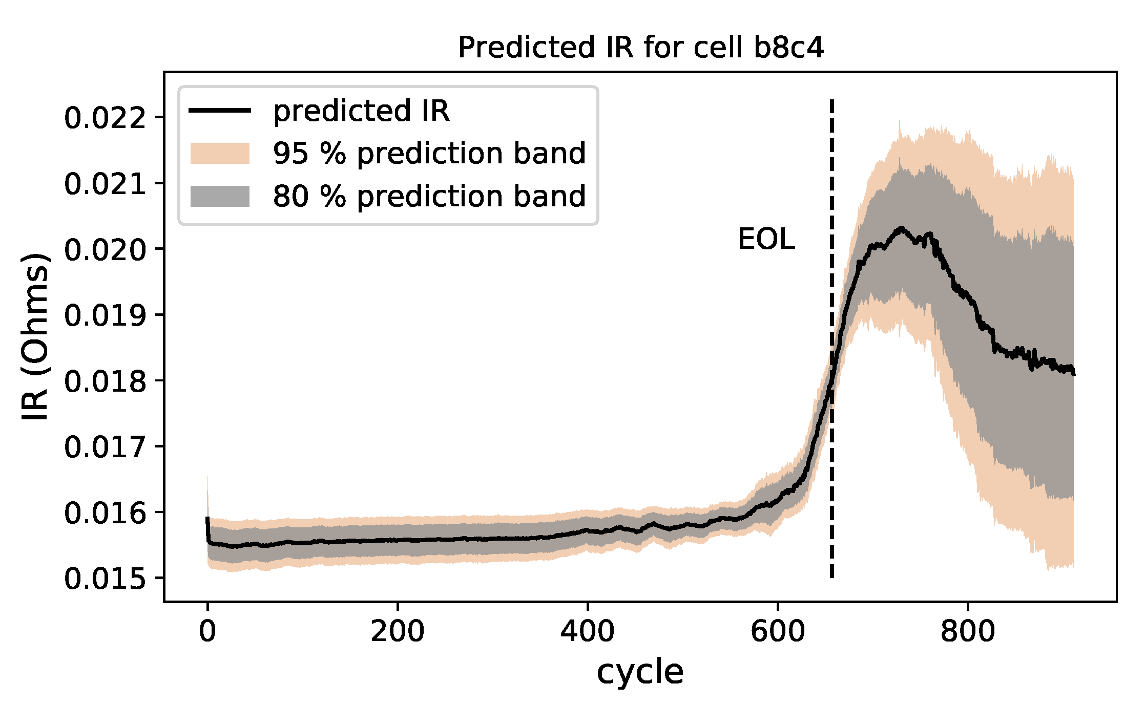
2.2.2. Model for IR Prediction

We propose a model consisting of a convolutional ‘feature extraction’ block followed by two densely connected layers displayed in Figure 1 and described in Table 1. Our model was implemented in Python using TensorFlow via the Keras API [32]. All layer names given in Table 1 refer to the corresponding Keras layers. The model was trained on the data from batches b1–b3 using the adam optimiser for 50 epochs with a batch size of 526 and the mean absolute error—Equation (1)—as its loss function.
The machine learning performance scores selected for this work are the mean absolute error (MAE), mean absolute percentage error (MAPE) and root mean square error (RMSE) defined as follows. For y the vector of true values and y ^ the vector of predicted values
MAE ( y , y ^ ) = 1 n samples i = 1 n samples | y i ^ y i | , MAPE ( y , y ^ ) = 100 % n samples i = 1 n samples | y i ^ y i | y i ,
and RMSE ( y , y ^ ) = 1 n samples i = 1 n samples ( y ^ i y i ) 2 .
Our model’s performance metrics for IR prediction can be found in Table 2. We are unaware of works using the A123 dataset for IR estimation. Nonetheless, the estimation of IR has been addressed for other datasets [33,34,35,36,37,38,39]. We obtain an RMSE of 0.00035 and an MAPE of 1.6 % which is low (if nominally compared with capacity estimation accuracy in the literature).

2.2.3. Validation Step via a Model for Capacity Prediction

We have shown that our model for IR prediction is effective on batches 1–3. To see if we can trust the predictions that this model makes on batches 4–8 we check for non-similarity between the datasets. We do this by extrapolating on capacity—a variable present for all batches. This is a standard process in imputation (simple or multiple). To this end, we utilise a simple feed-forward neural network consisting of three densely-connected layers: the first two layers containing 32 neurons with the rectified linear unit (ReLU) activation function and the final layer consisting of a single neuron with a linear activation. The model was trained for 100 epochs with a batch size of 512 using the adam optimiser and the mean squared error as its loss function. During training, a dropout of 0.2 was used between the middle and last layer. Trained on all of the data from batches 1–3 and tested on batches 4–8, the model obtained the performance metrics displayed in Table 3 with an MAPE of 0.51 %. This test gives us confidence that both datasets [18,29] are indeed not dissimilar.
The prediction of capacity (and SOH) is of wider interest than our discussion of elbows, so we briefly compare these results with those found in the literature. We point to Table 1 in [40] (MAPE and RMSE error given) and Table 2 in [41] (error type not given) for a review/comparative work on capacity estimation. We cannot directly compare our results, as the data is different. However, from a strictly numerical point of view, our RMSE of 0.0095 and MAPE 0.51% errors for capacity (Table 3) are lower than the values of [40] (Table 1)—for a fair comparison, one would need to test the varying approaches on a common dataset.

2.2.4. Predicting the Missing IR Data

In order to address the missing data issue, we trained the IR model on batches 1–3 multiple times and an ensemble of these models was used to predict on batches 4–8. This predicted IR data is available at https://doi.org/10.7488/ds/2957 (accessed on 21 February 2021). Figure 2 shows the IR for sample cell b8c4 and we strongly emphasise to the reader that the extrapolation of the IR data past EOL (80% capacity) is, as fully expected, not reliable; this stems from the limitation of the training dataset (batches 1–3) with data only up to the EOL. Prediction outside that range of input data is not reliable as can be seen in Figure 2 where we observe a strong widening in the prediction intervals past the EOL. The prediction intervals provided throughout the text are calculated in a frequentist manner. A given model is fitted to data multiple times and performance metrics/predictions recorded. The empirical average and variance-value of predictions are calculated and under the assumption of normality one uses those values to produce prediction intervals (at any given probability quantile level q, e.g., in Figure 2 we have q = 95 % and q = 80 % ).

2.2.5. Algorithmic Framework

The proposed algorithmic framework takes full advantage of machine learning-based approaches to solve the missing IR data problem in the raw data pool allowing the generation of artificial IR data to complete the life cycle data. The predicted IR data can be used for elbow-point and -onset identification and is able to assist the early prediction of the elbow-point and elbow-onset in IR curves.
The schematic framework of the algorithms is illustrated in Figure 3. Section 2 introduces the data pre-processing procedure, where a CNN-based predictor has been trained on the data from batches 1–3 to predict the missing IR of batches 4–8. For validation, a capacity estimator was trained to test for dissimilarity between the two datasets. In Section 3, using the completed data we confirm significant linear relationships between knee/elbow-points, -onsets and EOL. Further tests are carried out in Section 4 relating to the early prediction of elbow-points and -onsets. In particular, the straightforward RVM-based quantitative method is applied for the early prediction of elbows.

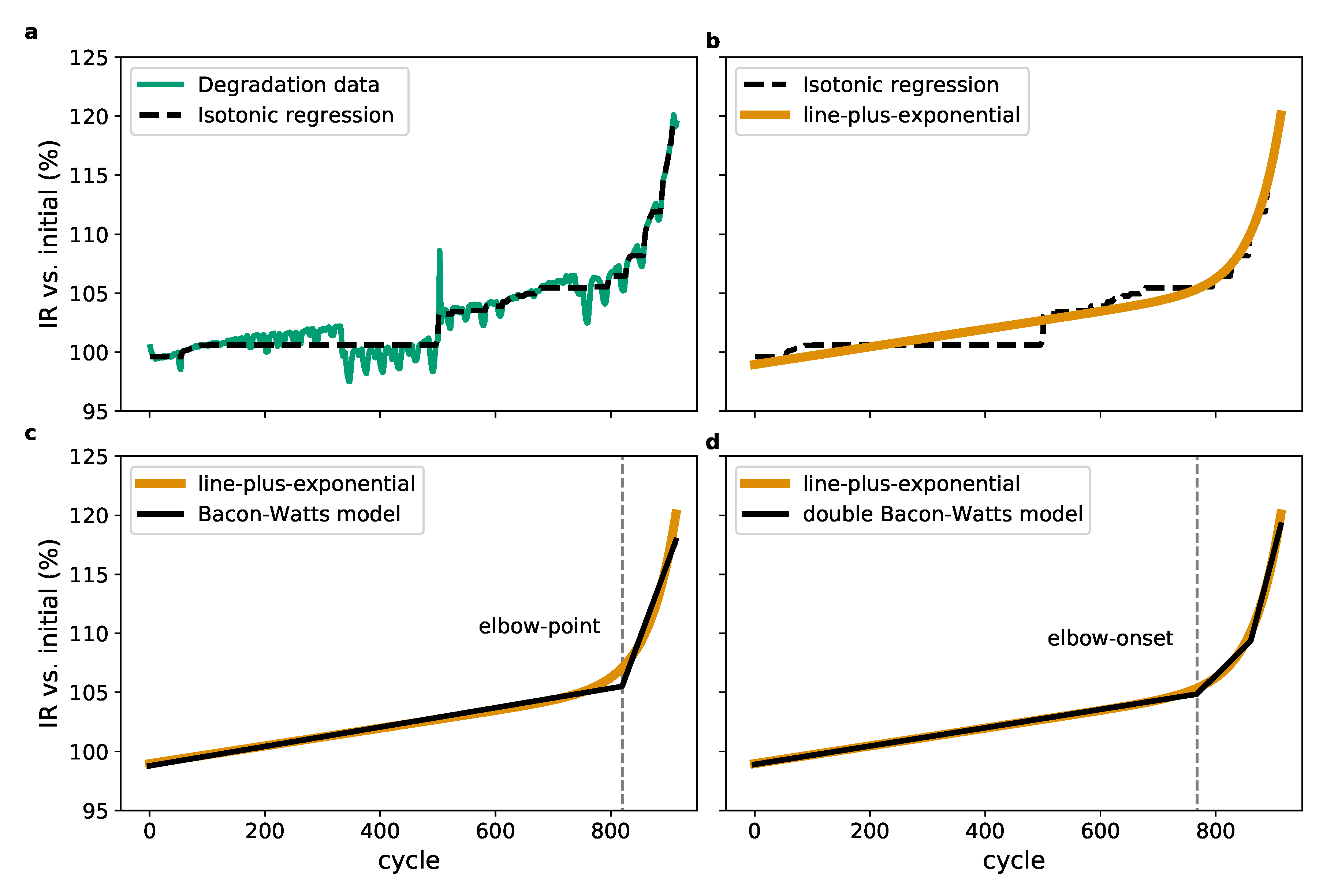
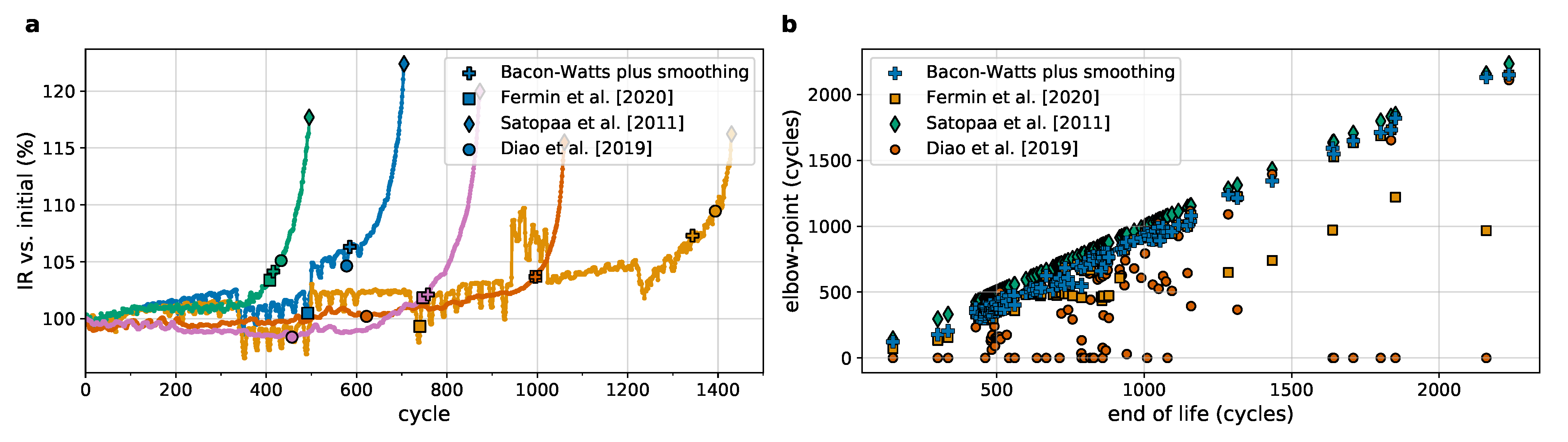
3. Identification of Elbows, Knees and Their Relations

3.1. Methodology

Fermín et al. [19] proposed the use of the Bacon–Watts (Equation (5)) and the double Bacon–Watts model (Equation (6)) for the identification of knee-point and knee-onset, respectively. We will use the same basic methodology, with the addition of several steps to account for noise in the data and potential sigmoid behaviour. The high level of noise present in the IR data, see Figure 4a and Figure 5a, prevents the Bacon–Watts model from neatly fitting the data, and this is overcome via a smoothing step as described in Algorithm 1 (block 1) below. We report that this noise also causes issues for the alternative knee identification methods proposed in [19,22,26], see Figure 5. In addition, we observed sigmoid-type capacity fade curves for some cells in batch 8, and hence, we employ a subroutine to isolate the knee/elbow identification from the right-most plateau. We present first the algorithm and afterwards reason its several steps.
Algorithm 1 ‘Smoothed Bacon–Watts’: Identification of knee/elbow-point and -onset
Block 1: Data smoothing.
  • Fit isotonic regression to (capacity/IR degradation) lifespan data (across the full curve).
  • Determine data-truncation cycle-point n * :
    (a)
    Fit (3) (Asymmetrical sigmoidal) to isotonic regression curve,
    (b)
    Find cycle-number n * : cycle at which 2nd derivative of fitted (3) changes sign, else last cycle in series.
  • Fit (4) (line-plus-exponential) to isotonic regression curve up to cycle n * .
Block 2: Identification.
4.
Fit Bacon–Watts model (5) to (4). Identify knee/elbow-point.
5.
Fit double Bacon–Watts model (6) to (4). Identify knee/elbow-onset.
The isotonic regression step, Step 1, solves several issues: it annuls the behaviour of capacity increase or IR decrease across the first few cycles and removes the influence of sharp movements where the IR decreases or increases due to measurement errors. From first principles, our choice reflects the fact that the electrochemical degradation mechanisms within the cell are irreversible. For a given load and set of ambient conditions, IR increase may be caused by the thickening of the SEI on the anode which irreversibly consumes lithium and electrolyte. Additionally, IR increase can be caused by a loss of anode and cathode material which can result from many factors, such as electrode particle cracking and loss of electrical contact as a result of mechanical expansion/contraction during cycling, corrosion of current collectors at low cell voltage and binder decomposition at high cell voltage. These same mechanisms also lead to an irreversible reduction in capacity and, as such, the monotonicity of the model is reflective of the real-world evolution of a cell’s capacity over its lifespan. The isotonic regression is performed using the Scikit-learn Python package [42] and the procedure is described in [43].
Throughout the manuscript, and the following equations, the generic ε variable denotes the errors/residuals of its associated model, indicated as a superscript, and is a normal random variable with zero mean and finite (unknown) variance.
The asymmetrical sigmoidal fitting step, Step 2. The asymmetrical sigmoidal (‘ a s ’) model is described by Equation (3)
Y a s = d + a d 1 + x c b m + ε a s ,
where a and d associate to the top and bottom plateau of the curve respectively, b controls the slope between plateaus, m the level of asymmetry and c determines the inflexion point. For given data, the constants are estimated by straightforward least-squares estimation (similarly for subsequent parametric models).
In several cells from batch 8, we observe a sigmoid-type capacity fade curve where, after passing the knee and then degrading linearly for some time, the degradation approaches a plateau (e.g., cell b8c4). To isolate the detection of knees/elbows from this behaviour, we propose the fitting of the asymmetrical sigmoidal model to then truncate the data before said plateau (point n * ) via the 2nd derivative truncation rule.
The final smoothing step, Step 3, involves fitting the parametric line-plus-exponential (‘ l e ’) model of Equation (4) to the isotonic data (from Step 2) up to cycle n * . This idea can be traced back to [44] (Section 2.2.1) under the name of ‘Exponential/linear hybrid model’—[36,45] discuss other parametric models. The line-plus-exponential is described by the following model:
Y l e = β 0 + β 1 x + β 2 exp ( λ x θ ) + ε l e ,
where β 0 , β 1 and β 2 control the intersection point and slope of the line, and the size of the exponential, respectively. The quantity λ controls the ‘speed’ of the exponential and θ controls where the impact of the exponential starts. The main motivation for model (4) is that for many cells, the degradation of IR is very close to linear until close to the elbow-onset followed by a sharp elbow-point.
For the identification of the knee/elbow-point, Step 4, we use the Bacon–Watts model. Fermín et al. [19] (Equation (1)) describe the Bacon–Watts (‘ b w ’) model (5) as a two straight-line relationships around the transition point x 1 :
Y b w = α 0 + α 1 ( x x 1 ) + α 2 ( x x 1 ) tanh { ( x x 1 ) / γ } + ε b w ,
where α 0 , α 1 and α 2 control the slopes of the intersecting lines and the intercept-weigh of the leftmost segment respectively and γ controls the abruptness of the transition. We fix γ as a small value to obtain an abrupt transition. After optimisation, the fitted value of x 1 is defined as the knee/elbow-point.
The identification of the knee/elbow-onset, Step 5, is performed by the double Bacon–Watts model (‘ d b w ’) (6) (also [19] Equation (2)) modifying Bacon–Watts to identify two transition points, concretely:
Y d b w = α ^ 0 + α ^ 1 ( x x 0 ) + α ^ 2 ( x x 0 ) tanh { ( x x 0 ) / γ ^ } + α ^ 3 ( x x 2 ) tanh { ( x x 2 ) / γ ^ } + ε d b w ,
as in Equation (5), the parameters α ^ i and x j are estimated and γ ^ is chosen as a small value to produce abrupt transitions at x 0 and x 2 . The knee/elbow-onset is defined as the change point x 0 .
Figure 4 displays the output of Algorithm 1 applied to the IR curve of cell b1c29 (non-predicted data). Elbow-point and its onset are identified, and the smoothing steps are illustrated showing the fitted isotonic regression and line-plus-exponential model against the input data (for this cell, Step 2 yields n * as the final cycle number). Figure 5 displays the performance of other known algorithms for knee identification applied to the elbow identification problem. We find that [19,22,26]’s algorithms are too sensitive to noise to provide consistent identification results. Our approach addresses the noise issue allowing for coherent elbow identification. From a statistical point of view, any identification approach will be affected by the noise in the data; thus, the identified elbows will be less exact than the identified knees, for which the data is much smoother. For comparison, the non-parametric bootstrap procedure was used to calculate 95% confidence intervals (CI) for the knee/elbow-points and -onsets identified by Algorithm 1. The average CI’s width was 24 cycles for the elbow-point, 4 cycles for the knee-point, 35 cycles for the elbow-onset and 5 cycles for the knee-onset; this difference is a direct consequence of the noise present in the IR data. Finally, Algorithm 1 applied to knee identification recovers fully the results of [19] (we omit these results).
Zhang et al. [28] report for a dataset of nickel-manganese-cobalt cells that the knee-point appeared at between 90–95% nominal capacity; in [19], it was reported that the knee-point, for batches 1–3 of the A123 dataset, appeared on average at 95% nominal capacity and the knee-onset at 97.1% nominal capacity, with an average gap of 108 cycles between the knee and its onset. We report that, for the A123 dataset batches 1, 2, 3 and 8, on average, the elbow-onset appears at 103.0 % initial IR ( 93.6 % nominal capacity) and the elbow-point at 104.7 % initial IR ( 91.3 % nominal capacity), with the elbow-onset and its point on average 52 cycles apart; on average, both elbows appear after the knee-point. These reported figures are calculated from the smoothed exponential curve as described in Algorithm 1.

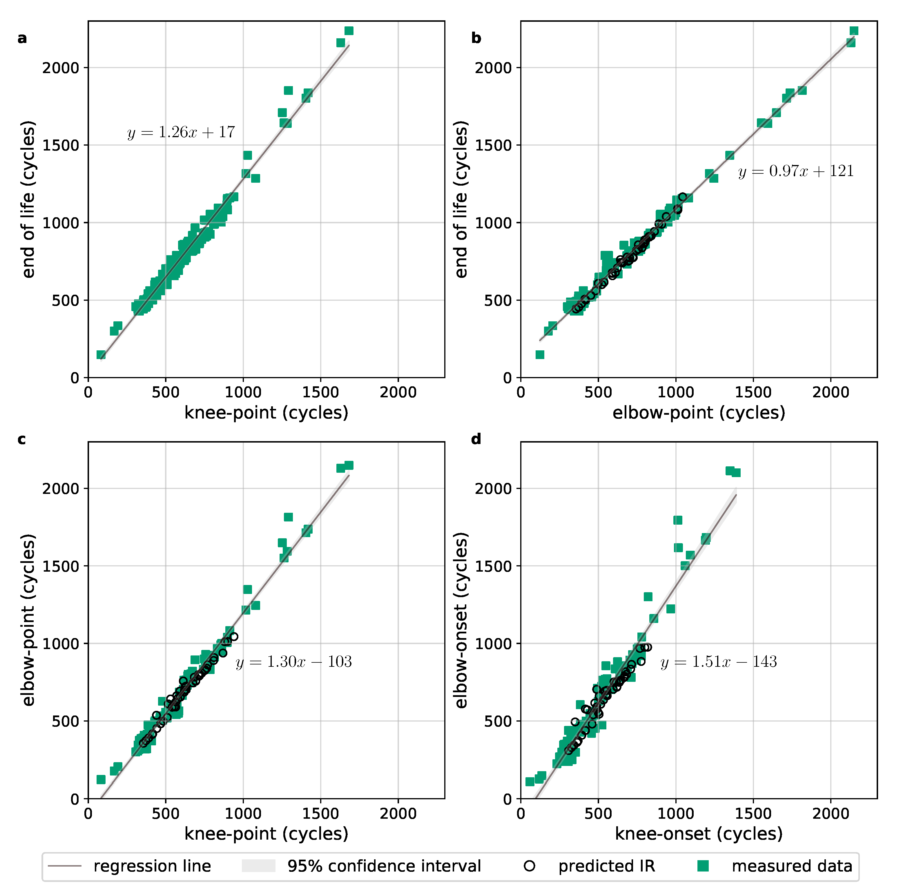
3.2. Linear Relations

Figure 6 illustrates the strong linear relationships observed between the calculated knee/elbow-points and the EOL, making it possible to estimate each point given a measurement or prediction of another point(s). These linear relations are obtained using a standard linear regression model y = c 0 + c 1 x + ε , where y denotes the dependent variable, x the independent variable, ε represents the residuals, and c 0 and c 1 control the intercept and slope of the linear model, respectively. The obtained coefficient values along with their confidence intervals are presented in Table 4, where the knee relations agree with those found in [19] (Table 1).
We present the linear relationships obtained when including the predicted IR data. From viewing Figure 6, comparing the green squares and black circles, the reader will appreciate that their inclusion did not significantly influence the linear relationship obtained. This observation lends a second layer of credibility to the predicted IR data: the elbows displayed in the predicted IR match closely with what one would expect given the linear relationships observed on batches 1–3.

4. Early Prediction of Elbows

A real-word challenge is how to predict the trajectory of IR growth, e.g., the elbow points in IR curves as to detect early signs of unacceptable degradation. For example, to filter out cell production lots that will exhibit faster increases in IR or to schedule HEV battery replacement/maintenance. We complement the previous section in scope of the findings of [19] (Section 3). We apply the quantitative knee prediction algorithm developed there to the early prediction of elbows without any additional optimisation, i.e., ‘as is’. A full description of the model and feature extraction process can be found in [19] and Supplementary Material; however, we provide a brief overview. It is outside the scope of this paper to revisit the early prediction of knees.
The quantitative prediction of the elbows is performed by a RVM [46], a type of linear regression mechanism, taking features extracted from the early life of the cells. The feature extraction process takes as input the first 50-cycles of the available per-cycle and in-cycle measurements (capacity, IR, charging-times, voltage, current, temperature) and draws on time-series analysis to calculate a vast collection of summary statistics without input from domain expertise (see [19] Supplementary Figure S5). Then, a sequential feature selection funnel is deployed to select around 100 features to train the RVM [19] (Supplementary Figures S6 and S7). When using batch 8 the input IR is the predicted IR from Section 2.2.4—the cases with/without batch 8 are distinguished. The model is trained on data from all but one cell and tested on the remaining cells (leave-one-out framework); this process is independently repeated such that each cell is used for testing once. The performance metrics displayed in Table 5 are the average of the test performances.
The resultant early predictions are reported in Table 5, where two points should be made salient. Firstly, on elbows vs. knees prediction, when compared to [19], the model performs worse predicting elbows than when predicting knees: MAPE 13.8 % vs. 12.0 % , elbow-onset vs. knee-onset, and MAPE 10.7 % vs. 9.4 % , elbow-point vs. knee-point—overall, the elbow prediction is up to 2% worse when compared with knee prediction. This lower accuracy in elbow (vs. knee) prediction was expected as the input IR measurements are much noisier than the capacity measurements, and hence, the identification of elbows is inherently less exact, which in turn affects the predictive performance—as argued in Section 3.1, the confidence intervals for the elbow identification are significantly wider than those for the knees. Due to this higher noise in the elbows, when predicting elbows from input data, the relationship between input data and elbows will be weaker/noisier than when predicting the knees.
Secondly, the inclusion of the predicted IR data leads to a marginally worse average performance of our model: the MAPE worsens by 0.2% for the elbow-onset prediction and by less than 0.8% for the elbow-point prediction, see Table 5. This critically showcases that the generated IR data may be used for the prediction of elbows—which we emphasise was an input feature to the RVM.
From a methodological point of view, we employed the simple RVM algorithm of [19] in a direct manner: without any additional optimisation to take into account the noisier IR data or the predicted IR data. This was a choice to prove that the generated IR data can be used for early prediction. There is indeed room for future improvements in the early prediction of IR elbows and such is left for future research. Lastly, increasing the number of cells displaying elbows by prediction to 169 (= 124 + 45) will benefit approaches that are highly dependent on the size of a dataset.

5. Conclusions and Future Work

In this original work, the IR rise curve of Li-ion cells is characterised by the novel concept of ‘elbow-point’ and ‘elbow-onset’; a generalist identification algorithm is then proposed. The proposed approach is able to handle not only measurement noises but also sigmoid-type patterns in capacity fade and IR rise curves. The findings highlight significant linear relationships between EOL, capacity knee-point/IR elbow-point and capacity knee-onset/IR elbow-onset for the data under study.
Two machine learning-related goals were achieved. The first, part of the data pre-processing step, draws on neural network techniques to build independent IR and capacity SOH predictors achieving a small MAPE of 1.6% and 0.4% respectively—these results are of wider general interest. The proposed IR estimator has been deployed to complete an existing cell cycling dataset with missing IR measurements resulting in a well-rounded life cycle dataset encompassing both capacity and IR data. The generated data is publicly available. Such datasets can be used for both identification and the early prediction of elbows in IR curves. We then provided an illustrative example for such an early predictor of IR elbows. Furthermore, the cells with predicted IR are shown to be usable for the early prediction of elbows: resulting in only slightly worse average performance than when they are excluded (the MAPE worsens by less than 0.8%).
The methods of elbow identification and prediction, in this work, have commercial value to battery manufacturers as well as end users such as fleet managers and energy storage utility operators. Accurate early forecasting of the IR elbows will allow manufacturers to set appropriate performance and lifetime warranties for their products. Additionally, elbow forecasting allows battery users to accurately and conveniently schedule battery maintenance and replacement, or adjust the duty cycle to accommodate the reduced performance of the battery pack as it degrades.
In the future, the accuracy of the early prediction will be enhanced. Multiple dimensions of inputs encompassing the predicted IR data and other measurements will be used to train the model with an improved tolerance for noisy data. Overall, elbow identification and elbow early prediction can be used to influence the design of the thermal management system: accounting for the additional heat dissipated by cells as they approach their EOL. A study comparing the relations between knee/elbow-onset and -point across more datasets is left to future work.

Supplementary Materials

The predicted internal resistance dataset created to complement batches 4–8, those of the [29] dataset, is available online at https://doi.org/10.7488/ds/2957 (accessed on 21 February 2021).

Author Contributions

C.S. and R.G. provided implementation and Machine learning expertise. C.S., G.d.R. and S.L. performed data analysis, modelling and interpretation of results. S.L. provided domain expertise. All authors edited and reviewed the manuscript. G.d.R. supervised the work and funding acquisition. All authors have read and agreed to the published version of the manuscript.

Funding

This project was funded by an industry-academia collaborative grant EPSRC EP/R511687/1 (PIV003), Data-driven prediction of battery life cycle—Knees and Elbows, funded by EPSRC and University of Edinburgh program Impact Acceleration Account (IAA); Dukosi Ltd, Edinburgh acts as the industrial partner. G.d.R. acknowledges support from the Fundaç a ˜ o para a Ci e ^ ncia e a Tecnologia (Portuguese Foundation for Science and Technology) through the project UIDB/00297/2020 (Centro de Matemática e Aplicaç o ˜ es CMA/FCT/UNL).

Acknowledgments

G.d.R. would like to thank the colleagues from Dukosi Ltd. for the helpful discussions. All authors thank W. Dhammika Widanage (Warwick uni, WMG group), Weihan Li and Philipp Dechent (RWTH Aachen University), Vanda Inácio (U. of Edinburgh) and Euan McTurk (Plug Life Consulting Ltd.) for the helpful discussions.

Conflicts of Interest

There are no conflicts to declare. Public declaration of Software Disclosure with Edinburgh Innovation/University of Edinburgh, Invention Id ERI2020/129.

References

  1. Gilbert, J.A.; Shkrob, I.A.; Abraham, D.P. Transition metal dissolution, ion migration, electrocatalytic reduction and capacity loss in lithium-ion full cells. J. Electrochem. Soc. 2017, 164, A389–A399. [Google Scholar] [CrossRef]
  2. Waldmann, T.; Wilka, M.; Kasper, M.; Fleischhammer, M.; Wohlfahrt-Mehrens, M. Temperature dependent ageing mechanisms in lithium-ion batteries—A Post-Mortem study. J. Power Sources 2014, 262, 129–135. [Google Scholar] [CrossRef]
  3. Matsuda, T.; Ando, K.; Myojin, M.; Matsumoto, M.; Sanada, T.; Takao, N.; Imai, H.; Imamura, D. Investigation of the influence of temperature on the degradation mechanism of commercial nickel manganese cobalt oxide-type lithium-ion cells during long-term cycle tests. J. Energy Storage 2019, 21, 665–671. [Google Scholar] [CrossRef]
  4. Li, J.; Downie, L.E.; Ma, L.; Qiu, W.; Dahn, J. Study of the failure mechanisms of LiNi0. 8Mn0. 1Co0. 1O2 cathode material for lithium ion batteries. J. Electrochem. Soc. 2015, 162, A1401–A1408. [Google Scholar] [CrossRef]
  5. Uitz, M.; Sternad, M.; Breuer, S.; Täubert, C.; Traußnig, T.; Hennige, V.; Hanzu, I.; Wilkening, M. Aging of tesla’s 18650 lithium-ion cells: Correlating solid-electrolyte-interphase evolution with fading in capacity and power. J. Electrochem. Soc. 2017, 164, A3503–A3510. [Google Scholar] [CrossRef] [Green Version]
  6. Campbell, I.D.; Marzook, M.; Marinescu, M.; Offer, G.J. How Observable Is Lithium Plating? Differential Voltage Analysis to Identify and Quantify Lithium Plating Following Fast Charging of Cold Lithium-Ion Batteries. J. Electrochem. Soc. 2019, 166, A725–A739. [Google Scholar] [CrossRef]
  7. Park, K.J.; Hwang, J.Y.; Ryu, H.H.; Maglia, F.; Kim, S.J.; Lamp, P.; Yoon, C.S.; Sun, Y.K. Degradation Mechanism of Ni-Enriched NCA Cathode for Lithium Batteries: Are Microcracks Really Critical? ACS Energy Lett. 2019, 4, 1394–1400. [Google Scholar] [CrossRef] [Green Version]
  8. Birkl, C.R.; Roberts, M.R.; McTurk, E.; Bruce, P.G.; Howey, D.A. Degradation diagnostics for lithium ion cells. J. Power Sources 2017, 341, 373–386. [Google Scholar] [CrossRef]
  9. Liu, Q.; Du, C.; Shen, B.; Zuo, P.; Cheng, X.; Ma, Y.; Yin, G.; Gao, Y. Understanding undesirable anode lithium plating issues in lithium-ion batteries. RSC Adv. 2016, 6, 88683–88700. [Google Scholar] [CrossRef]
  10. Dubarry, M.; Baure, G.; Devie, A. Durability and reliability of EV batteries under electric utility grid operations: Path dependence of battery degradation. J. Electrochem. Soc. 2018, 165, A773–A783. [Google Scholar] [CrossRef]
  11. Somerville, L.; Bareño, J.; Trask, S.; Jennings, P.; McGordon, A.; Lyness, C.; Bloom, I. The effect of charging rate on the graphite electrode of commercial lithium-ion cells: A post-mortem study. J. Power Sources 2016, 335, 189–196. [Google Scholar] [CrossRef] [Green Version]
  12. Gao, Y.; Jiang, J.; Zhang, C.; Zhang, W.; Ma, Z.; Jiang, Y. Lithium-ion battery aging mechanisms and life model under different charging stresses. J. Power Sources 2017, 356, 103–114. [Google Scholar] [CrossRef]
  13. Hendricks, C.; Williard, N.; Mathew, S.; Michael, P. A failure modes, mechanisms, and effects analysis (FMMEA) of lithium-ion batteries. J. Power Sources 2015, 297, 113–120. [Google Scholar] [CrossRef] [Green Version]
  14. Friedrich, F.; Strehle, B.; Freiberg, A.T.S.; Kleiner, K.; Day, S.J.; Erk, C.; Piana, M.; Gasteiger, H.A. Capacity Fading Mechanisms of NCM-811 Cathodes in Lithium-Ion Batteries Studied by X-ray Diffraction and Other Diagnostics. J. Electrochem. Soc. 2019, 166, A3760–A3774. [Google Scholar] [CrossRef]
  15. Rodrigues, M.T.F.; Kalaga, K.; Trask, S.E.; Dees, D.W.; Shkrob, I.A.; Abraham, D.P. Fast Charging of Li-Ion Cells: Part I. Using Li/Cu Reference Electrodes to Probe Individual Electrode Potentials. J. Electrochem. Soc. 2019, 166, A996–A1003. [Google Scholar] [CrossRef]
  16. Ahmed, S.; Bloom, I.; Jansen, A.N.; Tanim, T.; Dufek, E.J.; Pesaran, A.; Burnham, A.; Carlson, R.B.; Dias, F.; Hardy, K.; et al. Enabling fast charging - A battery technology gap assessment. J. Power Sources 2017, 367, 250–262. [Google Scholar] [CrossRef]
  17. Yang, X.G.; Zhang, G.; Ge, S.; Wang, C.Y. Fast charging of lithium-ion batteries at all temperatures. PNAS 2018, 115, 7266–7271. [Google Scholar] [CrossRef] [Green Version]
  18. Severson, K.; Attia, P.; Jin, N.; Perkins, N.; Jiang, B.; Yang, Z.; Chen, M.; Aykol, M.; Herring, P.; Fraggedakis, D.; et al. Data-driven prediction of battery cycle life before capacity degradation. Nat. Energy 2019, 4, 1–9. [Google Scholar] [CrossRef] [Green Version]
  19. Fermín, P.; McTurk, E.; Allerhand, M.; Medina-Lopez, E.; Anjos, M.F.; Sylvester, J.; dos Reis, G. Identification and machine learning prediction of knee-point and knee-onset in capacity degradation curves of lithium-ion cells. Energy AI 2020, 1, 100006. [Google Scholar] [CrossRef]
  20. Raj, T.; Wang, A.A.; Monroe, C.W.; Howey, D. Investigation of Path Dependent Degradation in Lithium-Ion Batteries. Batter. Supercaps 2020, 3, 1377–1385. [Google Scholar] [CrossRef]
  21. Bao, Y.; Dong, W.; Wang, D. Online internal resistance measurement application in lithium ion battery capacity and state of charge estimation. Energies 2018, 11, 1073. [Google Scholar] [CrossRef] [Green Version]
  22. Diao, W.; Saxena, S.; Han, B.; Pecht, M. Algorithm to Determine the Knee Point on Capacity Fade Curves of Lithium-Ion Cells. Energies 2019, 12, 2910. [Google Scholar] [CrossRef] [Green Version]
  23. Neubauer, J.; Pesaran, A. The ability of battery second use strategies to impact plug-in electric vehicle prices and serve utility energy storage applications. Lancet 2011, 196, 10351–10358. [Google Scholar] [CrossRef]
  24. Ecker, M.; Nieto, N.; Käbitz, S.; Schmalstieg, J.; Blanke, H.; Warnecke, A.; Sauer, D.U. Calendar and cycle life study of Li(NiMnCo)O2-based 18650 lithium-ion batteries. J. Power Sources 2014, 248, 839–851. [Google Scholar] [CrossRef]
  25. Han, X.; Ouyang, M.; Lu, L.; Jianqiu, L. Cycle Life of Commercial Lithium-Ion Batteries with Lithium Titanium Oxide Anodes in Electric Vehicles. Energies 2014, 7, 4895–4909. [Google Scholar] [CrossRef] [Green Version]
  26. Satopaa, V.; Albrecht, J.; Irwin, D.; Raghavan, B. Finding a “kneedle” in a haystack: Detecting knee points in system behavior. In Proceedings of the 2011 31st International Conference on Distributed Computing Systems Workshops, Minneapolis, MN, USA, 20–24 June 2011; pp. 166–171. [Google Scholar]
  27. Schuster, S.F.; Bach, T.; Fleder, E.; Müller, J.; Brand, M.; Sextl, G.; Jossen, A. Nonlinear aging characteristics of lithium-ion cells under different operational conditions. J. Energy Storage 2015, 1, 44–53. [Google Scholar] [CrossRef]
  28. Zhang, C.; Wang, Y.; Gao, Y.; Wang, F.; Mu, B.; Zhang, W. Accelerated fading recognition for lithium-ion batteries with Nickel-Cobalt-Manganese cathode using quantile regression method. Appl. Energy 2019, 256, 113841. [Google Scholar] [CrossRef]
  29. Attia, P.M.; Grover, A.; Jin, N.; Severson, K.A.; Markov, T.M.; Liao, Y.H.; Chen, M.H.; Cheong, B.; Perkins, N.; Yang, Z.; et al. Closed-loop optimization of fast-charging protocols for batteries with machine learning. Nature 2020, 578, 397–402. [Google Scholar] [CrossRef] [Green Version]
  30. Virtanen, P.; Gommers, R.; Oliphant, T.E.; Haberland, M.; Reddy, T.; Cournapeau, D.; Burovski, E.; Peterson, P.; Weckesser, W.; Bright, J.; et al. SciPy 1.0: Fundamental Algorithms for Scientific Computing in Python. Nat. Methods 2020, 17, 261–272. [Google Scholar] [CrossRef] [Green Version]
  31. Kohavi, R. A study of cross-validation and bootstrap for accuracy estimation and model selection. In Proceedings of the 14th International Joint Conference on Artificial Intelligence (IJCAI’95), Montreal, QC, Canada, 20–25 August 1995; Volume 2, pp. 1137–1143. [Google Scholar]
  32. Chollet, F. Keras: The Python Deep Learning Library. 2018. Available online: https://keras.io (accessed on 21 February 2021).
  33. Liang, K.; Zhang, Z.; Liu, P.; Wang, Z.; Jiang, S. Data-driven ohmic resistance estimation of battery packs for electric vehicles. Energies 2019, 12, 4772. [Google Scholar] [CrossRef] [Green Version]
  34. Remmlinger, J.; Buchholz, M.; Meiler, M.; Bernreuter, P.; Dietmayer, K. State-of-health monitoring of lithium-ion batteries in electric vehicles by on-board internal resistance estimation. J. Power Sources 2011, 196, 5357–5363. [Google Scholar] [CrossRef]
  35. Guha, A.; Patra, A. State of health estimation of lithium-ion batteries using capacity fade and internal resistance growth models. IEEE Trans. Transp. Electrif. 2017, 4, 135–146. [Google Scholar] [CrossRef]
  36. Tseng, K.H.; Liang, J.W.; Chang, W.; Huang, S.C. Regression models using fully discharged voltage and internal resistance for state of health estimation of lithium-ion batteries. Energies 2015, 8, 2889–2907. [Google Scholar] [CrossRef] [Green Version]
  37. Giordano, G.; Klass, V.; Behm, M.; Lindbergh, G.; Sjöberg, J. Model-based lithium-ion battery resistance estimation from electric vehicle operating data. IEEE Trans. Veh. Technol. 2018, 67, 3720–3728. [Google Scholar] [CrossRef]
  38. Saha, B.; Goebel, K.; Poll, S.; Christophersen, J. Prognostics methods for battery health monitoring using a Bayesian framework. IEEE Trans. Instrum. Meas. 2009, 58, 291–296. [Google Scholar] [CrossRef]
  39. Zhang, J.; Zhang, X. A Novel Internal Resistance Curve Based State of Health Method to Estimate Battery Capacity Fade and Resistance Rise. In Proceedings of the 2020 IEEE Transportation Electrification Conference & Expo (ITEC), Chicago, IL, USA, 23–26 June 2020; pp. 575–578. [Google Scholar]
  40. Qin, T.; Zeng, S.; Guo, J. Robust prognostics for state of health estimation of lithium-ion batteries based on an improved PSO–SVR model. Microelectron. Reliab. 2015, 55, 1280–1284. [Google Scholar] [CrossRef]
  41. Ng, M.F.; Zhao, J.; Yan, Q.; Conduit, G.J.; Seh, Z.W. Predicting the state of charge and health of batteries using data-driven machine learning. Nat. Mach. Intell. 2020, 2, 161–170. [Google Scholar] [CrossRef] [Green Version]
  42. Pedregosa, F.; Varoquaux, G.; Gramfort, A.; Michel, V.; Thirion, B.; Grisel, O.; Blondel, M.; Prettenhofer, P.; Weiss, R.; Dubourg, V.; et al. Scikit-learn: Machine Learning in Python. J. Mach. Learn. Res. 2011, 12, 2825–2830. [Google Scholar]
  43. Chakravarti, N. Isotonic median regression: A linear programming approach. Math. Oper. Res. 1989, 14, 303–308. [Google Scholar] [CrossRef]
  44. Hu, C.; Ye, H.; Jain, G.; Schmidt, C. Remaining useful life assessment of lithium-ion batteries in implantable medical devices. J. Power Sources 2018, 375, 118–130. [Google Scholar] [CrossRef]
  45. Tang, X.; Liu, K.; Wang, X.; Gao, F.; Macro, J.; Widanage, W.D. Model migration neural network for predicting battery aging trajectories. IEEE Trans. Transp. Electrif. 2020, 6, 363–374. [Google Scholar] [CrossRef]
  46. Bishop, C.M. Sparse Kernel Machines. In Pattern Recognition and Machine Learning; Springer: Berlin, Germany, 2006; Chapter 7; pp. 325–353. [Google Scholar]
Figure 1. Schematic of machine learning model for internal resistance (IR) prediction.
Energies 14 01206 g001
Figure 2. The predicted IR data for cell b8c4 are given by the black continuous line and is formed from the average of 20 predictions. We display 80% and 95% prediction intervals. Beyond the intuition of extrapolation, these intervals show that predictions past the EOL (capacity) should not be trusted.
Energies 14 01206 g002
Figure 3. Graphical abstract for the proposed algorithmic framework.
Energies 14 01206 g003
Figure 4. Steps of Algorithm 1 applied to the internal resistance degradation curve of cell b1c29 (non-predicted data). (a), step 1. (b), step 3. (c), step 4. (d), step 5. Step 2 is omitted as it has no impact here: n * is chosen as the final cycle number. The width of the 95% confidence interval (computed by the non-parametric bootstrapping procedure) for the elbow-point of this curve is 23 cycles, and for the elbow-onset it is 38 cycles.
Energies 14 01206 g004
Figure 5. (a), Comparison of elbow-points obtained with Algorithm 1, [19]’s Bacon–Watts, maximum curvature and slope changing ratio methods on a sample of cells from the A123 dataset (from left to right b2c34, b1c30, b3c15, b3c1, b1c3). (b), Comparison of elbow-points for all cells in the A123 dataset. One expects to see a linear relationship between EOL and elbow-point; of the methods compared only Algorithm 1 and the algorithm of Satopaa et al. [2011] recover a linear relationship reliably, however, by examining plot (a), we see that Satopaa’s algorithm selects the end point as the elbow.
Energies 14 01206 g005
Figure 6. (a), Linear regression model linking the knee-point to end of life. (b), elbow-point to end of life. (c), knee-point to elbow-point. (d), knee-onset to elbow-onset. Every linear model is presented with a 95% confidence band on the plotted regression line; all linear relations here are calculated from the A123 dataset enriched with the predicted IR data for batch 8. Elbow points derived from the predicted IR data are highlighted as open black circles; the reader will appreciate that their inclusion did not significantly influence the linear regression results obtained.
Energies 14 01206 g006
Table 1. Proposed architecture of convolutional neural network (CNN) model for prediction of IR. Hyper-parameters are given in the format: filters, kernel size, activation for conv1d layers; pool size for max_pooling; dropout rate for dropout; nodes, activation for dense layers.
Layer NameInput SizeHyper-ParametersOutput Size
conv1d_1 926 × 3 12, 3, ReLU 924 × 12
max_pooling_1 924 × 12 2 462 × 12
conv1d_2 462 × 12 32, 3, ReLU 460 × 32
conv1d_3 460 × 32 32, 3, ReLU 458 × 32
max_pooling_2 458 × 32 2 229 × 32
conv1d_4 229 × 32 32, 3, ReLU 227 × 32
conv1d_5 227 × 32 32, 3, ReLU 225 × 32
max_pooling_3 225 × 32 2 112 × 32
flatten_1 112 × 32 -3584
dropout_13584 0.5 3584
dense_1358464, ReLU64
dropout_264 0.3 64
dense_2641, linear1
Table 2. Average performance of model to predict IR with 95 % prediction intervals.
RMSEMAPE (%)
TrainTestTrainTest
IR 0.00029 ± 6.2 × 10 5 0.00035 ± 5.0 × 10 5 1.19 ± 0.22 1.60 ± 0.24
Table 3. Average performance of capacity model trained on batches 1–3 tested on batches 4–8, with 95 % prediction intervals.
RMSEMAPE (%)
TrainTestTrainTest
Capacity 0.0053 ± 4.2 × 10 3 0.0095 ± 4.6 × 10 3 0.37 ± 0.30 0.51 ± 0.26
Table 4. Coefficients of four linear regression models relating the knee-point (a) and the elbow-point (b) to the end of life, the knee-point to the elbow-point (c) and the knee-onset to elbow-onset (d), respectively. The p-values for β 1 were computed using the Wald test, and the small values allow the rejection of the null hypothesis that a linear relationship does not exist. The 95% confidence intervals for the estimated coefficients are calculated via bootstrapping. The coefficient of determination, R 2 , of these linear regression models is (a) 0.9822 , (b) 0.9896 , (c) 0.9818 and (d) 0.9520 ; all close to 1, showing that the fitted models explain the observed data well.
(a) Knee-Point to EOL(b) Elbow-Point to EOL
CoefficientEstimatep-valueCoefficientEstimatep-value
Intercept ( β 0 ) 17 ± 21 Intercept ( β 0 ) 121 ± 11
Slope ( β 1 ) 1.26 ± 0.04 4.0 × 10 148 Slope ( β 1 ) 0.97 ± 0.02 4.5 × 10 162
EOL = 1.26 × knee-point + 17EOL = 0.97 × elbow-point + 121
(c) Knee-Point to Elbow-Point(d) Knee-Onset to Elbow-Onset
CoefficientEstimatep-valueCoefficientEstimatep-value
Intercept ( β 0 ) 103 ± 28 Intercept ( β 0 ) 143 ± 42
Slope ( β 1 ) 1.30 ± 0.05 3.6 × 10 147 Slope ( β 1 ) 1.51 ± 0.08 4.5 × 10 112
elbow-point = 1.30 × knee-point − 103elbow-onset = 1.51 × knee-onset − 143
Table 5. Result of RVM regressor for elbow-onset (a) and elbow-point (b) when predictions are made from the first 50 cycles. The 90 % confidence intervals (CI) were calculated via bootstrapping. The entry ‘With b8?’ refers to results computed with (‘Yes’) and without (‘No’) the inclusion of the artificially predicted IR data of batch 8.
(a) Elbow-Onset Prediction(b) Elbow-Point Prediction
With b8?MetricScoreCI ( α = 0.1 )With b8?MetricScoreCI ( α = 0.1 )
NoMAE (cycles)89.1[77.0, 101.8]NoMAE (cycles)76.3[64.5, 88.6]
MAPE (%)13.8[12.4, 15.3] MAPE (%)10.7[9.5, 12.0]
YesMAE (cycles)91.3[79.4, 104.0]YesMAE (cycles)83.4[72.8, 94.6]
MAPE (%)14.0[12.6, 15.5] MAPE (%)11.5[10.4, 12.8]
Publisher’s Note: MDPI stays neutral with regard to jurisdictional claims in published maps and institutional affiliations.

