1. Introduction
With the increase of global wind power installations from only about 24 GW in 2001 to about 651 GW by the end of 2019 [
1] a growing number of wind farms are erected in regions with complex terrain. Moreover, these wind farms are getting larger and include several hundreds of wind turbines. The requirement for accurate site assessment studies is growing due to increasing price pressure with decreasing subsidies. On-site measurements, numerical simulations for transferring the winds from the measurement location to the planned wind turbine sites as well as long-term referencing data-sets for the evaluation of wind variability on the long-term scale among others are subject to cost-benefit calculations. Large investments rely on a precise estimate of the wind conditions prior to the erection of these wind farms. In particular, the erection of ever-increasing wind farms in complex terrain creates new challenges on the modeling of site conditions to transfer the wind conditions from the measurement to the planned turbine positions. In the past, strongly simplified approaches such as the linearized WAsP (wasp wind atlas analysis and application program) model [
2] were commonly used for the transfer of site conditions in the terrain. However, this approach is reaching the edges of its validity with increasing terrain complexity [
3,
4]. If the terrain complexity is higher—commonly expressed in terms of a ruggedness index that describes the steepness of the terrain [
5]—higher-fidelity numerical methods such as Reynolds-Averaged-Navier-Stokes (RANS) models are often applied to model the flow modification due to the terrain features (e.g., [
6]).
In recent years, this RANS modeling approach was widely enhanced with the focus on phenomena, that are relevant for site conditions such as atmospheric stratification, forests or also the calibration based on measurement data (e.g., [
7,
8,
9,
10]). With the increasing availability of computational power, the RANS method is nowadays also applied in industrial wind energy applications (e.g., [
11]). In case of very complex terrain features such as cliffs and escarpments even turbulence resolving methods such as hybrid RANS/Large-Eddy Simulation (LES) methods (e.g., [
12,
13]) or LES (e.g., [
14,
15]) are sometimes applied for studying flow features at wind energy sites. However, due to the significantly higher computational costs, full site assessment studies that cover the full range of wind conditions that occur over the lifetime of the turbines can so far not be done using these turbulence-resolving high-fidelity methods. For larger sites or sites in regions with strong regional-scale effects such as land-sea-breezes or gap flows through very large valleys, meso-scale models are used to resolve the impact of these effects. These models offer resolutions in the order of a few kilometres and are well-suited to resolve the large-scale flow or flows in non-complex terrains, in particular offshore (e.g., [
16]). Nowadays, in combination with a micro-scale downscaling, meso-scale models are commonly applied in wind energy applications for the generation of wind atlases (e.g., [
4,
17,
18]).
The coupling of meso- and micro-scale models is a recent topic of interest from an academic and industrial point of view [
19,
20]. The most consistent method is to simply increase the resolution of the meso-scale modeling approach by adding additional nests (e.g., [
21]). However, the time dependency of this approach in addition to the extra nests makes the simulations computationally expensive. Therefore, a climatology based on time series, that is commonly referred to as “dynamical downscaling”, cannot be modeled with this approach and the currently available computational power. The dynamical downscaling is generally not limited to using the same model on all scales. The time series output from a meso-scale model can also be used as forcing terms for a micro-scale model (e.g., [
22]). A second—less computationally expensive—downscaling approach is the “statistical downscaling”. In this approach, the wind climate at a site is analyzed in terms of a relatively low number of classes/states that are commonly defined in terms of e.g., wind direction, atmospheric stability and/or wind speed (e.g., [
23,
24]).
The probability of each state is computed based on its occurrence in the site’s wind climate and only the most relevant states are simulated. The full wind climate is, afterwards, reconstructed from weighting the simulation results obtained for the relevant states. The wind climate is directly extracted from a meso-scale grid cell on-site, or a virtual climatology is applied, interpolating meso-scale data from several grid cells before downscaling (e.g., [
25]). This method significantly reduces the amount of computational power needed. A combination of the statistical and the dynamical downscaling approaches can be achieved by simulating certain site-specific relevant diurnal cycles that can then be used to reconstruct the full wind climate. Consequently, this method is typically referred to as “statistical dynamical downscaling”. The reconstruction of the wind climate by diurnal cycles might be appropriate for sites with dominant diurnal cycles, however, at many locations, the synoptic conditions dominate and thus the applicability remains questionable or many diurnal cycles need to be simulated. A more detailed review on meso–micro coupling methods in wind energy applications is given in [
19].
When different meso- and micro-scale models are coupled in terms of statistics, the coupling can be done based on a single point of the meso-scale model in space or through including the impact of different neighboring meso-scale points that cover the region of interest. A coupling method of this latter type was introduced more recently by [
26,
27], applying it to dispersion modeling and wind energy siting studies, respectively. A recent introduction to the field is a combination of different neighboring meso-scale points in a dynamical downscaling [
28]. The micro-scale simulations include meso-scale simulation data in the inflow conditions. Similar to other dynamic downscaling methodologies numerical constrains prohibit the use for wind climate applications. In this contribution, the method from [
26,
27] is generalized and also enhanced in the context of wind energy applications. Moreover, instead of focusing on critical flow situations, this study applies and evaluates the method on a wind climate of a full year for a benchmark site with a large database for evaluation. We further propose a methodology to include micro-scale models with stratification. In general, the method has the advantage of being computationally efficient and it is based on pre-calculated micro-scale and meso-scale simulations and thus well suited for industrial applications. With increasing computational power, downscaled wind climatologies are more and more entering the field of industrial applications.
The objectives of this paper are to (i) present a fast approach for meso–micro downscaling to an industry-applicable CFD modeling framework, (ii) to test this approach and its sensitivity for single—in terms of meso-scale variability—critical flow situations, (iii) evaluate the meso–micro downscaling approach in terms of site assessment by the use of long-term mast data means, applying evaluation metrics (statistical bias (BIAS) and root-mean-square error (RMSE)). In
Section 2 we present the general downscaling concept in detail.
Section 3 describes the benchmark site Rödeser Berg (complex terrain site in central Germany), followed by the simulation specifications in
Section 4.
Section 5 focuses on the proof of concept and analysis in regard to the objectives stated above. The conclusions that were drawn from our study are presented in
Section 6. Moreover, an outlook to further research is provided to the reader.
2. Downscaling Methodology
This section describes the downscaling methodology used in this study. It is fully applied to micro- and meso-scale numerical simulation data that is generated independently from each other and therefore it is an advanced postprocessing tool that can be applied to any meso–micro modeling setup. For this reason the description here is kept as general as possible. The specific model setup used in this study is given in
Section 4.
In the downscaling process, each of the two models adds an essential ingredient: the meso-scale model provides data that includes the impact of the regional scale while the micro-scale model brings the local orographic effects into the framework. Being a transient model, the meso-scale model will also provide information on relevant time-depending meso-scale and synoptic effects such as frontal passages or winds due to large-scale convection. The meso-scale model data is standard output so that for regions where wind atlases are publicly available, like Europe with its New European Wind Atlas (NEWA) [
4], these data can be used.
The data from the micro-scale model should be an average wind field such as a field from RANS or an averaged wind field from LES. To represent a full wind climate several wind fields (defined by inflow wind directions) need to be available from the micro-scale model. Only one specific micro-scale simulation resulting in a specific wind speed at a target position and target height is done per wind direction sector. From this simulation, speed-up factors are calculated by comparing micro-scale and meso-scale wind speeds. This process significantly reduces the amount of computing time needed. The method can be enhanced by a simulation of different atmospheric conditions. So that for example the wind climate is reduced to 36 sectors and three different stratification conditions—resulting in 108 micro-scale model simulations.
2.1. General Concept
In general, in the downscaling process, time-dependent data from the meso-scale model simulations around the site are combined/scaled with the local wind field from the micro-scale model.
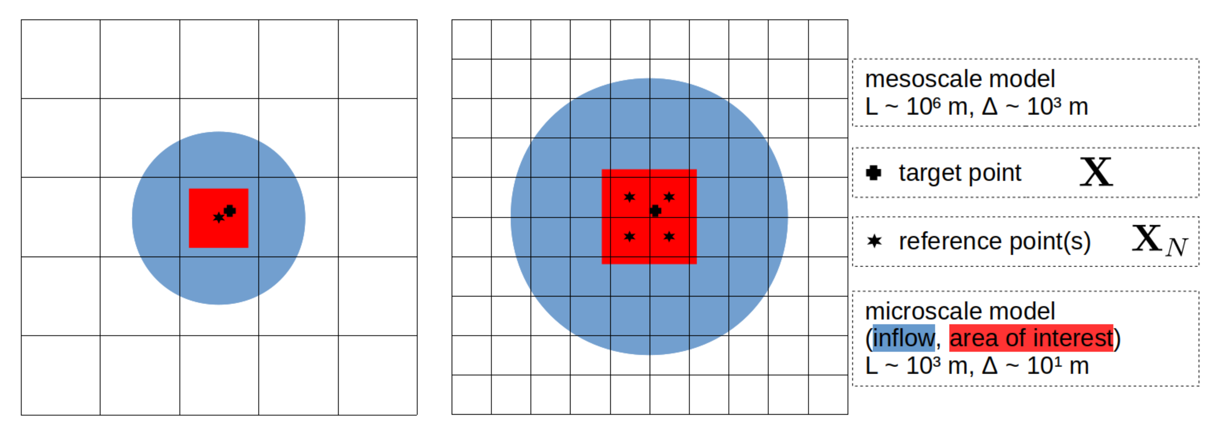
Figure 1 illustrates the general concept for the downscaling. The area of interest, i.e., the wind energy site, is highlighted in red and forms the inner part of the micro-scale domain, where the orography is sufficiently resolved to capture all relevant micro-scale effects. The blue area represents the inflow region for the micro-scale simulation. The simulated domain is usually some kilometers large with a resolution of around 30 m–150 m. The black grid lines represent the resolution of the meso-scale model, which has a relatively coarser grid typically in the order of a few kilometers in resolution and typically spans some hundred kilometers in its full extent (not shown). In the setup presented in the left part of the figure, the micro-scale model domain is completely within one meso-scale model grid cell. Thus, both models are coupled based on a single meso-scale grid point (hereafter referred to as single-point downscaling). So, the reference (meso-scale grid cell) and target points (e.g., a future possible turbine or met mast location for validation) fall into the same meso-scale grid cell. If the micro-scale model domain is larger than one meso-scale cell, as sketched in the right part of
Figure 1, the downscaling can be based on a number of meso-scale grid points that might lead to different results. Thus, a sophisticated combination is needed that is referred to as multi-point downscaling hereafter. Depending on the size and resolution of the models, a larger number of overlapping meso-scale grid points (reference points) is possible.
The general downscaling procedure itself is subdivided into the following steps:
Conduction of meso-scale simulations for the time period of interest or use of existing data.
Conduction of micro-scale simulations for multiple wind directions (and stability classes) for the site of interest. The simulation domain should be large enough to capture all site-relevant terrain.
Extraction of meso-scale data time-series at reference position(s) (overlapping with the micro-scale domain).
Extraction of (characteristic) wind profiles at reference and target position(s) from micro-scale model for each simulated state.
Downscaling of the meso-scale data to the micro-scale field at the reference position(s) (single-point downscaling-see
Section 2.2).
Optionally: Horizontally weighted interpolation of the downscaled wind fields from step 5. (multi-point downscaling-see
Section 2.3)
Optionally: For assessing the long-term wind climate: repeat steps 5–6 for the full wind climate and calculate relevant wind climate statistics (e.g., wind roses/histograms) at target positions.
Our approach is based on that proposed by Barcons et al. [
27], but the methods differ in some aspects. Firstly they use several overlapping micro-scale domains, while we use one large domain covering our site. This provides a more detailed representation of the local orography, as some orographic features can influence the flow dynamics downstream. Secondly, we extended the micro-scale model with a thermal solver, to account for stability in micro and meso-scale model. Thirdly, in our approach the reference height can be varied: The reference-point and target point are not necessarily at the same height. Another notable deviation is the calculation of characteristic profiles. With this we propose an improvement to the work from Barcons et al. [
27], as well as further showing the general validity of their proposed method with a proof of the concept at a benchmark site. For details of the method check the following sections.
2.2. Single-Point Downscaling
The single-point downscaling describes the scaling of the wind data from the high-resolution micro-scale wind field with the time dependent meso-scale data and can be noted as in Equation (
1):
where
N is the index for every reference position (
) and
is the respective time-dependent downscaled field.
are the steady-state pre-simulated micro-scale wind fields for different wind direction bins (
n) and
describes the scaling factor for the respective neighbouring wind field and is defined as Equation (
2):
The time dependency of the scaling arises from the time dependency of the meso-scale wind () and direction () data. The linear scaling is based on the wind direction difference between the (per direction bin) pre-calculated characteristic wind direction () and on the characteristic wind speed (). For example: We assume the micro-scale simulations are conducted in terms of 36 (equally spaced-at 0 to 350) wind direction bins and the meso-scale wind direction at the reference position is . We then analyze the characteristic wind speed at the reference position and find values like e.g., and , which would, in this case, come from the pre-calculated wind fields for 260 and 270 inflow direction that is modified by the flow in the micro-scale domain. Based on this we calculate the weighting factor and scale the meso-scale wind field for any target position and time step t.
Typically the meso-scale timeseries are only available for a limited number of height levels. Both micro-scale velocity profiles, as well as the meso-scale velocity timeseries, differ with height, therefore the scaling factors can thus only be calculated at these available height levels. The scaling can be applied to any target point within the micro-scale domain, regardless of height position. One option is to use a specific height level as reference or to linearly interpolate the scaling of multiple reference heights. We analyze this impact of the reference height in
Section 5.3.
2.3. Multi-Point Downscaling
In case of the situation that several meso-scale grid cells cover the extension of the micro-scale domain, not only the time dependent but also local horizontal meso-scale effects can be included into the downscaled field. This is done by repeating the scaling process (step 5) for all meso-scale reference points (
) that superpose with the micro-scale domain (in
Figure 1 these are exemplary four points). This is done using the following relation:
where
is the final downscaled wind field based on several meso-scale reference points,
is the downscaled wind field based on a single point Equation (
1) and
is an interpolation scheme, e.g., for the inverse distance weighting (e.g., [
29]):
where
is the inverse distance between the reference position (
) and the target position (
), with
N the reference point index and
p is the power factor, that could be a linear inverse distance weighting (IDW) with
or a squared inverse distance weighting (ISDW) with
. For
different interpolation schemes can be chosen. In the framework of this study we test the sensitivity of the resulting wind field to three different methods, a bi-linear method (BILIN) (e.g., [
30]), IDW and ISDW inverse distance weightings. For example, if the target position is located exactly in the middle, between the four reference positions the weighting factors
will all have the same value at this target position (
) and every single-point downscaled data is used equally. If the target position is located at the same location as our reference position (e.g.,
,
) only this downscaled field is relevant.
Equation (
3) describes a 4-dimensional problem in space and time. However, we do not produce this whole field for long time windows always, as typically only a limited number of certain target points is of interest and not the whole field. However, for situations with interesting or challenging atmospheric conditions (e.g., strong meso-scale shear or veer), it might be meaningful to analyze the downscaled velocity field at single time steps. We demonstrate this in
Section 5.1.
The standard site assessment procedure is to analyze long time scales to calculate average annual wind conditions and thus the projected annual energy production of the site, which would refer to step 7.
and
are then calculated for (a) specific target position(s)
only. The spatial interpolation
is time-independent and can be calculated in advance, this is also true for the micro-scale wind field database. Assuming existing meso-scale time series as e.g., from NEWA, wind time series for several years at the target points can be analyzed within minutes on a desktop computer. We demonstrate this application in
Section 5.2.
2.4. Thermal Stratification in the Downscaling Procedure
To include the impact of thermal stratification into the procedure, step 5 is modified such that the scaling takes into account the atmospheric stability. In this case a set of pre-calculated micro-scale wind fields, binned in terms of direction and stability (e.g., 10–36 classes of wind direction and 3–5 classes of atmospheric stability). The interpolation between the neighboring bins of direction is done as stated above, while the stability falls into pre-defined bins, based on the atmospheric stability in the meso-scale model. A pre-selection of the binning in terms of atmospheric stability and thus inflow conditions for the set of micro-scale simulations can be done based on the stability information from meso-scale data. Mathematically Equations (
1)–(
4) still apply, but the increment
n in micro-scale wind speed and direction refers not only to the different wind direction bins, but to the combination of wind direction bin and stratification bin.
2.5. Data Correction
In general, lower resolution model data such as meso-scale or global model data are known to be limited in terms of accuracy in comparison to mast data. Typically systematic errors are corrected in terms of a so-called measure-correlate-predict (MCP) method by a comparison of the model to mast data. A comprehensive review of MCP methods is given in [
31]. For that purpose, the linear regression between wind speed of mast measurements at the site and simulated results is performed Equation (
5). In case of pure meso-scale data, this is the wind speed at the closest meso-scale grid cell interpolated to target height from the heights available. The downscaled results are already extracted at the met mast location. The intercept parameter in the regression (not shown) is set to 0. This adds robustness to the correction. The general linear regression would lead to unphysical regressions in some cases. The regression gives this correlation:
is the wind speed of the simulated data (meso or downscaled),
and
are the locations of two different met masts on site,
and
the slopes of the resulting regression wind speed
. In opposition to the general MCP method, we apply the regression on the other met mast to get the corrected wind speed (
). If this is feasible, such a correction could be applied to any position within the domain.
2.6. Evaluation Metrics
For the analysis of the wind climate, we apply different evaluation metrics to compare the wind speeds of the meso-scale model, as well as downscaled and corrected results with measurements. These are the statistical bias (BIAS), root-mean-square error (RMSE) and the coefficient of determination (
R2), the latter as the square of the Pearson correlation coefficient (e.g., [
30]):
represents the meso-scale, downscaled or corrected wind speed and the measured wind speed. indicates averaging over all data points in the dataset. The BIAS can help to identify systematic errors. The R2 value represents the degree of spreading in our data, is not changed by the correction proposed above and gives a direct model feedback, even with systematic errors still present. The RMSE is a combination of both metrics and provides information about scatter as well as general BIAS.
5. Results and Discussion
The analysis of the results of the methodology introduced here consists of three parts: Firstly, in
Section 5.1, we identify, based on the meso-scale data, a single event where a strong local meso-scale horizontal wind direction change is present and therefore the potential benefit of the proposed method is prominent. Afterwards, in
Section 5.2 we apply the method on the full one-year wind time series to understand the improvement of the meso–micro downscaling on the representation of the wind climate. In the last part (
Section 5.3), we analyze the sensitivity of the long-term results to two additional aspects: the temporal resolution and the meso-scale height level used for scaling.
5.1. Single Event Analysis
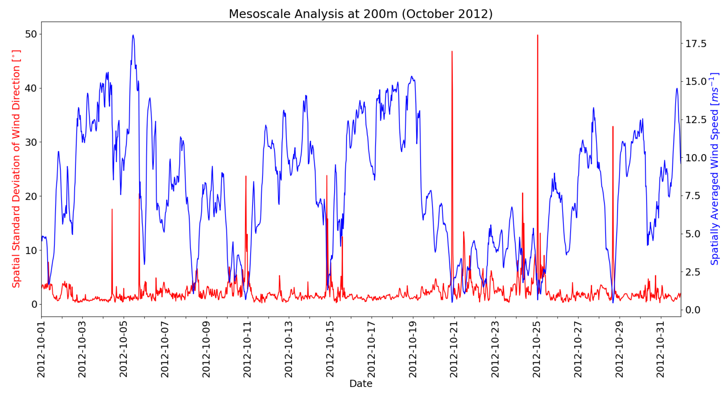
To identify situations with a strong regional wind direction change, we apply the simple methodology of calculating the spatial standard deviation of the meso-scale wind direction field around our target point and search for situations were this value is larger than within the NEWA dataset. An additional criterion is the wind speed. We look for wind speeds larger than 10 m/s, which is well above the cut-in wind speed for most wind turbines, and hence are most relevant for power production.
For this purpose, a grid of three by three grid cells around the Rödeser Berg site was extracted from NEWA, for which the innermost four cells overlap with the size of the micro-scale domain. Over these nine grid cells, the spatial standard deviation of the wind direction as well as the spatially averaged wind speed from the same grid cells are calculated for a full wind climate in 2012. October 2012 is plotted in
Figure 6. This time window includes a situation with both a strong change in wind direction together with a high wind speed on 5 October 2012 at 1800 UTC (see
Figure 6).
On this day, a fast moving secondary depression was moving from Great Britain across the Netherlands and Germany into the Baltic Sea area. During the afternoon the spatially averaged meso-scale wind speed at the site dropped from more than 15 ms
to below 5 ms
. At that time the cold front was moving over the site, with the typical strong change in wind direction (veering) and speed. Thus, this situation was selected for demonstration of the downscaling procedure of a single event. For that purpose, the downscaling methodology described in
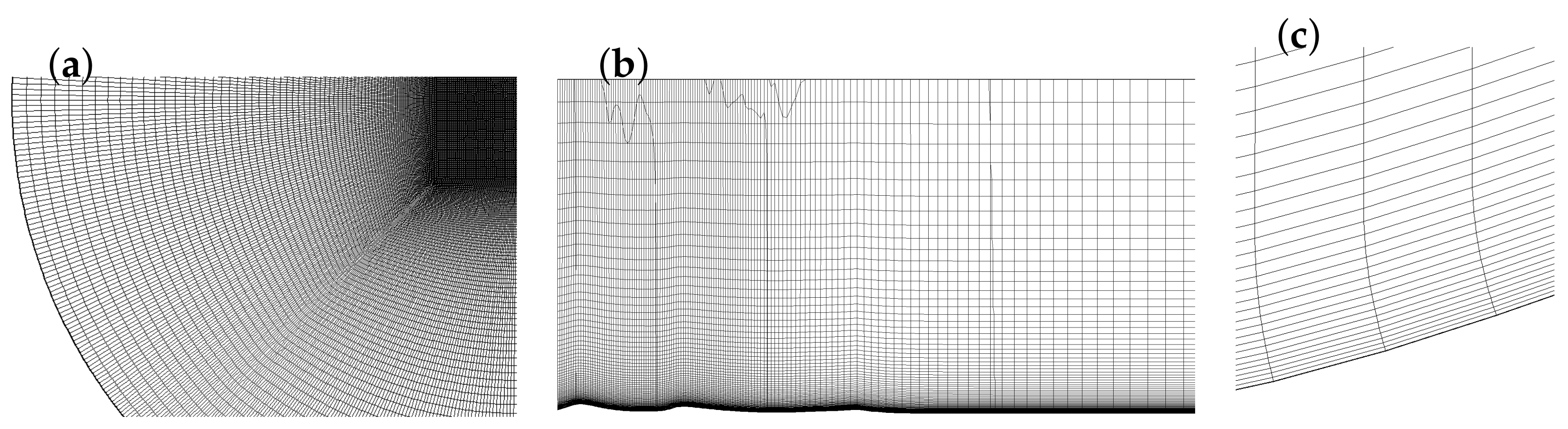
Section 2.1 was applied to the data set with different interpolation schemes to investigate their impact on the resulting downscaled wind field.
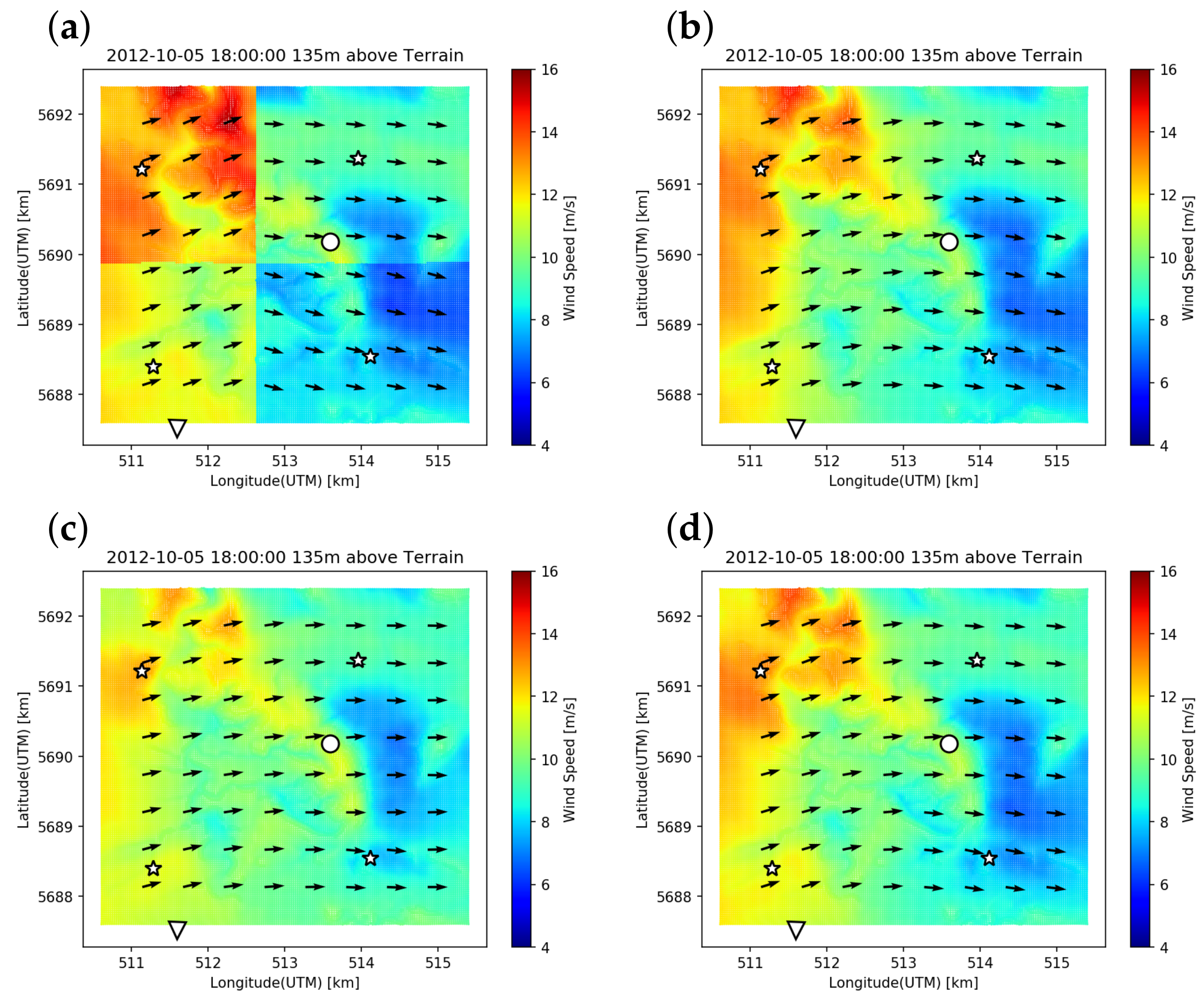
Figure 7 presents the downscaled wind field at hub height (135 m) from the same situation on 5 October 2012 at 18:00 UTC with the same meso-scale and micro-scale wind fields but different interpolation schemes for the multi-point assessment (step 6 in
Section 2.1). Without any interpolation (
Figure 7a) a strong unphysical discontinuity can be found to be related to the very different meso-scale wind speeds in the reference cells. The other panels represent different interpolation schemes: bilinear (BILIN-
Figure 7b), inverse-distance weighting (IDW-
Figure 7c) and inverse scaled distance weighting (ISDW
Figure 7d). The IDW (c) method can not be recommended, because outside of a very refined area around the reference grid point, all details are smoothed out. The ISDW (d) method shows good agreement with the BILIN (b) method, in particular in the center of the investigated wind field. At the edges, however, the smoothing effect is present, though less dominant compared to IDW.
This part of the analysis shows that situations of strong local shear and/or veer need a special treatment to be described satisfactorily. Furthermore, the interpolation adds a smoothing to the strong gradients provided by the meso-scale model. The presented downscaling mechanism provides an efficient analysis tool to include meso-scale effects into a micro-scale site assessment framework. However, despite this possible improvement in single situations, the ultimate test for such a method is the representation and improvement of the representation of the long-term wind climate that is typically needed in the site assessment procedure. We investigate this based on the one-year mast data set available from the two met masts at our test site.
5.2. Longterm Analysis
For the investigation of the impact of the presented meso–micro downscaling method on the (average) long-term wind conditions, the methodology (steps 1 through 7 in
Section 2.1) is repeated for a longer period in time (one year here). For proof of the methodology we use the data of the two met masts at the Rödeser Berg site. We will first analyze two different single-point downscaling schemes (
Section 5.2.1), afterwards analyze the impact of a multi-point downscaling (
Section 5.2.2) and the impact of taking atmospheric stratification into account (
Section 5.2.3).
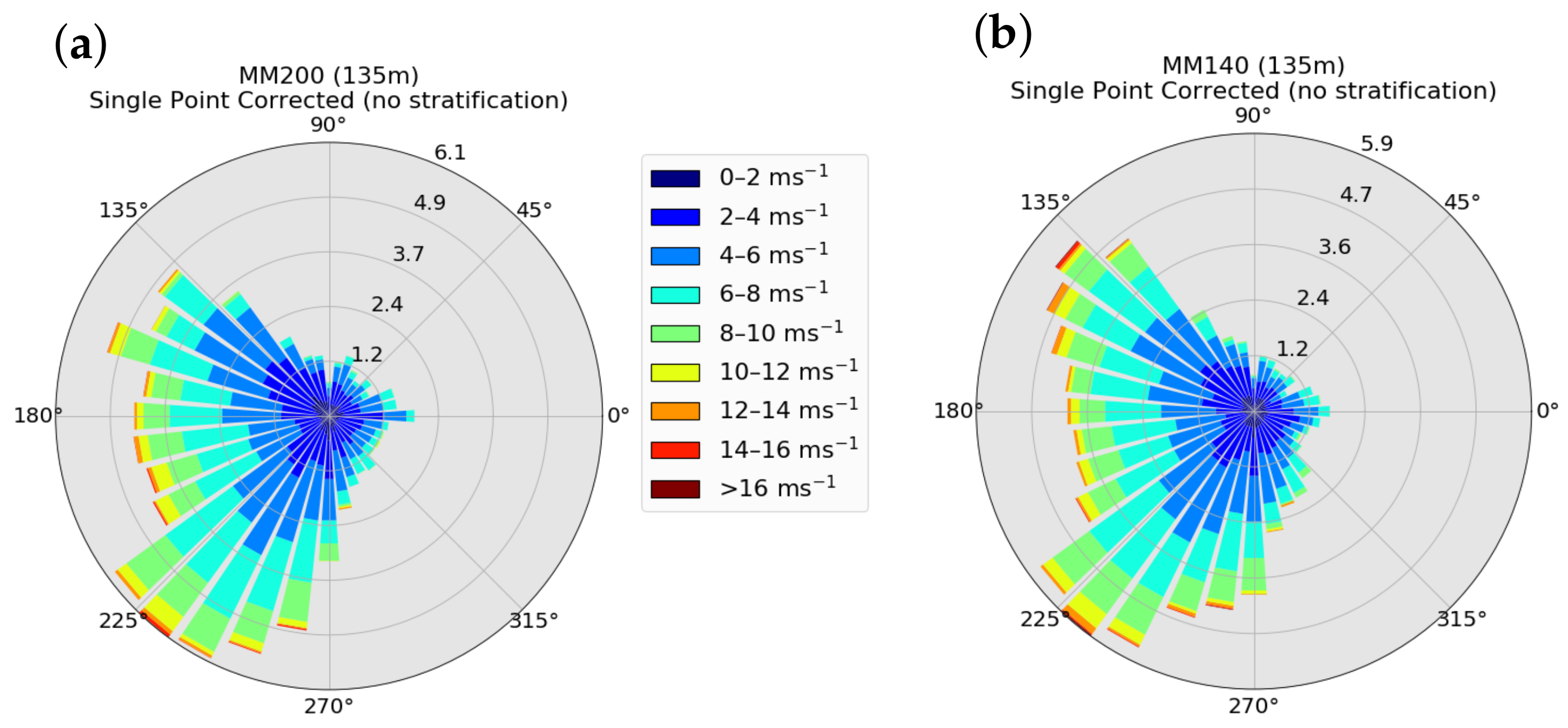
5.2.1. Single-Point Downscaling
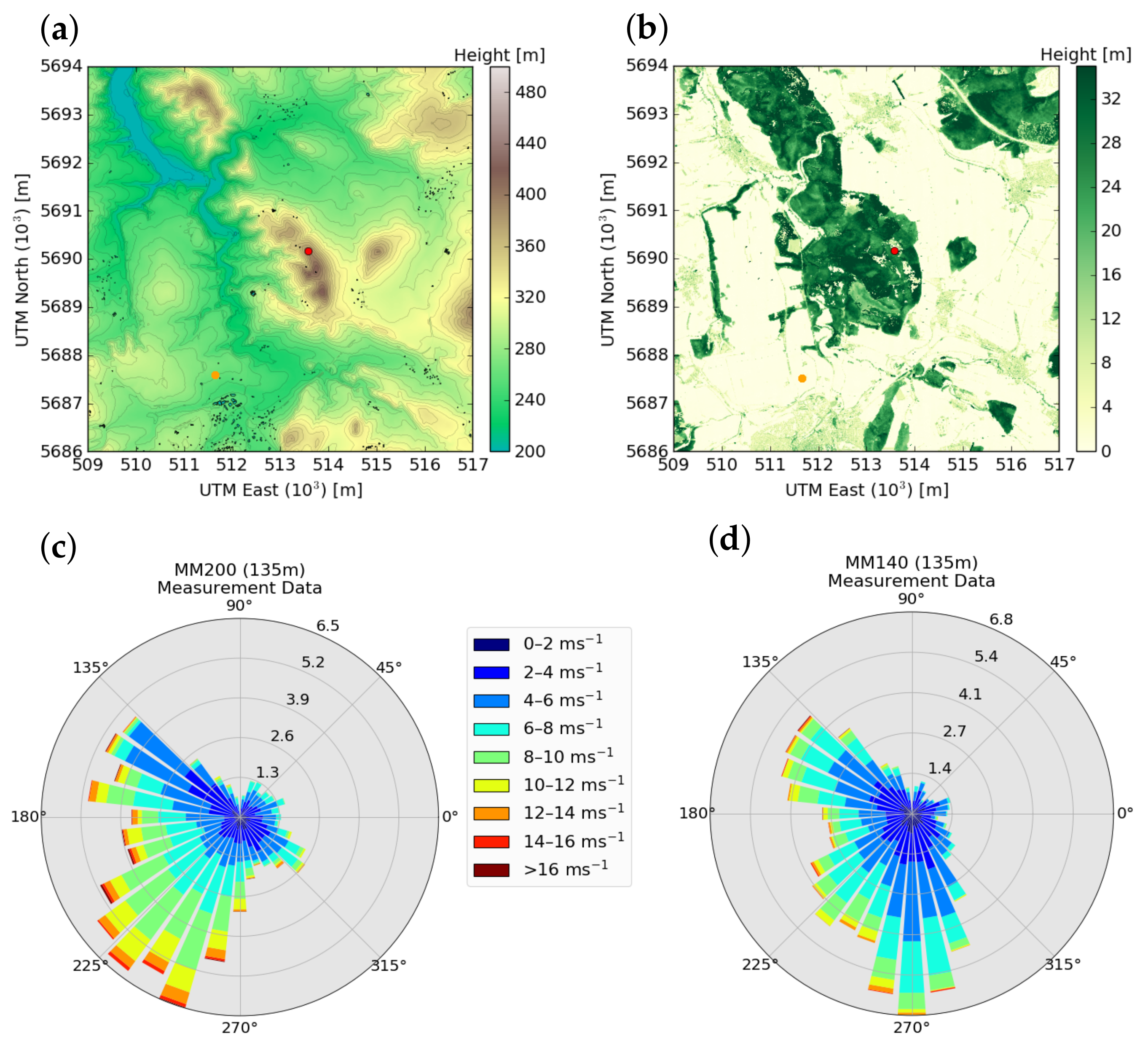
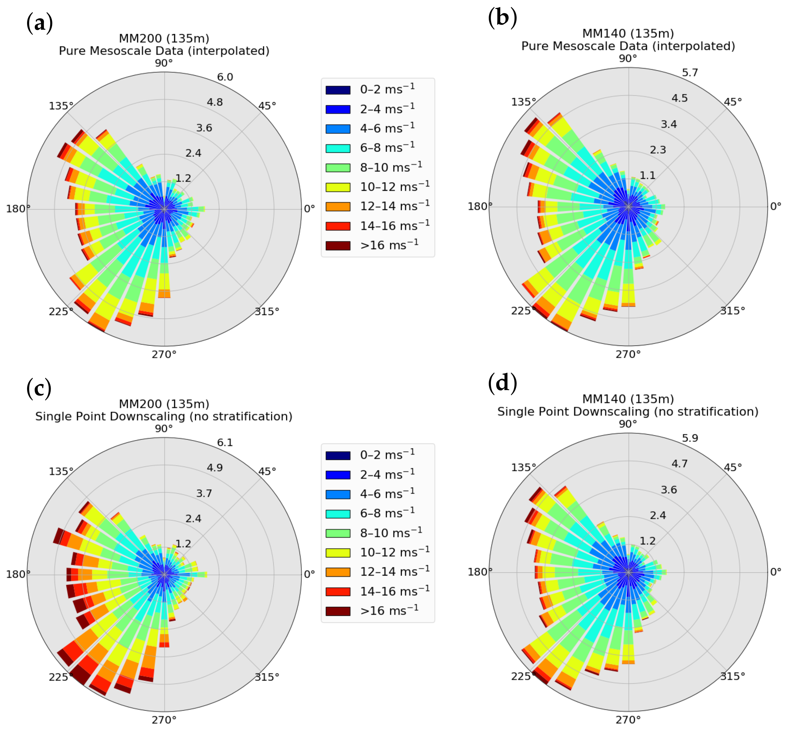
In the single-point downscaling method, we scale the micro-scale fields based on one reference-point from the meso-scale data only. In the setup for the Rödeser Berg case the extension of the micro-scale domain covers four grid points of the NEWA data. Each of the two metmasts (MM140, MM200) falls into another meso-scale grid cell, and hence has another meso-scale reference point as a basis for the downscaling.
Figure 8a,b show the wind roses (at the reference positions) based on non-downscaled pure meso-scale data, while the single-point downscaled wind roses are shown in
Figure 8c,d. In both cases, meso-scale data are linearly interpolated from the neighboring levels of the NEWA atlas (100 m and 150 m) to the measurement height (135 m) of the masts. To facilitate a comparison to the measurement data, a time period equivalent to those was selected from NEWA. The wind roses based on pure meso-scale data at the two mast locations are nearly identical, as the relevant meso-scale grid points are direct diagonal neighbors. The relatively coarse resolution of the meso-scale model (3 km here) is not capable of resolving the terrain adequately. This is in contrast to the meso–micro single-point downscaled wind roses in
Figure 8c,d and also the measurements in
Figure 2c,d in which an impact of the local terrain is prominent. In general, the downscaled wind roses (
Figure 8c,d) maintain the directional distribution of the meso-scale model to large extent with northwesterly winds being slightly more prominent at MM140 compared to MM200. The wind rose at MM200 (hill-top) further displays a strong speed-up effect. Both effects can also be identified in the measured wind roses (see
Figure 2c,d) though there still is a general overestimation at both mast locations in the downscaled wind roses. Furthermore, the downscaling cannot reproduce the southern wind sector, which is present in
Figure 2d. We identify two possible explanations: the Coriolis force might include a difference between the two target positions, due to the different heights above sea level. The micro-scale model applied in this study does not include the Coriolis force, and can thus not resolve this difference. Another reason is the orography around the area of interest. The metmast is located just north of the town of Wolfhagen and at the southern edge of our micro-scale domain. There is a north–south oriented mountain ridge in the southwest, which blocks southwesterly winds and leads to channeling southerly winds. However, this mountain ridge is not large enough to be covered by the meso-scale model and is also outside of our micro-scale model domain.
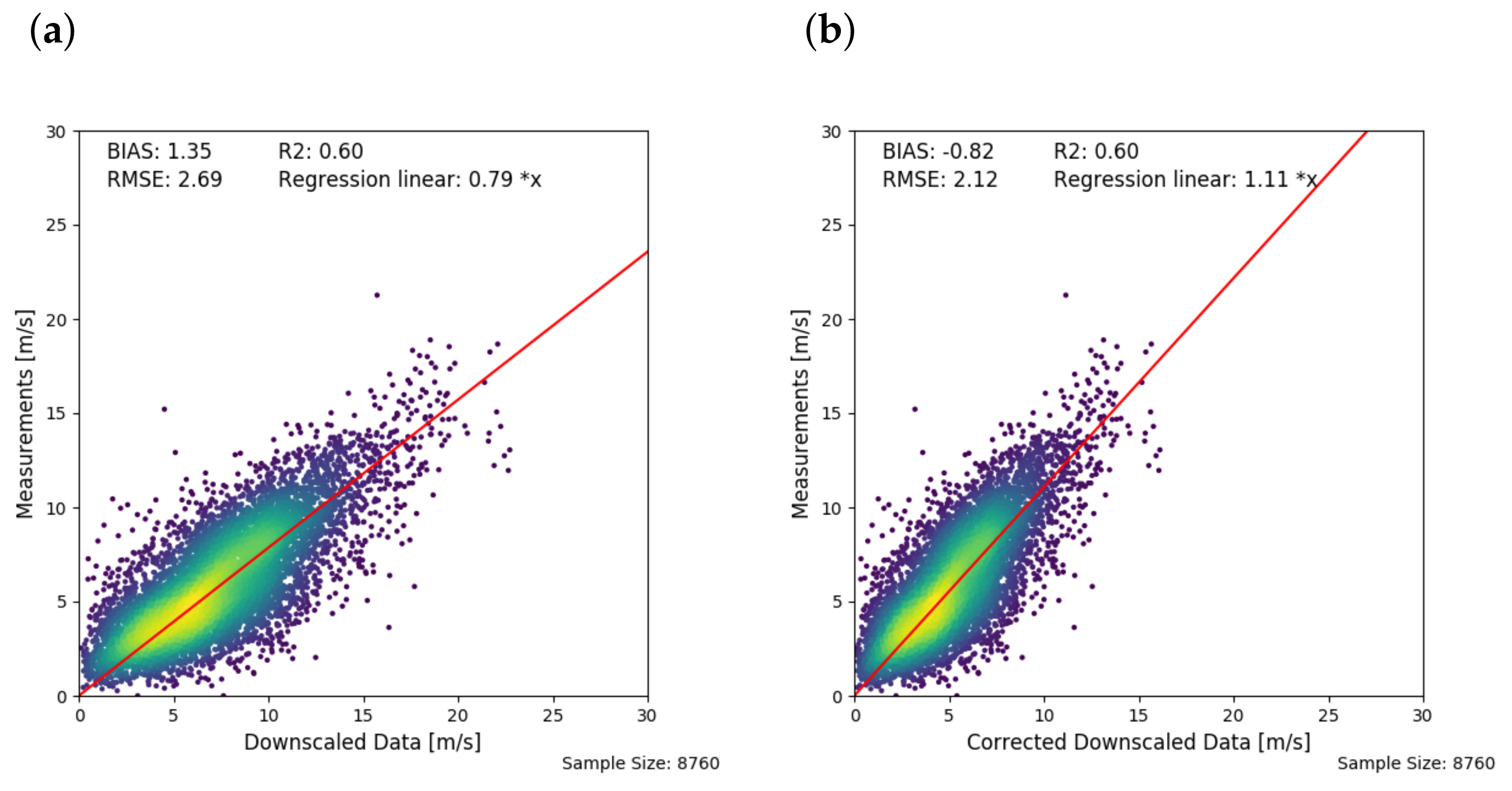
Nevertheless, the differences in wind speed and the shift in northwesterly directions, indicate a positive effect of the downscaling, when comparing it with the pure meso-scale data. In the next step we compare exemplarily the time series from the downscaling at the location of MM200 to the measurements. In
Figure 9a, a scatterplot showing the comparison between downscaled and measured wind speeds is presented. With a linear regression without intercept, we can identify a general overestimation of wind speeds in the downscaled data. A similar plot can be done for MM140, leading to a slightly different regression. For details of regression and evaluation metrics see
Section 2.5 and
Section 2.6, respectively.
As the site provides parallel measurements from two tall met masts, we can correct the downscaled data based on the linear regression from one mast and evaluate the improvement at the other one. Thus, we apply the data correction as described in
Section 2.5.
Figure 9b shows the data of
Figure 9a at MM200 after the correction with the linear regression based on mast MM140. In both scatter plots we can see different statistical values (for details check
Section 2.6. The
, or coefficient of determination, describes the spread of our scatter cloud which is not changed by the correction. BIAS and, as well as the root mean square error (RMSE) are reduced significantly by the correction. When comparing the resulting corrected and downscaled wind roses (
Figure 10a,b) with the downscaled non-corrected (
Figure 8c,d) and measured (
Figure 2c,d) ones, the improvement is standing out. Except for the southerly wind sector, the wind roses of MM140 already agree to a large extent. At MM200 the overall wind direction distribution matches to a good extent. Only the winds from the southwest show a larger disagreement. An underestimation is present.
We repeat this process for the meso-scale data and two different single point downscaling. For pure meso-scale we compare the metmast data to the nearest grid cell. These two grid cells are also the basis for the downscaling: Single Point 1 near MM140 and Single-Point 2 near MM200. The correction was always based on the data of the other mast. The evaluation metrics are shown in
Table 1. We can see, that without correction BIAS and RMSE of the pure meso-scale model are smaller compared to using a downscaling. When comparing the
values, it is almost constant at MM140 in all cases, while slightly better for the single point downscaling at MM200. When applying the correction, BIAS and RMSE become smaller in each setup, though to different extent. After correction, they are smallest for the downscaled data. This shows, that the general overestimation of the downscaled field is dominating the more detailed characterization of the downscaled field. Furthermore, after correction, we see that the downscaling itself leads to a better representation at the sites. At MM200, the
R2 value does change depending on the chosen reference point from the meso-scale data. Single point 2 is closest to the met mast and thus also yields the better coefficient of determination. In relative terms we can decrease the BIAS about
at MM200 and
at MM140 compared to meso-scale results (
and
for RMSE).
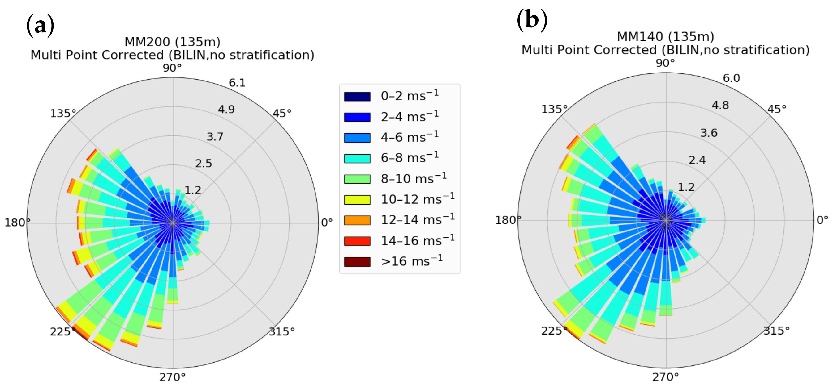
5.2.2. Multi-Point Downscaling
In the last section, we described the necessity of both the micro-meso downscaling and the data correction in combination, to increase the accuracy of the simulated data in comparison to the measurements. The next step is the comparison of a single-point downscaling to a downscaling based on multiple neighboring meso-scale grid points. Here, we use four neighboring meso-scale grid points covered by the extension of the meso-scale domain (as in
Figure 7).
The resulting wind roses after application of a BILIN interpolation scheme using neutral stratification in the micro-scale simulations only are given in
Figure 11. The wind speeds are slightly higher than in the single-point downscaling, however visually in the representation of the wind roses the differences are very small.
A statistical analysis of evaluation metrics for different multi-point interpolation schemes and between neutral and stratified cases (discussed in more detail in
Section 5.2.3) is given in
Table 2. The differences between the different interpolation schemes are small. In comparison to the single-point downscaling (
Table 1), we see an improvement in some of the statistical parameters. While the coefficient of determination cannot be increased, for MM200 it is even slightly smaller, the BIAS and RMSE are reduced. The combination of several single-point down-scalings to a multipoint down-scaling, does not only add robustness to the system, because the possibility of choosing a poor reference point is bypassed, but the data quality for the wind climate increases as well. Compared to pure meso-scale data we can decrease the BIAS about
at MM200 and
at MM140 compared to meso-scale results (
and
for RMSE). Values larger than
indicate an overcorrection.
The additional computational cost tradeoff between single and multi-point method is minimal as meso- and micro-scale data only needs to be computed once. The effort for the interpolation between different meso-scale grid cells in the post processing is negligible in comparison to the computing time of the meso and micro-scale simulations itself.
5.2.3. Multi-Point-Downscaling with Thermal Stratification
In this section, we discuss the results of the impact of the consideration of stratification in the downscaling framework. The analysis is done in analogy to the previous section where a focus is given to the final statistics of the wind climate. Based on the stratification at the reference position, we select the representative neutral, convective or stable micro-scale simulation for the downscaling (compare
Section 2.4 and
Section 4.2).
Table 2 provides a comparison of several statistical quantities obtained for the downscaling with thermal stratification with those obtained for the downscaling where always neutral stratification is assumed. For both met masts no clear improvement of the results of the downscaling can be seen when stratification is taken into account. For MM200 the BIAS is slightly smaller compared to neutral, but the
R2 value is smaller as well. For MM140 the BIAS was already very close to 0. The value got slightly worse, but is still small. In analogy to the previous sections, we can decrease the BIAS about
at MM200 and
at MM140 compared to meso-scale results (
and
for RMSE).
Using the given data, we compare six different setups in
Table 3. The first three assume again a uniform stability throughout the time series. On one hand, the already analyzed, purely neutral downscaling, on the other hand, convective and stable stratification (
m and
m). Thus, a single micro-scale field (in regard to stratification) is used no matter the actual stratification. In the lower part of
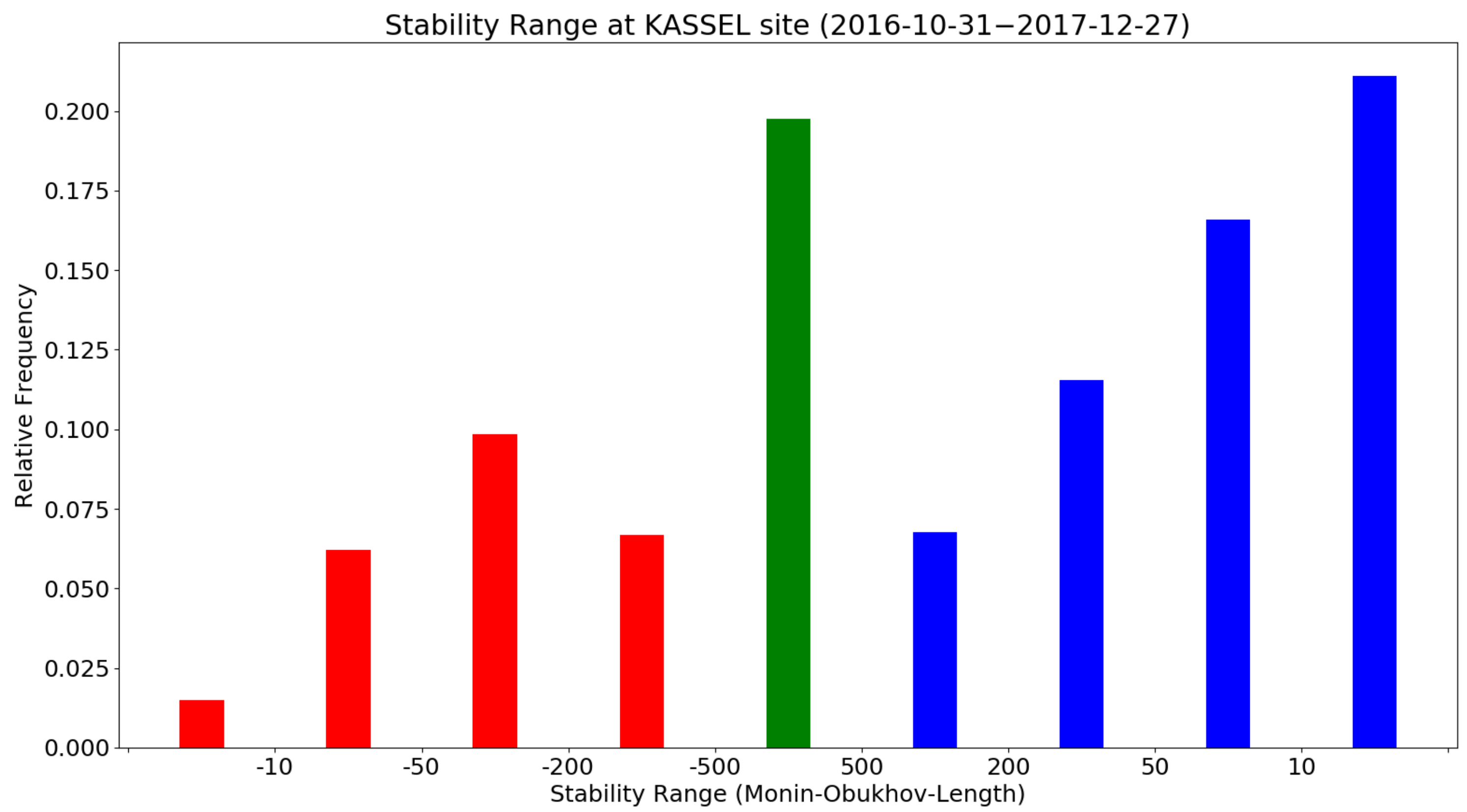
Table 3 we evaluate the performance of the downscaling separately for the actual stratification given by the meso-scale data. The share of the three stratification classes are given in
Figure 4. When using the full time series (first three rows of
Table 3), RMSE and
R2 are nearly independent of the assumed stability, only the BIAS changes. At MM200 the convective stratification shows the largest BIAS, while it is largest at MM140 for stable stratification. This is connected to the locations of the met mast, MM200 at the hill-top and MM140 in the valley. The stronger vertical wind speed gradient in stable stratification better represents the shear at the hill-top. Overall, the downscaling assuming stable stratification leads to more representative results than using a neutrally stratified micro-scale field. This is consistent with the prevailing stable stratification of the wind climate at the site. When applying the downscaling to those timesteps with a specific stratification only, we find strong differences between neutral and non-neutral setups. For the neutral setups, BIAS and
R2 values are very close to the original neutral setup. The RMSE is smaller in stratified flows at both met mast locations. The RMSE is directly connected to the average wind speed. Large wind speeds produce mixing in the atmosphere and hence often neutrally stratified flows. For the same reason, the RMSE is smaller in convective and stably stratified situations. Though the BIAS in both stratified cases is reasonable, the
R2 dropped to 0.56 and 0.50. This indicates that a large spread in the data is still present, and the representation of stability is not sufficient.
5.3. Sensitivity on Reference Height and Temporal Resolution
In order to analyze the impact of the reference height and temporal resolution of the meso-scale data on the results of the multipoint downscaling approach, we carried out a sensitivity study. For this we applied the multi-point scheme with BILIN interpolation and included stratification. We compared only those results that were obtained after the correction with measurements had been carried out.
First of all, we compare different reference heights and their influence on the long-term analysis. Note that the target height is always 135 m above the surface, only the reference height from the meso-scale model changes. We analyze the impact of the reference height on the downscaling performance. We included five fixed single reference heights (50 m, 100 m, 150 m, 250 m, 500 m) and one interpolation. The latter combines the downscaled results from the two closest reference heights (100 m and 150 m), vertically interpolated according to the distance from the target height.
Table 4 shows a nuanced picture for the two metmasts. At MM140 the BIAS is smaller for higher reference heights, while for both masts the
R2 value is largest with a reference height of 50 m. Overall however the statistics are better, the closer the reference height is to the target height. The interpolation of different reference heights, includes the turning of the wind (due to the Coriolis force) indirectly into the system. As the Coriolis force is not accounted for by the micro-scale model (compare
Section 4.2), we decided to use the interpolation of the closest reference height throughout the paper. While all results presented in the previous sections were based on 1 h mean values from the meso-scale model, we did also study the impact of applying other temporal averages on the downscaling. The impact of the different means on the evaluation metrics is shown in
Table 5. The BIAS is nearly constant, but with longer temporal averaging
increases and RMSE decreases. The impact of smaller averaging periods could not be analyzed, as the meso-scale data was only available every 30 min. With longer averaging, many temporal characteristics are lost as well. Therefore we decided to use 1 h averages.
6. Conclusions
In this study, we described and evaluated a multi-point meso–micro downscaling framework. We demonstrated that the methodology can be used for challenging single situations to understand the dynamic of certain synoptic situations with strong horizontal meso-scale direction changes at a given site and also showed that it improves the representation of the wind climate compared to meso-scale model results. The methodology is a post-processing method that efficiently combines and interpolates between meso-scale and micro-scale wind fields for a given site and is thus in principle independent of the meso- and micro-scale models. The analysis of a single event showed that in situations with a strong meso-scale shear or veer, a downscaling based on multiple meso-scale grid points is crucial, to include this meso-scale changes into the micro-scale domain. We further tested the sensitivity of different parameters for the downscaling, e.g., the interpolation scheme to interpolate between horizontal meso-scale grid points.
By an analysis of parallel measurements at two met masts in the complex terrain of about one year, we analyze the long-term impact of the downscaling. This was done systematically by comparing pure meso-scale data over downscaling on a single-point to multi-point downscaling and included a correction of the systematic errors of the model data by one mast and an evaluation at the other mast. In respect to the pure meso-scale results the BIAS can be reduced up to
with a single point downscaling and up to
(overcorrection of
) with a multipoint downscaling. Similarly the RMSE decreases, though to a lesser extent. The neutral multipoint downscaling is similar to [
27], and hence we can confirm the validity of the general approach based on a well-studied benchmark site. The new introduction of stratification in the micro-scale model comes up with a differentiated picture: an improvement was not shown in all cases. A more detailed analysis on stratification in micro-scale simulations is necessary. For example more stability classes might be required, or the stability needs to be scaled. Furthermore, the stratification information in meso-scale models is crucial in thermal meso–micro setups. Improvements in that field, directly reflect within the downscaling.
Overall we see the following advantages of the presented methodology:
Downscaling in general combines strengths of micro and meso-scale simulations.
The multi-point downscaling is particularly useful in complex flow conditions
A downscaling is necessary to resolve local orography, in comparison to pure meso-scale simulations
The long-term multi-point downscaling improves the results compared to pure meso-scale results and makes it more robust than a single-point downscaling.
The significance of a multi-point downscaling methodology will improve with increasing computational power
For the generation of meaningful results, it is important that the micro-scale model domain is large enough, covers all target points (e.g., met masts) and several meso-scale grid points. It is further important to include all significant orographic features (e.g., mountain ridges) and our analysis indicates that large domain sizes are presumably better to cover all features, than several overlapping domains. However, as the downscaling is a statistical one, a defined number of simulations need to be carried out only, in contrast to a dynamical downscaling that can be very costly. In the future, further research on the impact of stratification and its inclusion in the downscaling procedure could be done. This would for instance also include a sensitivity study towards the number of stratification classes possibly also for a number of sites. Lastly, the impact of the reference height needs to be reevaluated for models including the coriolis force and hence the Ekman spiral. The combination of atmospheric stratification with the coriolis force is an ongoing challenge in micro-scale modeling.
In this study, we have investigated a time frame of one year only as parallel measurement data at two masts were available. However, the downscaling could also be based on a full (e.g., 30 year) wind climate and e.g., use the full meso-scale dataset of NEWA. Thus, a down-scaled wind climate for the entire lifetime of a wind farm would be possible. In the future, one could also replace the steady-state micro-scale model with the average wind fields from LES, which could especially in very complex terrain lead to better results.


 ,
, 


