Abstract
The Chinese government has launched a guideline for carbon emissions up to the peak (CEUP) in the 2030 target. The electric power sector has to make its own contributions to the national CO2 emissions mitigation target. In this study, a patron–client interactive optimized (PCIO) model is proposed to investigate the regional energy–water–carbon nexus optimization under the policy background of the CEUP target. Inner Mongolia, the largest energy base in China, which is also facing the prominent contradiction including the energy production and serious environmental problems, is chosen as a case study. Multiple uncertainties, including the fuel price uncertainty and output of the wind and solar power, are considered to make the optimization process more realistic. Results show that coal-fired power will gradually be substituted by the gas, wind, and solar power in Inner Mongolia to reach the CEUP target. The CO2 capture and storage technology and air-cooling systems will play important roles, especially under the strict water policy scenario. However, the achievement of the CEUP and water-saving target will be at the expense of high system costs. The PCIO model makes it possible for the decision-maker to make flexible strategies to balance the CEUP target and saving system costs. The results have demonstrated the validity of the PCIO model in addressing the hierarchical programming problems.
1. Introduction
China has announced to the world that in 2030, carbon emissions will reach their peak so that it can make effective contributions to the global CO2 emissions target. This target is China’s national pledge to reduce carbon emissions, which will further help China switch the extensive economy mode to the low-carbon economy mode. To achieve this target, all sectors should assume responsibility and undertake the corresponding systematic reduction in CO2 emissions. The electric power industry is the major CO2 emissions contributor in China, which is responsible for 44% of the total CO2 emissions in 2015 [1]. This amount is 1.5 times higher than that in the United States (US) and 2.5 times higher than that in European Union (EU), while China’s electricity consumption per capita only accounts for a quarter of that in the US and one-half of that in EU [2]. The electric power industry in China needs to make great efforts to optimize its structure further and improve the energy efficiency so that the CO2 emissions up to the peak (CEUP) target could be achieved as scheduled.
Thermal power, especially coal-fired power, is still in the dominant position in China’s electric power system (EPS). In 2017, the installed generating capacity rose by 7.6% to over 1770 GW; among them, over 60% was thermal power [3]. Although the Chinese government has promulgated a few enforced policies to remove inefficient generation units, some studies have pointed out that there would be little CO2 reduction and large reduction fees during 2015–2020, and a lock-in effect during 2015–2030 [4]. To guarantee the CEUP target will be achieved by 2030, there are some key strategies: First, thermal power should further promote energy efficiency and shut down the outdated production facilities [5]. Second, optimize the power supply structure further, and expand the application scope of the renewable energy, such as wind and solar power, instead of the new installation of thermal power [6]. Third, it is suggested that the CO2 capture and storage technology (CCS) have vigorous development to assist the CO2 emissions mitigation target, for this technology can safely capture and store about 90% of the CO2, which is a key measure for the sustainable use of large-scale fossil fuels [7]. However, the high cost of CCS technology poses the main barrier to its widespread application as the CO2 control strategy. So not only for the power structure optimization but also for the application of CCS to achieve the CO2 mitigation target in 2030, scientific planning is important and essential. In the meanwhile, as the thermal power plants in China are mainly distributed in arid and semi-arid regions, the water withdrawals of the thermal power plants have become a significant issue. The regional contradiction between energy supply and water resource consumption is prominent, especially in recent decades [8]. In this way, investigating a scientific framework, including the regional electric power structure adjustment, CO2 emission mitigation, and water withdrawal saving optimization, which is called the energy–water–carbon nexus optimization under the 2030 carbon emission up to the peak target, is rather important.
The nexus studies have gradually become the research hotspot in recent years. Many studies focused on the energy–carbon nexus or the energy–water nexus. Gao et al. [9] first uncovered the CO2 emission trajectory of China’s pharmaceutical industry and then identified the key driving forces of its emission growth. Anwar et al. [10] investigated the tourism and natural resources in energy–growth–CO2 emission nexus for 51 “Belt and Road Initiative (BRI) countries” over 1990–2016. Liu et al. [11] explored the energy saving/water saving of different policies in Beijing in the future and its nexus effect based on 26 scenarios. Zhai et al. [12] investigated the three main cereals (i.e., wheat, maize, and rice), their potential environmental footprint and spatial variation, and key factors in 2017 in China. However, studies on the energy–water–carbon nexus, especially the nexus studies in the EPS, are still limited. Most existing energy–water–carbon nexus studies focused on the food supply security [13], or the ecological network system [14]. Although Liu et al. [15] and Wang et al. [16] studied on the regional EPS planning concerning the energy–water–emission nexus, as their planning target just served the regional electric power structure adjustment strategy, they could not give effective guidelines and policy suggestions for the CEUP target of China. In this way, investigating available ways for the regional energy–water–carbon nexus optimization under the policy background of the CEUP target is important and urgent, for they can provide scientific guidance for the path of realizing the CEUP target in China.
Most studies carried out on the regional nexus studies were based on the optimized methods. Piao et al. [17] built a single-objective stochastic simulation–optimization model to deal with the energy–emissions problems in Shanghai’s power sector, including the energy supply uncertainty. Majid et al. [18] proposed a multi-objective mixed-integer linear programming model to investigate the energy–water nexus in building a system. However, the single objective cannot effectively deal with problems with conflicting objectives in the nexus studies. Although the multi-objective method has more than one objective to represent different targets simultaneously, each objective is on the same level. It also has difficulties in dealing with problems with the hierarchical structure. Different from the multi-objective programming method, bi-level programming theory has the advantages of being able to tackle interactive decision-making units within a predominantly hierarchical structure [19], which can effectively deal with dual conflicting objectives in the regional energy–water–carbon nexus study. This paper proposes a patron–client interactive optimized (PCIO) model based on the bi-level programming to explore the regional energy–water–carbon nexus optimization under the background of the CEUP target, and investigates the best tradeoffs in the regional EPS in China. Multiple uncertainties, including the fuel price and the output of the wind and solar, are taken into consideration in this study. Inner Mongolia, the largest energy base in China, is chosen as a case study to verify the availability and efficiency of the proposed PCIO model.
2. Methodology
2.1. The Algorithm of PCIO Model
Bi-level programming (BLP) is a special kind of statical Stackelberg game with two decision-makers at two different levels [8], a case of two-person, non-zero-sum, and full information game. It has the superiority in tackling problems with a hierarchical framework and helps to get a compromised solution between two levels [20]. The patron–client interactive optimized (PCIO) model was formulated based on the framework of the BLP model. The patron (upper) level of the PCIO model is to maximize the renewable power penetration ratio in Inner Mongolia; The client (lower) level of the model is to minimize the system cost. A fuzzy satisfaction degree method [21] is introduced to solve the PCIO model. As the values of the decision variables and function of the patron (client) level will be the in-put parameters of the client (patron) level to build the triangle membership function, both levels will exert influences on the other level. Coupled with the carbon emission and water withdrawals restraints in two level, the proposed PCIO model is applied to optimize the energy-water-emissions nexus in Inner Mongolia. The flow chart of algorithm is shown in Figure 1.
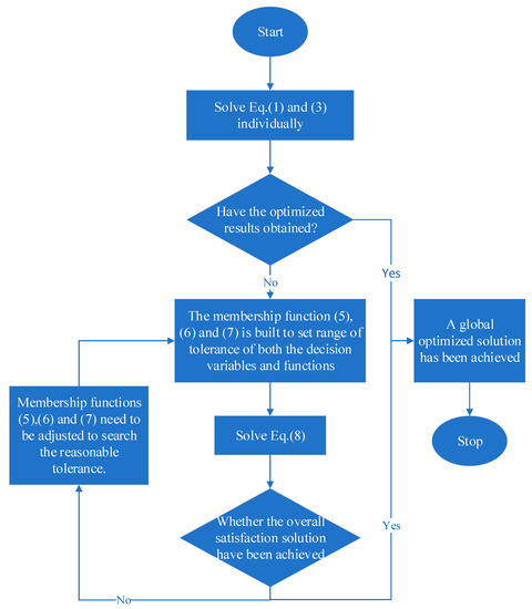
Figure 1.
The flow chart of the PCIO model.
The algorithm of the fuzzy satisfaction degree method for the PCIO model is shown below:
The upper-level objective and its constraints:
The lower-level objective and its constraints:
where (,,) is the optimized solution of Equation (1). (,,) is the optimized solution of Equation (3). is the maximum tolerances around . / is the result when the optimized decision variables of Equation (3)/Equation (1) is put into Equation (1)/Equation (3). , and are three membership functions, which is built to restrain the minimum acceptable degrees of satisfaction . If the upper-level decision maker is satisfied with the solution in [22], a satisfactory solution is reached. Otherwise, new membership functions for the decision variables and the objective function will be generated and the computation process is repeated until a satisfactory solution is reached.
2.2. The PCIO Model
The functions, decision variables and parameters are presented in Table 1. The detailed information of each variable and parameter are shown close to the PCIO model.

Table 1.
The decision variables and parameters of the PCIO model.
2.2.1. Patron Objective
The patron-level objective emphasizes the maximization of renewable power penetration during the planning periods in Inner Mongolia, which is stated as:
where denotes renewable power penetration in the electric power system. denotes the amount of electricity generated by power conversion technology j. j = 1, 2, 3, and 4 represent coal-fired power, gas-fired power, wind power, and photovoltaic power, respectively. denotes the pre-regulated installed capacity of the electricity schemes (MW). denotes the binary variables to identify whether a capacity expansion action of power conversion technology j should be executed. denotes the expansion capacity for conversion technology j (MW). is the utilization hours of conversion technology j (hour).
Considering the relationship between the path of achieving the carbon emissions peak and the harmonious development of the local economy, constraints of the environment–economy performances are taken into account at the patron level:
Coordinated constraints for the environment–economy performances [23]:
where and denote the optimal and the minimum regional harmonious development index, respectively, in which the predetermined value of was 0.8 in this model [23]. Details about the synergetic relationship for the environmental and economic performances of the systems are presented as follows:
Membership function denotes the coordinated degree between electricity supply and demand:
where is defined as the ratio of total power generation to power generation amount in 2005, which is expressed as:
where denotes the power generation amount of Inner Mongolia in 2005.
Membership function denotes the coordination degree between regional economic performance and carbon emissions level, stated as:
where is the ratio of carbon emissions to regional economic performance, presented as
where and denote the reference coefficients for the carbon emissions and the economic cost of the systems. In this study, the carbon emissions and the economic cost of Inner Mongolia’s electric power system in 2005 were chosen as the reference coefficients, respectively. and denote the actual value of carbon emissions and system cost in different years.
Constraints for total CO2-emissions are as follows:
where denotes CO2-emissions rate by power conversion technology j in period t (tonne/MWh), is the CO2 reduction efficiency through the CCS technology in period k (%). is the proportion of the thermal power plants with the CCS devices (%). is the CO2 emission limit from the thermal power plants in period k. is the excess CO2 generated from power conversion technology j in period k (103 t)
2.2.2. Client Objective
The system cost contains seven sectors, including the purchasing cost for energy and water resources, the cost for capacity expansion and electricity transmission, the cost for CO2 emissions mitigation, etc.
where (1) the cost for purchasing energy and water withdrawals:
(2) the operating cost for power generation:
(3) the penalty for power shortage:
(4) the cost for capacity expansion:
(5) the revenue for electricity transmission:
(6) the cost for CO2 capture and storage:
(7) the penalty for excess CO2 emissions:
where i denotes the type of energy, i = 1, 2 for coal and natural gas, respectively. denotes the amount of energy supply from source i in period t (PJ), is the price of coal and natural gas in period t (106 RMB ¥/PJ). denotes the cost for water in period k (106 RMB ¥/tonne), is the number of water withdrawals in period t under the water supply policy scenario p (tonnes). p denotes the water supply policy (flexible and strict). denotes the water withdrawal factor of different power generating technologies (m3/MWh). k is the type of cooling technologies, k=1,2,3 denotes the cycling cooling, one-through, and air-cooling system, respectively. is the kth proportion of cooling technologies (%). (2) denotes the operating cost for power conversion technology j (106 RMB¥/PJ). (3) denotes the probability of different electricity demand-level h (%). is penalty cost for power shortage (103 RMB/MWh). is the amount of power importing from other regions when the power shortage occurs (MWh). (4) denotes the expansion cost for conversion technology j in period t (103 RMB¥/MW). (5) denotes the revenue per unit of electric power transmitted to other regions. denotes the transmission ratio of total power generation (%). (6) is the construction investment for carbon capture and storage (CCS) technology (RMB/MW). is the benchmark technology cost for CCS technology (RMB/MWh). denotes the financial subsidy in period t. (7) denotes the operating cost for excess CO2 released from power conversion technology j in period t (106 RMB¥/tonne).
The constraints for resource availability:
and denote total energy resource supply level to generate electricity in period t (tonne) and total water resource supply level to generate electricity in period t (tonne), respectively.
The constraints for energy supply and electricity generation:
denotes the unit of electricity generation per unit of energy carrier for energy i (GWh/PJ).
The constraints for power demand-supply balance:
denotes power loss for power conversion technology j in each planning period, denotes the electricity demand in Inner Mongolia in each period (103 GWh).
The constraints for realizing CO2 emissions peak:
denotes the CO2 emissions of Inner Mongolia from the electricity industry in 2005 (103 tonne).
The mass balance for water withdrawals:
denotes the water withdrawals per unit of electricity generation (tonne/GWh), is the total water resource supplies underwater withdrawal policy p (tonne).
The constraints for expansion capital:
denotes the expansion cost for conversion technology j in period t (103 RMB¥/GW), denotes the power plants expansion fees in period t (106 RMB ¥).
The constraints for the interval-integer variables:
2.3. Uncertainty Analysis
2.3.1. Measuring the Fuel Price
The fuel price here includes two kinds of fuels, coal and natural gas. We assumed that both of their prices followed the Geometric Brownian Motion [24]:
where denotes the fuel prices; is the drift parameters; is the variance parameter, and denotes the independent increments of the Wiener process.
The discrete approximation to (1) is as follows:
where is a random variable, and .
2.3.2. Measuring the Output of Wind Power and PV
(1) The output of wind power
It is well established that wind speed distribution follows the Weibull probability density function (PDF) [25,26]. The probability of wind speed v (m/s) following Weibull PDF with shape factor (k) and scale factor (c) is given by:
The mean value of Weibull distribution is defined as:
where gramma function is described as:
In this study, the empirical values of the Weibull shape (k) and scale parameter (c) in three planning periods are different. In this way, the wind power output in three periods can be simulated. The function of wind speed (v) is described as:
where , , and are the cut-in, rated, and cut-out wind speeds of the turbine, respectively. is the rated output power of the wind turbine. The various speed values were = 3 m/s, = 16 m/s, and = 25 m/s. Figure 2 was obtained through Monte Carlo simulation by the sample size of 10000.
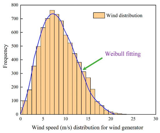
Figure 2.
The distribution of wind speed through the Monte Carlo simulation.
(2) The output of solar power
The output of the solar power depends on the solar irradiance (G), which follows the lognormal PDF [27]. The probability of solar irradiance (G) following lognormal PDF with mean and standard deviation is:
In this paper, and G = 483 W/m2 were based on [28].
The mean of the lognormal distribution is defined as:
The solar irradiance (G) to energy conversion for solar PV is given by [29]
where is the solar irradiance in a standard environmental set as 800 W/m2. Rc is a certain irradiance point set as 120 W/m2. is the rated output power of the solar PV unit. Similarly, Figure 3 was obtained through Monte Carlo simulation by the sample size of 10,000 [28].
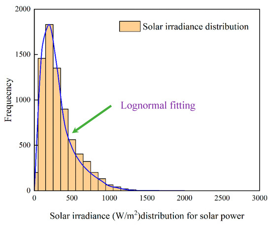
Figure 3.
Solar irradiance (W/m2) level through the Monte Carlo simulation.
3. Scenario Setting
This study mainly concerned three key time nodes in the path of achieving the carbon peak of China during the energy–water–carbon nexus optimization in Inner Mongolia, including 2021, 2025, and 2030. Different non-renewable and renewable technologies were taken into consideration to meet not only the electric power demand and the CO2 emissions mitigation target but also the water conservation goals. As the Chinese government announced that by 2020, China’s CO2 emissions intensity targets would fall by 40%~45% based on 2005’s level, by 2030, the CO2 emissions intensity targets would fall by 60%~65% based on 2005’s level, and the carbon emissions peak of China would be achieved. In this study, we assumed that the upper bound of these targets could be achieved as scheduled. Three CO2 emissions mitigation scenarios were set based on this official statement in these planning periods. The CO2 emissions’ intensity in 2005 was the baseline. For example, GHG intensity will decrease by 45% of that in 2005 in period t = 1 (2021), and it will be 60% and 65% of the baseline in the next two periods, respectively. Meanwhile, three different electricity demand levels (low, medium, and high) with different occurrence probability were designed to cover different electricity supply likelihoods. As Inner Mongolia is located in a typical semi-arid region with drought-stressed water resources, two possible water conservation policy scenarios were taken into account, including three main cooling technologies in each scenario. The mix of these scenarios will help investigate the energy–water–carbon nexus during the achievement of the carbon emissions peak path in 2030. The detailed, flexible, and strict data were based on the national water intake standard: Water Quota Part I: Thermal Power (GB/T18916) [30] and Water Saving Enterprise: Thermal Power Industry (GB/T26925-2011) [31], which is shown in Table 2. The pre-regulated installation capacity of each power technology is presented in Table 3. The key parameters of the PCIO model are shown in Table 4.
Table 2.
The water withdrawal factor of different technologies under two scenarios (m3/MWh).
Table 3.
The pre-regulated installation capacity in Inner Mongolia (MW) [32].
Table 4.
Economic and technological data for different power plants.
4. Result and Discussion
4.1. The Uncertainty Simulation in Different Periods
(1) The fuel price prediction
Figure 4 indicates that the fuel prices from 2015 to 2030 in Inner Mongolia showed an upward trend for both coal and natural gas. However, the performances of the coal price and natural gas were fairly different. Generally, the price of coal showed an increasing trend over the whole planning horizon, while they had relatively dramatic fluctuations under some scenarios. The highest coal price in Inner Mongolia would increase to 726.18 yuan/tonne in 2030. The variation of the natural gas price showed different performances before and after 2022. It showed that from 2015 to 2022, the natural gas price had an apparent increasing trend, while it showed fluctuations after 2022 until 2030, which means that uncertainty during the prediction process made it difficult to forecast the nature gas price after 2022. To make the price prediction of two fuels available for the PCIO model, the price values in each period using the mean value under 16 scenarios were adopted to avoid the predictive deviation.
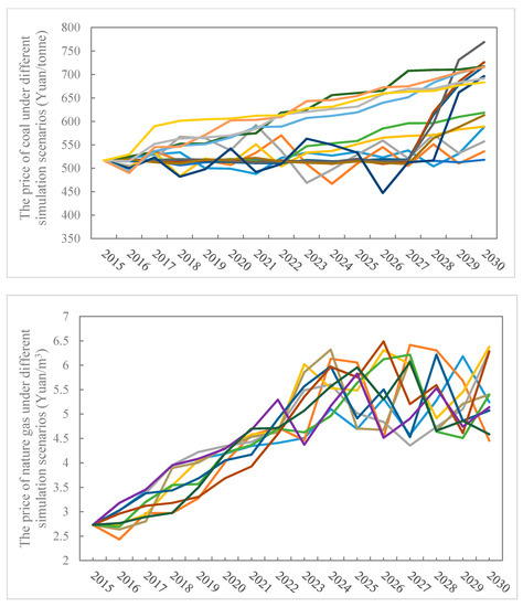
Figure 4.
The prediction price of the fuel under 16 scenarios from 2015~2030.
(2) The output prediction of wind and solar power
Figure 5 shows the output prediction results of the wind and solar power in four seasons under three planning periods. It indicates that both the output of wind and solar power showed seasonal variation. For wind power, the simulation result showed that spring and winter were the main seasons that generate power in Inner Mongolia. Meanwhile, the peak output of wind power varied at different times of the day. For example, in spring, the peak output of the wind power appeared from 5:00 to 9:00 am, while in winter, it appeared from 20:00 to 23:00. Through the adjustment of shape factor and scale factor in period t=2 and t=3, the output simulation in these two periods could be executed. It indicates that the output of the wind power in t=2 and t=3 showed similar performances. The peak output of solar power also varied at different times of the day and different seasons.
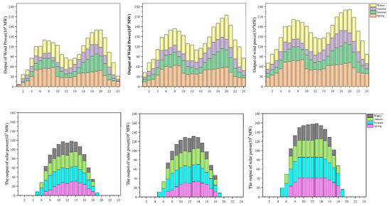
Figure 5.
The output of wind and solar power in different periods (MW).
4.2. The Optimized Electricity Supply and Cooling Technologies
Optimized solutions for electricity supply scheme and cooling technologies in Inner Mongolia are presented in Figure 6. It indicates that the amount of coal-fired power showed a downward trend from t=1 to t=3, while the strict water withdrawals scenario further decreased the amount of coal-fired power generation compared with the flexible one. The average decreasing amplitude under each demand level would be 9%, 5%, and 4% in period t=1, t=2 and t=3, respectively. Gas-fired power, wind power, and solar power showed an increasing trend as time goes on to make up the power generation shortage because of the reduction in coal-fired power. Meanwhile, the electric power production from wind and solar power was larger in the strict water policy scenario than in the flexible one. The phenomena could be attributed to the fact that wind power and solar power consumed no water during the power generation process, so strict water withdrawals policy resulted in more wind and solar power instead of coal-fired and gas-fired power in Inner Mongolia. The distribution of three cooling technologies of coal-fired and gas-fired power in different time periods under different water withdrawals policy and power demand levels is also presented in Figure 5. It indicates that the air-cooling system would play the most important role when the strict water withdrawals policy is executed in Inner Mongolia, especially when the power demand level was medium and high, it increased by 77.53% (medium power demand) and 82.17% (high power demand) when t=1, 69.50% and 71.56% when t=2 and 64.74% and 57.53% when t=3 for the coal-fired power. The phenomenon showed that the strict water policy would be a powerful push on the application of the air-cooling system for coal-fired power. The installation capacity of coal-fired power also showed that as time goes on, the air-cooling system will replace the dominant position of the cycling cooling system and one through system. In 2035, the installation capacity of coal-fired with air-cooling technology would reach 70.64 GWh (flexible scenario) and 116.37 GWh (strict scenario). Meanwhile, the one-through system would gradually be replaced by the other two cooling technologies.
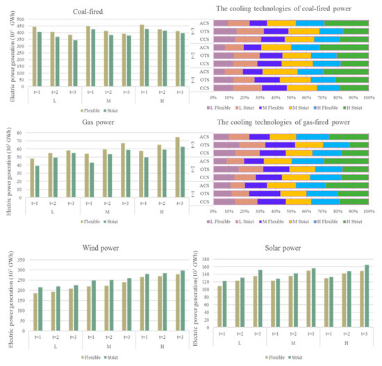
Figure 6.
The optimized electric power generation and capture and storage technology (CCS) scheme (ACS, OTS, and CCS denote the air-cooling system, the one-through system, and the cycling cooling system, respectively).
4.3. Capacity Expansion
The CO2 emissions up to the peak (CEUP) target and water withdrawal policies in the planning periods may greatly impact the power sources structure in Inner Mongolia. We analyzed the distributions of the generation capacity of Inner Mongolia for each technology under four scenarios in 2030 and tried to find out the interactions between the capacity expansion schemes and environmental limits. In Figure 7, the 65% CO2 emissions reduction on the base of 2005 was the CO2 limit. The flexible and strict water withdrawal policies coupled with this CO2 reduction level was chosen to investigate the mixed impact of CO2 and water constraints on the capacity expansion in 2030. The box-and-whisker diagram shows different impacts from different scenarios on the capacity expansion in Inner Mongolia. The boundary closest to zero is the first quartile, the one closest to the top indicates the 75th percentile, and the line within the box marks the median, error bars above and below the box indicate the 90th and 10th percentiles, respectively. Moreover, the dots above or below the error bars represent the 5th and 95th percentiles.
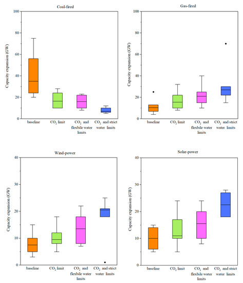
Figure 7.
The capacity expansion under mixed scenarios.
Results indicated that the capacity expansion of different technologies had different appearances in mixed scenarios. Take the coal-fired power as an example, the mid hinge turned into a lower level, which meant the average amount of capacity expansion decreased (nearly 20%~50% reduction), and the dispersion of the distribution mainly aggregated on the low-capacity level (less than 30 GW for the coal-fired power) when the CO2 limit and water constraints were taken into account. The performance of the average amount of the capacity expansion for the CO2 limit and that coupled with the flexible water was approximately the same, although their distribution was different. When the strict water limit was involved, the average amount of capacity expansion showed the lowest level, which was just less than 10 GW. It indicated that the strict water policy dramatically reduced the capacity expansion amount of coal-fired power. For the gas-fired power, the skewness of gas-fired turned to a higher level (increased by 40%) when the CO2 limit was taken into account. Moreover, the capacity expansion would be further promoted when the water limits were present, especially for the strict one.
The other two technologies show the same performance as the gas-fired power, which was in the presence of CO2 limit, the amount of capacity expansion would be promoted, and water limits would further increase the amount of capacity expansion. The reason can be attributed to the fact that coal-fired power has higher CO2 emissions and water withdrawals for cooling. The joint constraints from the CO2 emissions limit and water withdrawals limit will lead to a substantial reduction in CO2 and water withdrawals. Gas-fired and the other two technologies with fewer water withdrawals and emissions will have a large potential to make up the capacity gap when the amount of coal-fired power decrease.
4.4. The CO2 Emissions and Water Withdrawals
The installation level of CCS devices, the amount of CO2 emissions, and the CO2 reduction levels in Inner Mongolia are shown in Figure 8. It indicates that more CCS devices were acquired under the flexible water withdrawals scenario than the strict one. Compared with the flexible scenario, almost 10.19%, 15.78%, and 27.98% fewer CCS devices were required under the strict water scenario when the power demand level was low, medium, and high, respectively. The result indicates that strict water policy not only helps to decrease the water withdrawals but also indirectly leads to the CO2 emissions’ mitigation because of the reduction in the thermal power (coal-fired and gas-fired) installations. With the help of the CCS devices, the CO2 emissions showed a decreasing trend in Inner Mongolia as time goes on to realize the target of reaching the CO2 emissions peak of China in 2030. For example, the amount of CO2 emissions was 10,015 × 1010 tonne in t=1, 9634 × 1010 tonne in t=2, and 8635 × 1010 tonne in t=3 when the power demand level was low, while when the power demand level was high, the CO2 emission was 14795 × 1010 tonne, 12,689 × 1010 tonne, and 11158 × 1010 tonne in t=1,2, and 3, respectively. Meanwhile, the CO2 reduction through the CCS devices showed an increasing trend as time goes on. Higher power demand led to more CO2 emissions reduction to meet the CO2 emissions criteria.
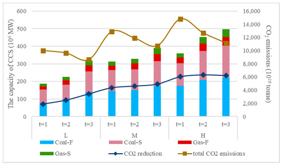
Figure 8.
The installation level of CCS devices and CO2 emissions (-F denotes the flexible water policy scenario, while -S denotes the strict water policy scenario).
The water withdrawals and system cost are shown in Figure 9. It indicates that the strict water policy had an apparent effect on the reduction in water withdrawals than the flexible water policy. For example, the water withdrawals decreased by 41.02%, 48.28%, and 59.07% in t=1,2, and 3 when the power demand was low. The system cost showed an increasing trend as time goes on, and the result also showed that increasing power demand level led to an increase in the system cost. The system cost under the flexible water withdrawal policy led to an average level of 16.32%, 13.76%, and 7.36% reduction than that under the strict policy when the demand level was low, medium, and high. The reason can be attributed to the fact that on the one hand, more air-cooling technologies will take the place of the once-through or the cycling cooling system to reach the water reduction target, which may result in higher system cost; on the other hand, more renewable power technologies, whose water consumption can even be neglected but with higher fixed investment fees, will be applied instead of the thermal power technologies, especially the coal-fired power under the strict water policy, which will further lead to the increase in the system cost. Although the thermal power showed a decreasing trend as time goes on, more CCS devices were still necessary to achieve the more and more strict CO2 emissions target, and this was the third sector, which led to the increase in the system cost. Generally, under the triple constraints of power demand, water policy, and carbon emissions mitigation, more system costs should be invested to help reach the synergetic energy–economy–environment goals in the EPS of Inner Mongolia.
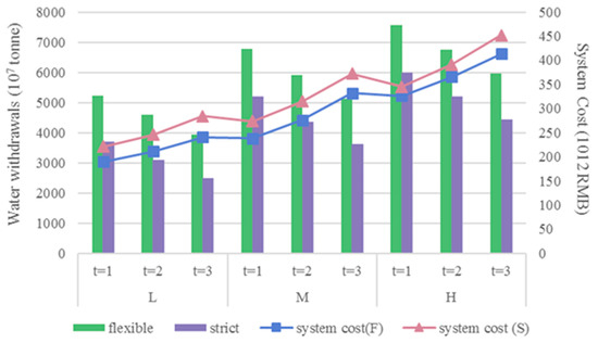
Figure 9.
The water withdrawals and system cost.
4.5. The Optimized Penetration and Satisfaction Degree
The optimized result of renewable energy penetration and satisfaction degree of the system is shown in Table 5. The renewable penetration showed an increasing trend as time goes on, and the strict water withdrawal policy led to a higher renewable penetration rate in each planning period. For example, in t=2, the renewable penetration rate under the strict water policy was 3.58% more than that under the flexible one. However, the satisfaction degree of the system, which implies that each part of the system has reached its best balance, had different performances. The supreme satisfaction degree (λ=0.9523) appeared in t=2 under the strict water withdrawal policy, which means that the renewable penetration rate and the system cost achieved the optimal tradeoff under the CO2 emissions reduction level in the period t=2. The satisfaction degree helps quantize the overall system satisfaction level. Decision-makers can evaluate and adjust their optimized strategies based on the satisfaction degree.
Table 5.
The optimized renewable energy penetration and the satisfaction degree of the system.
5. Conclusions
This study proposed a patron–client interactive optimized (PCIO) model to investigate the energy–water–carbon nexus optimization in Inner Mongolia under the policy background of 2030 CO2 emissions up to the peak target in China, concerning the uncertainty of fuel price and output of the wind and solar power. PICO model not only had the ability to tackle problems with the hierarchical relationship and achieved the proper tradeoffs between maximizing the renewable power penetration and minimizing the system cost but also synergistically dealt with multiple optimized targets, including the power supply and capacity expansion schemes, water consumption control through the combination of different cooling techniques and CO2 emissions mitigation target with the CCS device.
The optimized results indicated that the coal-fired power showed a downward trend during the whole planning horizon under the CEUP target in Inner Mongolia. Gas-fired and renewable power will continuously substitute the place of coal-fired power in this region. The strict water withdrawal policy further exacerbated the substitution effect of the coal-fired power by wind and solar power, with an average level of 9%, 5%, and 4% in three periods. To achieve both the CEUP and water-saving target, the CCS device and the air-cooling system will play gradually important roles in Inner Mongolia’s EPS, especially in the strict water withdrawal scenario, even when the coal-fired power decreases as time goes on. However, these targets will be achieved at the expense of high system costs, which may increase the financial burden of the local government of Inner Mongolia. The PICO model makes it possible to make reasonable tradeoffs between maximizing the renewable energy proportion and minimizing the system costs through the quantized satisfaction degree. Decision-makers can make flexible strategies through the adjustment of the membership function of the PICO model.
As Inner Mongolia is a major energy supply province, which shoulders the responsibility of transferring the electric power resource to other regions (mainly to the Jing-Jin-Hebei region), the potential impacts on the local energy–water–carbon nexus when transmitting energy to other regions should also be taken into consideration. Meanwhile, wind and solar power generation curtailment may also be core concerns with respect to the CEUP target in Inner Mongolia, which will also be investigated in our future studies.
Author Contributions
Conceptualization, Q.T.; Resources, Q.T.; Funding acquisition, Q.T.; Supervision and Review, Q.T.; Methodology, Y.L.; Software, Y.L.; Formal analysis, Y.L.; Writing—original Draft, Y.L.; Writing & Editing, Y.L.; Investigation, J.H. and M.G.; Data Curation, J.H. and M.G. All authors have read and agreed to the published version of the manuscript.
Funding
This research was supported by the National Natural Science Foundation of China (71874053), and the Fundamental Research Funds for the Central Universities (2019QN064).
Acknowledgments
The authors thank the editor and the anonymous reviewer for their helpful comments and suggestions.
Conflicts of Interest
The authors declare no conflict of interest.
References
- Wang, Y.; Su, X.; Qi, L.; Shang, P.; Xu, Y. Feasibility of peaking carbon emissions of the power sector in China’s eight regions: Decomposition, decoupling, and prediction analysis. Environ. Sci. Pollut. Res. 2019, 26, 29212–29233. [Google Scholar] [CrossRef]
- Tao, Y.; Wen, Z.; Xu, L.; Zhang, X.; Tan, Q.; Li, H.; Evans, S. Technology options: Can Chinese power industry reach the CO2 emission peak before 2030? Resour. Conserv. Recycl. 2019, 147, 85–94. [Google Scholar] [CrossRef]
- National Bureau of Statistics. 9–15 Installed Capacity of Power Generation. 2018. Available online: http://www.stats.gov.cn/ (accessed on 13 September 2018).
- Zhang, M.; Liu, X.; Wang, W.; Zhou, M. Decomposition analysis of CO2 emissions from electricity generation in China. Energy Policy 2013, 52, 159–165. [Google Scholar] [CrossRef]
- Zhang, H.; Zhang, X.; Yuan, J. Transition of China’s power sector consistent with Paris Agreement into 2050: Pathways and challenges. Renew. Sustain. Energy Rev. 2020, 132, 110102. [Google Scholar] [CrossRef]
- Ju, L.; Tan, Z.; Li, H.; Tan, Q.; Yu, X.; Song, X. Multi-objective operation optimization and evaluation model for CCHP and re-newable energy-based hybrid energy system driven by distributed energy resources in China. Energy 2016, 111, 322–340. [Google Scholar] [CrossRef]
- Muratori, M.; Kheshgi, H.; Mignone, B.; Clarke, L.; McJeon, H.; Edmonds, J. Carbon capture and storage across fuels and sectors in energy system transformation pathways. Int. J. Greenh. Gas. Control. 2017, 57, 34–41. [Google Scholar] [CrossRef]
- Tan, Q.; Liu, Y.; Ye, Q. The impact of clean development mechanism on energy-water-carbon nexus optimization in Hebei, China: A hierarchical model based discussion. J. Environ. Manag. 2020, 264, 110441. [Google Scholar] [CrossRef]
- Gao, Z.; Geng, Y.; Wu, R.; Chen, W.; Wu, F.; Tian, X. Analysis of energy-related CO2 emissions in China’s pharmaceutical industry and its driving forces. J. Clean. Prod. 2019, 223, 94–108. [Google Scholar] [CrossRef]
- Khan, A.; Chenggang, Y.; Hussain, J.; Bano, S.; Nawaz, A. Natural resources, tourism development, and energy-growth-CO2 emission nexus: A simultaneity modeling analysis of BRI countries. Resour. Policy 2020, 68, 101751. [Google Scholar] [CrossRef]
- Liu, G.; Hu, J.; Chen, C.; Xu, L.; Wang, N.; Meng, F.; Giannetti, B.F.; Agostinho, F.; Almeida, C.M.B.; Casazza, M. LEAP-WEAP analysis of urban energy-water dynamic nexus in Beijing (China). Renew. Sustain. Energy Rev. 2021, 136, 110369. [Google Scholar] [CrossRef]
- Zhai, Y.; Zhang, T.; Bai, Y.; Ji, C.; Ma, X.; Shen, X.; Hong, J. Energy and water footprints of cereal production in China. Resour. Conserv. Recycl. 2021, 164, 105150. [Google Scholar] [CrossRef]
- Tabatabaie, S.M.H.; Murthy, G.S. Development of an input-output model for food-energy-water nexus in the pacific northwest, USA. Resour. Conserv. Recycl. 2020. [Google Scholar] [CrossRef]
- Xu, W.; Xie, Y.; Cai, Y.; Ji, L.; Wang, B.; Yang, Z. Environmentally-extended input-output and ecological network analysis for Energy-Water-CO2 metabolic system in China. Sci. Total. Environ. 2021, 758, 143931. [Google Scholar] [CrossRef] [PubMed]
- Tan, Q.; Liu, Y.; Zhang, X. Stochastic optimization framework of the energy-water-emissions nexus for regional power system planning considering multiple uncertainty. J. Clean. Prod. 2021, 281, 124470. [Google Scholar] [CrossRef]
- Wang, C.; Olsson, G.; Liu, Y. Coal-fired power industry water-energy-emission nexus: A multi-objective optimization. J. Clean. Prod. 2018, 203, 367–375. [Google Scholar] [CrossRef]
- Piao, M.; Li, Y.; Huang, G. Development of a stochastic simulation–optimization model for planning electric power systems—A case study of Shanghai, China. Energy Convers. Manag. 2014, 86, 111–124. [Google Scholar] [CrossRef]
- Emami, J.M.; Ghaderi, S.F.; Sangari, M.S. Integrating energy and water optimization in buildings using mul-ti-objective mixed-integer linear programming. Sustain. Cities Soc. 2020, 62, 102409. [Google Scholar] [CrossRef]
- Sinha, S. Fuzzy programming approach to multi-level programming problems. Fuzzy Sets Syst. 2003, 136, 189–202. [Google Scholar] [CrossRef]
- Chen, Y.; He, L.; Guan, Y.; Lu, H.; Li, J. Life cycle assessment of greenhouse gas emissions and water-energy optimization for shale gas supply chain planning based on multi-level approach: Case study in Barnett, Marcellus, Fayetteville, and Haynesville shales. Energy Convers. Manag. 2017, 134, 382–398. [Google Scholar] [CrossRef]
- Emam, O. A fuzzy approach for bi-level integer non-linear programming problem. Appl. Math. Comput. 2006, 172, 62–71. [Google Scholar] [CrossRef]
- He, L.; Chen, Y.; Ren, L.; Li, J.; Liu, L. Synergistic management of flowback and produced waters during the upstream shale gas operations driven by non-cooperative stakeholders. J. Nat. Gas. Sci. Eng. 2018, 52, 591–608. [Google Scholar] [CrossRef]
- Chen, Y.; He, L.; Li, J.; Lu, H. Stochastic dominant-subordinate-interactive scheduling optimization for interconnected microgrids with considering wind-photovoltaic-based distributed generations under uncertainty. Energy 2017, 130, 581–598. [Google Scholar] [CrossRef]
- Brauneis, A.; Mestel, R.; Palan, S. Inducing low-carbon investment in the electric power industry through a price floor for emissions trading. Energy Policy 2013, 53, 190–204. [Google Scholar] [CrossRef]
- Roy, R.; Jadhav, H. Optimal power flow solution of power system incorporating stochastic wind power using Gbest guided artificial bee colony algorithm. Int. J. Electr. Power Energy Syst. 2015, 64, 562–578. [Google Scholar] [CrossRef]
- Panda, A.; Tripathy, M. Security constrained optimal power flow solution of wind-thermal generation system using modified bacteria foraging algorithm. Energy 2015, 93, 816–827. [Google Scholar] [CrossRef]
- Pau, T. Investigation on Frequency Distribution of Global Radiation Using Different Probability Density Functions. International. J. Appl. Sci. Eng. 2010, 8, 99–107. [Google Scholar]
- Biswas, P.P.; Suganthan, P.; Amaratunga, G.A. Optimal power flow solutions incorporating stochastic wind and solar power. Energy Convers. Manag. 2017, 148, 1194–1207. [Google Scholar] [CrossRef]
- Reddy, S.S.; Bijwe, P.R.; Abhyankar, A.R. Real-Time Economic Dispatch Considering Renewable Power Generation Variability and Uncertainty Over Scheduling Period. IEEE Syst. J. 2015, 9, 1440–1451. [Google Scholar] [CrossRef]
- Standardization Administration. Norm of Water Intake. 2004. Available online: http://www.sac.gov.cn/ (accessed on 15 September 2020).
- State Administration for Market Regulation. Water Saving Enterprises. Fossil Fired Plant; State Administration for Market Regulation: Beijing, China, 2011.
- New.BJX.com.cn. Inner Mongolia: The Installed Capacity of Thermal Power Above 600 MW Reached 81.62 GW. 2018. Available online: http://news.bjx.com.cn/html/20180118/874883.shtml (accessed on 21 November 2020).
- Zhang, J. Analysis of Cost and Policies for CCS. Sino-Global Energy 2010, 3, 21–25. [Google Scholar]
Publisher’s Note: MDPI stays neutral with regard to jurisdictional claims in published maps and institutional affiliations. |
© 2021 by the authors. Licensee MDPI, Basel, Switzerland. This article is an open access article distributed under the terms and conditions of the Creative Commons Attribution (CC BY) license (http://creativecommons.org/licenses/by/4.0/).