Investigation into Sizing Photovoltaic with Energy Storage for Off-Grid Transactive Scenarios ^†

Abstract

In this study, a novel sizing methodology was developed for centralized and interconnected operating strategies of transactive microgrids and several variables were investigated including starting month, initial charge of battery, load variability, unit cost of solar panels and energy storage, number of systems, climate, and required reliability to determine their effect on total cost. The centralized strategy improved cost by seven to ten percent compared to the isolated strategy in every case. The interconnected strategy saved an incremental amount of money consistently compared to the isolated standard. The number of connected systems was not a strong effect. It was thought that increasing the number of systems would increase the benefit of energy sharing. Climate zones studied (“Cold”; “Hot-Dry/Mixed Dry”; “Mixed Humid”; and “Cold but with lower solar irradiation”) showed a large variation on cost with the Hot-Dry/Mixed Dry being the least expensive and Cold, with lower solar irradiation being the most expensive. Cost sensitivity analysis was performed showing that the unit cost of solar has a greater effect on the total cost. Required reliability of power, measured in outage hours, exhibited an inverse relation with cost.

1. Introduction

Historically, residential systems install photovoltaic (PV) energy as a Grid-Connected Photovoltaic (GCPV) system or a Stand-Alone Photovoltaic (SAPV) system. SAPV systems employ solar panels with energy storage systems (ESS) to fulfill load requirements without a connection to a conventional grid system [1]. GCPV systems are connected to external electricity transmission and distribution systems and have no use for their own energy storage. GCPV systems have a distinct advantage because they have backup power readily available and do not need to consider reliability in their design [2].

Consumers and small businesses can save money with the SAPV, provided the cost of generating and storing electricity by your own means is lesser than utility bills through the grid. Making and storing your own electricity is usually more expensive than buying because there is no back up energy available and so any excess generation is wasted, and maintenance and troubleshooting will be significant, enduring problems. Although a recent study of solar plus storage in off-grid residential applications suggested it is not presently cost-effective [3], the cost of solar generation and battery storage is falling [4], while retail electricity prices are rising [5]. SAPV systems make better sense in rural areas where the cost to extend power lines to connect with the grid is onerous (costing between $15,000 and $50,000 each mile) [6].

A transactive microgrid facilitates energy exchanges between otherwise stand-alone systems to try and alleviate the challenges of being independent from a backup energy source. Blockchain has been proven as a technology for facilitating the energy exchanges [7]. Two possible operating strategies for these microgrids include Centralized Energy Sharing (CES), where PV and ESS are centrally located, and Interconnected Energy Sharing (IES), where PV and ESS assets are distributed through the community.

Figure 1 illustrates the CES strategy where individual systems are connected to a centralized solar generation and energy storage system with blockchain technology guaranteeing that each system receives the energy they purchase and only pays for energy they receive. In the CES scenario all loads are combined and considered as one, energy trades are internal and not recorded by the model, and depletion of the energy stored means every customer is without power. Figure 2 illustrates the IES strategy where each customer has their own PV and energy storage with blockchain technology enables energy trades amongst customers.

This “transactive or connected residential microgrid” idea has been investigated, but none of the sources use stochastic numerical analysis to consider year-round off-grid energy sharing strategies. There are many methods for sizing ESS and PV but using stochastic numerical analysis allows for clarity at each hour of the simulation and allows researchers to investigate the trades which occur. The “interconnected sharing mode” proposed by Habib et al. [8] allows residential customers to trade energy to supply their electrical loads in the case that the micro-grid switches to islanded mode during a power outage. A study of 10 houses showed the interconnected sharing case supplied the most load for five out of the 10 houses, three houses preferred isolated self-consumption, and two houses achieved the same load met under either operating mode. The study’s conclusion is that “the interconnected energy sharing case produces only slightly better individual results than the isolated case. However, most importantly, it also led to a 44% reduction in the total size of ESS required.” This research adopts the interconnected sharing mode but allows islanded systems to share their stored energy year-round without connecting to a central grid.

Kalathil et al. [9] studied the Nash equilibrium for investment decisions of a collection of grid-connected firms sharing their energy storage. Akter et al. [10] formulated a mixed-integer linear programming model for optimizing the energy sharing of residential houses to minimize the operational costs of a grid-connected microgrid as well as optimal charging and discharging of energy storages. Starke et al. [11] presented the design and testing of a grid-connected community energy storage system. Huq et al. [12] proposed an energy management system for controlling a community level grid-connected microgrid powered by PV and discuss some of the operational issues which arise. Alsaidan et al. [13] reviewed existing energy storage sizing methods for microgrid applications and proposed a generic sizing method. None of their reviewed papers use a numerical stochastic method to consider combining existing systems for energy sharing.

The goal of this research is to fill the gap in literature by doing initial investigations into energy sharing in year-round off grid transactive microgrids combining existing systems. Many sizing methods for off-grid sizing of ESS and PV have been proposed but none that the authors have found investigate combining existing systems for trading purposes. Specific objectives include (1) develop sizing methodologies for isolated consumption, IES, and CES scenarios; (2) simulate the methodologies considering a range of variables (initial energy storage charge, load variation, unit cost, starting month, number of systems, climate, and required reliability); and (3) compare the cases to determine if energy sharing effectively improves the economics compared to SAPV. This research will enable off-grid community planning, support energy sharing strategy research, and could be incorporated into existing SAPV sizing software.

2. Methodology

2.1. Research Design

The research targets the following research questions: “What type of energy sharing strategy (isolated, IES, or CES) has the lowest total cost? How does the energy sharing strategy, starting month, initial charge, load variation, unit cost, number of systems, geographic location, and required reliability affect total cost and energy storage required?”

The research hypotheses are that the IES and CES operating strategy will reduce the total cost compared to isolated. Increasing the number of systems in IES and CES will reduce the total cost because this will increase the benefit of trading. Additionally, “Hot-Dry/Mixed Dry” climate will have the lowest cost and cost will decrease predictably with lower required reliability. All variables should have some effect on total cost, as given by Equation (1).

Cost = f(Strategy, Month_initial, ESS_initial, Load_var, Cost_unit, N_systems, Location, LPSP_req)

(1)

where Strategy denotes the operating strategy, Month_initial is the starting month, ESS_initial is the initial charge, Load_var designates the type of load variation, Cost_unit designates the unit cost parameters for energy storage and solar, N_systems denotes the number of systems, Location designates the geographic location, and LPSP_req designates the required reliability. One hundred trials were chosen for all cases to ensure convergence of results without significant computation time. A time horizon of one year was chosen for this initial research because this time frame worked best with the existing methodology.

2.1.1. Energy Sharing Strategy

The effect of energy sharing strategy is the focus of this research. For each case below, isolated, IES, and CES operating strategies are considered. The number of systems can only be considered for the IES and CES operating strategies.

2.1.2. Starting Month

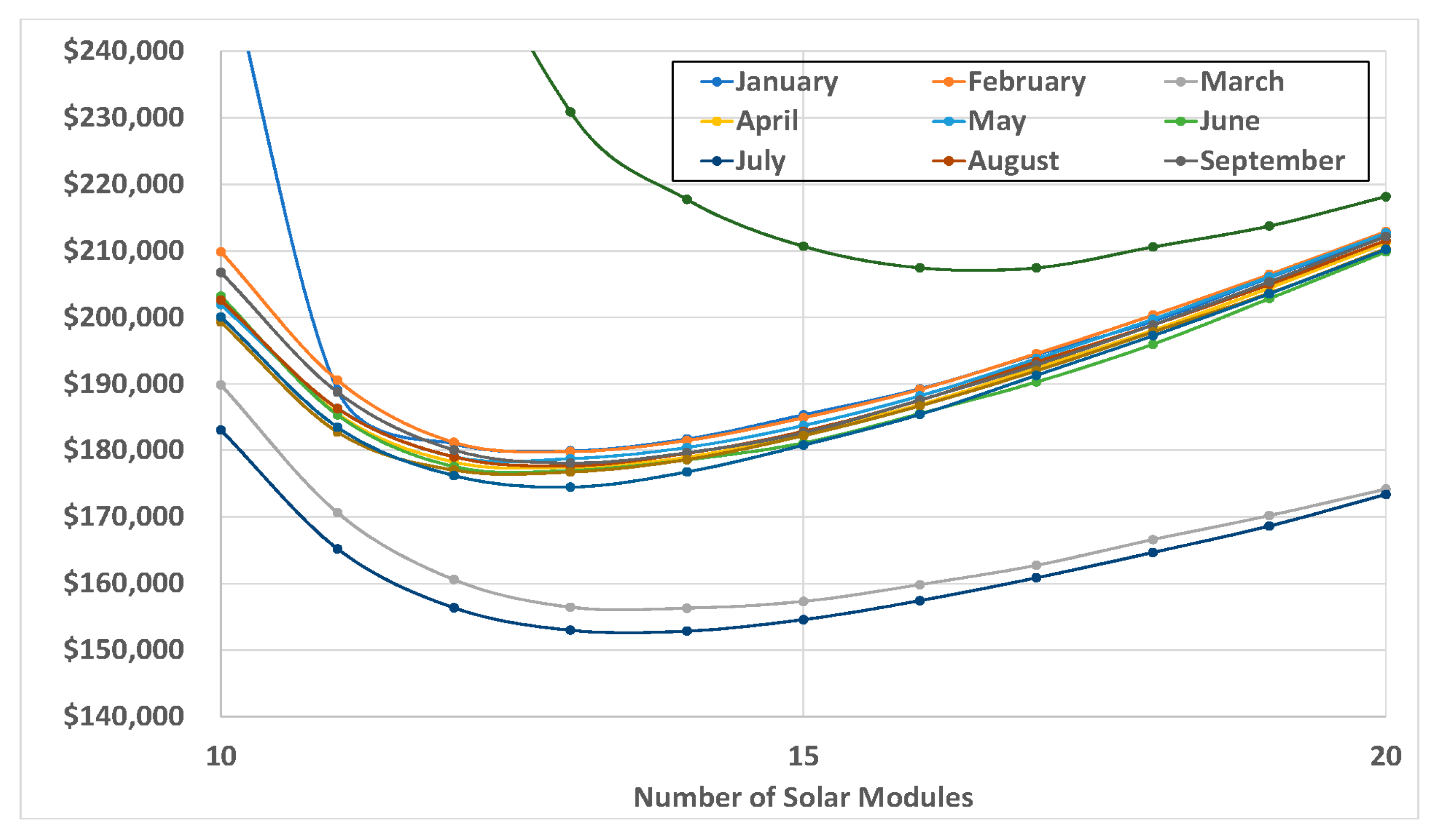
Starting month was chosen as a variable to determine a baseline. The literature was not clear on a typical starting month to choose and if the variable mattered in short-term or long-term simulations. To determine the effect of the starting month (first day of simulation), given as Month_initial, 100 trials were performed for each month (12 cases), with initial charge (10%), number of systems (five), geographic location (Indianapolis), and required reliability (nine hours a year or 0.1% Loss of Power Supply Probability (LPSP)) kept constant. In long term simulations, starting month should not matter after the battery is charged in the initial year. However, initial results show that starting month does have an effect in the short term, especially with low initial charge in a winter month.

2.1.3. Initial Charge

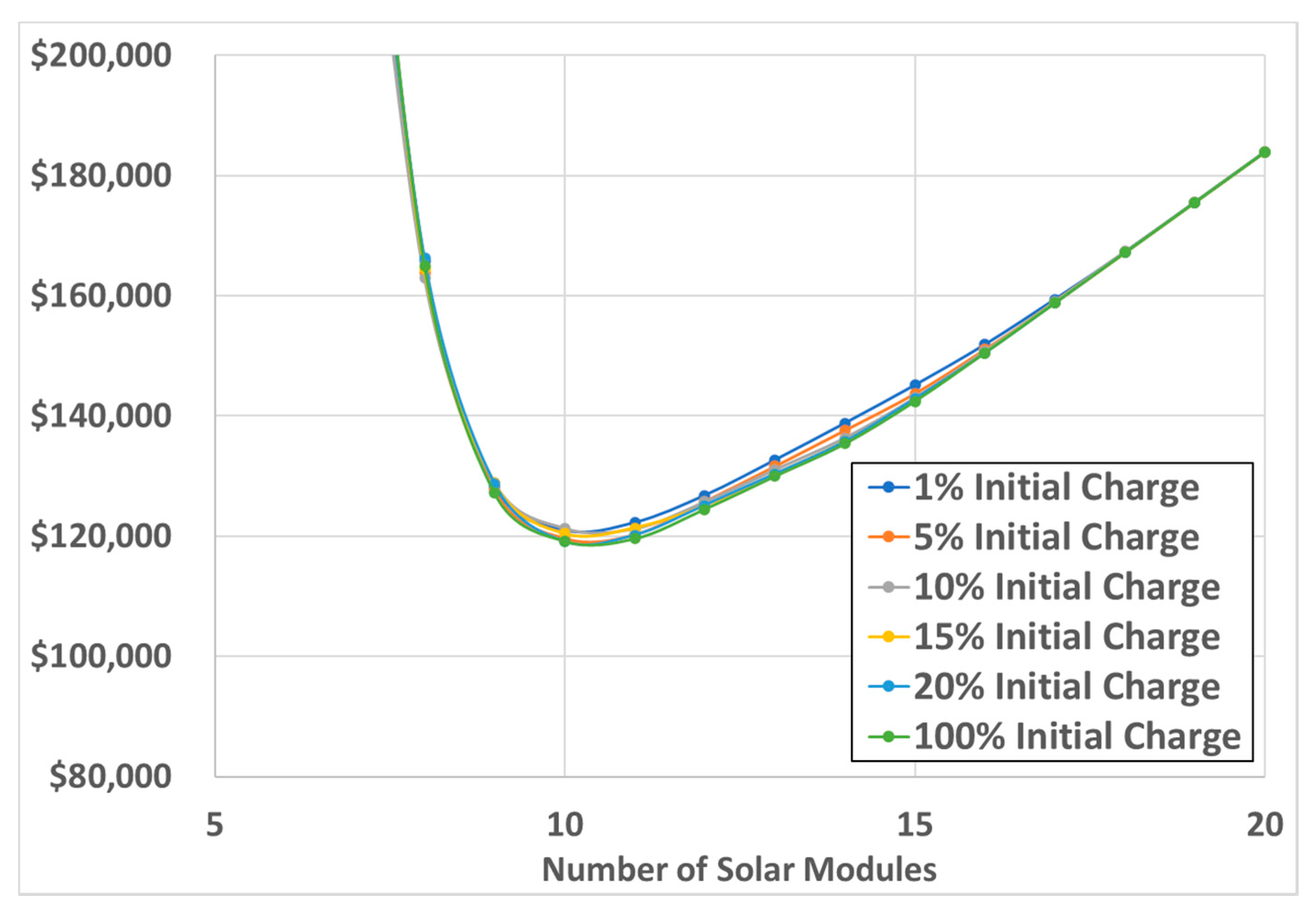
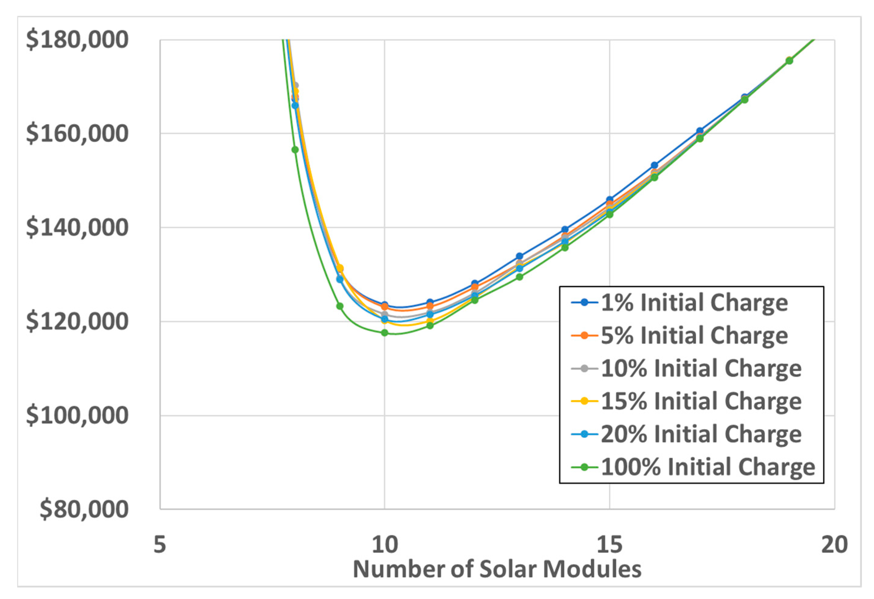
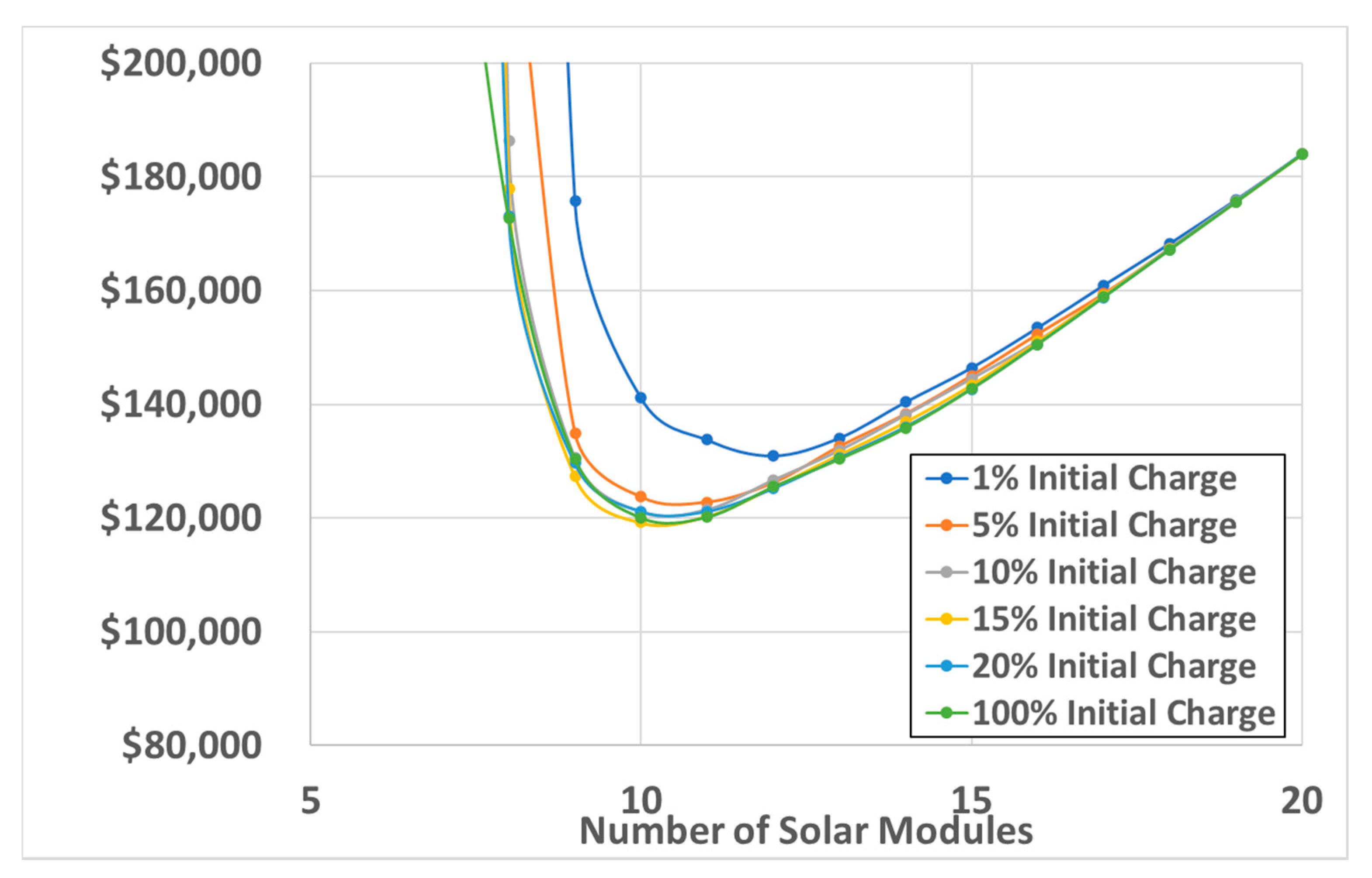
Initial charge, given as ESS_initial, was also chosen to determine a baseline. The literature was not clear on a typical initial charge of a shipped battery. To determine the effect of the initial charge, 100 trials were conducted for each of six cases (1%, 5%, 10%, 15%, 20%, and 100% initial charges) in March, in July, and in November, with number of systems (five), geographic location (Indianapolis), and required reliability (0.1% LPSP) kept constant. Initial charge values were chosen for the typical range (5% to 20%) with an outlier on each end (1% and 100%).

2.1.4. Load Variation

Load variation, given by Load_var, was investigated as the motivational basis for energy trading. If every system has an identical load profile, the simulation would not show any instances where it is beneficial to trade. That situation would not be indicative of real-life load profiles, where different homes have different time schedules. To determine the effect of load variation, 100 trials were conducted for a case with all systems having the same load and a case with all systems having loads simulated by the load simulator, with initial charge (10%), number of systems (five), geographic location (Indianapolis), required reliability (nine hours a year or 0.1% LPSP), and starting month (June) kept constant. The load simulator introduces variability into systems by adding or subtracting a random number of hours, creating the impression that systems are on different schedules.

2.1.5. Cost

The unit cost of the solar panels and energy storage, given by Cost_unit, will change over time for example due to the ending or starting of subsidies, technology improvements, and changes in the market. To show how these changes in cost might affect the analysis, case studies of +/− 15% were included for the energy storage and solar panel unit costs with initial charge (10%), number of systems (five), geographic location (Indianapolis), required reliability (nine hours a year or 0.1% LPSP), and starting month (June) kept constant.

2.1.6. Climate

Climate is known to influence average solar irradiation and hourly load. For example, cold climates typically have lower solar irradiation and higher heating requirements while warmer climates have higher average solar irradiation and higher cooling requirements. To determine the effect of the climate, 100 trials were performed for 4 cases (“Cold”; “Hot-Dry/Mixed”; “Mixed Humid”; and “Cold but with lower solar irradiation”). These cases correspond with Erie, Michigan; Phoenix, Arizona; Little Rock, Arkansas; and Indianapolis, Indiana, respectively.

2.1.7. Number of Systems

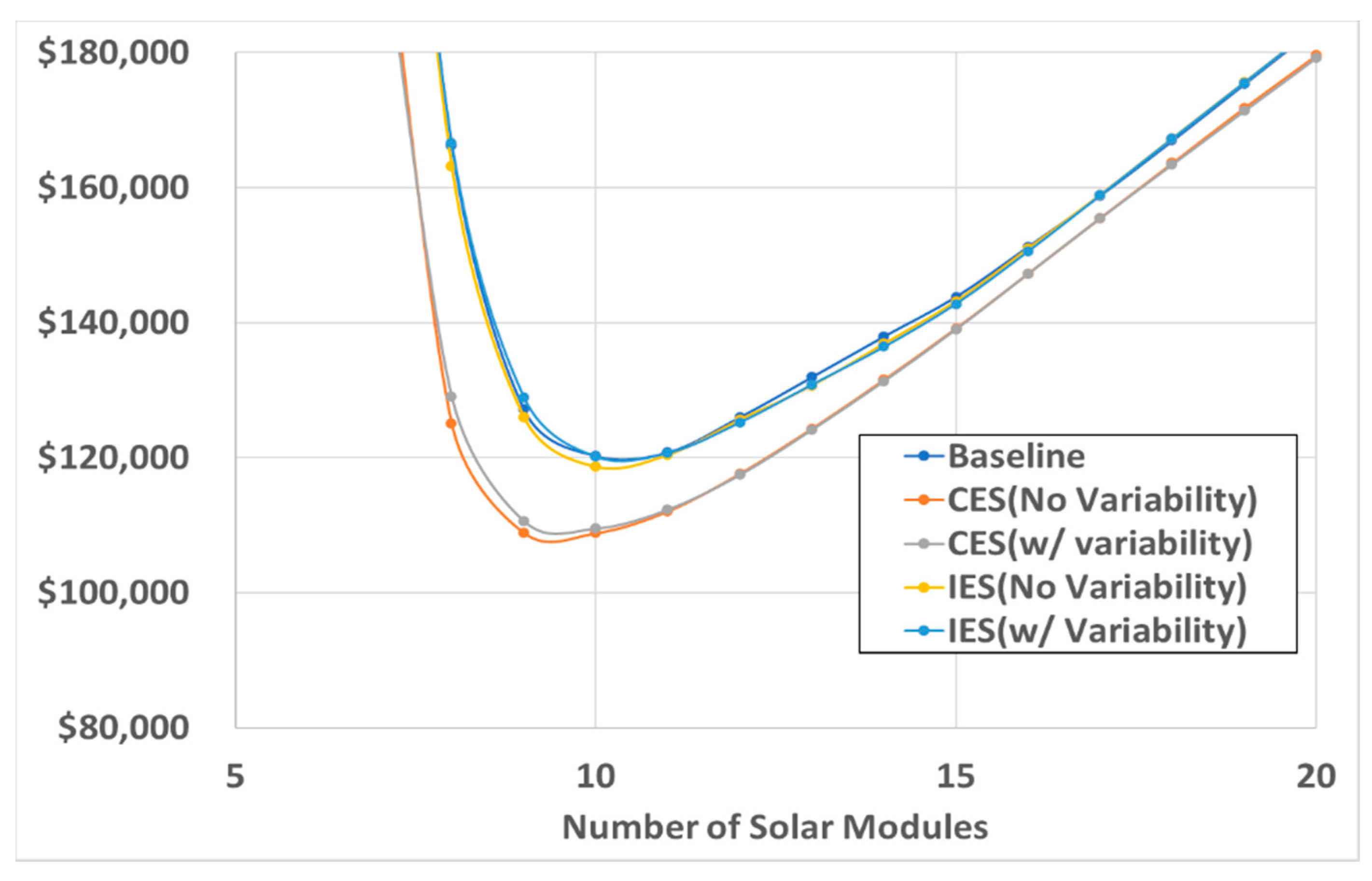
The main simulation studies the size of the community as measured by the number of systems, local climate, and required reliability with starting month (June), and initial charge (10%) kept constant and load variation activated. The number of systems, given by N_systems, was selected because it was believed that more trades would occur and the benefit of establishing a transactive microgrid would improve. To determine the effect of the number of systems, 100 trials were conducted for five cases (N_systems = 2, 5, 10, 20, 50).

2.1.8. Required Reliability

Required reliability, given as LPSP_req, is known to influence amount of energy storage required to ensure that reliability. In 2016 the average US customer experienced 1.3 interruptions for approximately 4 h of outage per year, with significant variability among states and utility providers [14]. A range from nine hours (0.1% LPSP) to ninety hours (1% LPSP) was chosen for this initial investigation.

2.2. Procedure

This section outlines the procedures the model carries out including simulating solar power, simulating hourly load, calculating battery performance, and optimally sizing the energy storage for a given number of solar panels. An overview of the procedure including major input, functions and outputs is given in Figure A1.

2.2.1. Simulating Solar Generation

Solar irradiation data is simulated using Weissbach and King’s Markov model [15] described in Figure A2 and Figure A3. This approach generates reasonable results, though not suitable for sizing specific sites. There is another method given by Chamola and Sikdar [16] that improves Weissbach and King’s Markov model, but it is for dimensioning high-reliability systems.

From the simulated solar irradiation data, power generation is calculated at each hour from Equation (2).

$${\mathrm{P}}_{\mathrm{PV}}={\mathrm{Y}}_{\mathrm{PV}}{\mathrm{f}}_{\mathrm{PV}}\left(\frac{{\mathrm{G}}_{\mathrm{T}}}{{\mathrm{G}}_{\mathrm{T},\mathrm{STC}}}\right)$$

(2)

where P_PV is the output of the PV array in kW. Y_PV is the rated capacity of the PV array under standard conditions. The PV de-rating factor, given by f_PV considers all losses in AC power generation from the solar panel including losses due to temperature [17]. G_T is the simulated solar irradiation in the current time step in W/m². Finally, G_T,STC is the solar irradiation at standard conditions (1000 W/m²). The model does not consider temperature or tilt of the solar panel.

2.2.2. Simulating Residential Load

Simulated residential load is originally taken straight from the input data with variability introduced by adding or subtracting a random number of hours within a range of −3 to +3. This generates the effect of residential households being on different schedules. The load simulation was improved based on initial results to perform a range of variations, horizontal and vertical, based on user input, or randomly within a range. In the CES case, systems are combined into one, having a combined energy generation and load. The IES case uses the same load profiles as the baseline. Figure 3 shows example load variations performed on a 24-h time frame. The blue “Baseline” shows an example 24-h load without any variance. There is typically a small peak when residents are getting ready for work and a larger peak later in the afternoon when they return. The orange line shows a load profile shifted “horizontally” two hours ahead. The peaks occur at hour 6 and 17 instead of 8 and 19. The yellow line shows a load profile shifted “vertically” by 0.3 kWh. The peaks occur at the same time as the baseline but are larger.

2.2.3. Calculating Battery Performance

At each hour, the energy available in the battery is calculated by Equation (3).

$${\mathrm{E}}_{\mathrm{Stored}}={\mathrm{E}}_{\mathrm{Stored}}^{\prime }+\left({\mathrm{P}}_{\mathrm{PV}}-{\mathrm{P}}_{\mathrm{Load}}\right)\times {\mathrm{B}}_{\mathrm{EFF}}$$

(3)

where E_Stored is the output energy available in the current time step. This value is constrained between the battery full capacity and zero charge. E’_Stored is the energy available in the previous time step. P_PV is the output of the PV array in the current time step calculated from Equation (1). P_Load is the simulated load at the current time step. B_EFF is the battery efficiency for charge and discharge. The model does not consider temperature, maximum charge or discharge current, capacity ratio, or the battery’s power to energy ratio.

2.2.4. Optimizing Number of Batteries

The solar power and hourly load are simulated using the methods outlined above. The battery state of charge (SOC) starts at a specified initial charge and is computed at each time step from (2). If battery SOC equals 0% in the current time step a “loss of storage” count is incremented. If the reliability requirement is unsatisfied the battery is incremented, and analysis is repeated. The reliability requirement parameter for this model is Loss of Power Supply Probability (LPSP). LPSP is a widely used method for sizing SAPV systems where 9 h of outage per year means a value of 0001. LPSP, given by Equation (4),

$$\mathrm{LPSP}=\frac{N_{outage}}{N_{total}};0\le \mathrm{LPSP}\le 1$$

(4)

is the ratio of number of hours of outage to the total number of hours considered in the time period [18]. Once the reliability requirement is satisfied, the output is a table giving results for that trial. IES and CES use similar techniques but the hourly load is handled differently, and in IES the systems can trade with each other to prevent having zero SOC. The procedure for baseline, IES, and CES systems are described in more detail in Figure A4 and Figure A5.

In this calculation it is critical to note that we are considering the time sensitivity of the variables and not the amount of energy produced. For example, the LPSP may be nonzero even if energy supply exceeds energy demand, depending on the seasonal nature of the solar energy being generated.

The optimal solution for number of solar panels and amount of energy storage would be the one with a minimum total cost. Cost is given as the initial cost of the system including the cost for all solar panels, all batteries, their installation and hardware, and the interconnection cost.

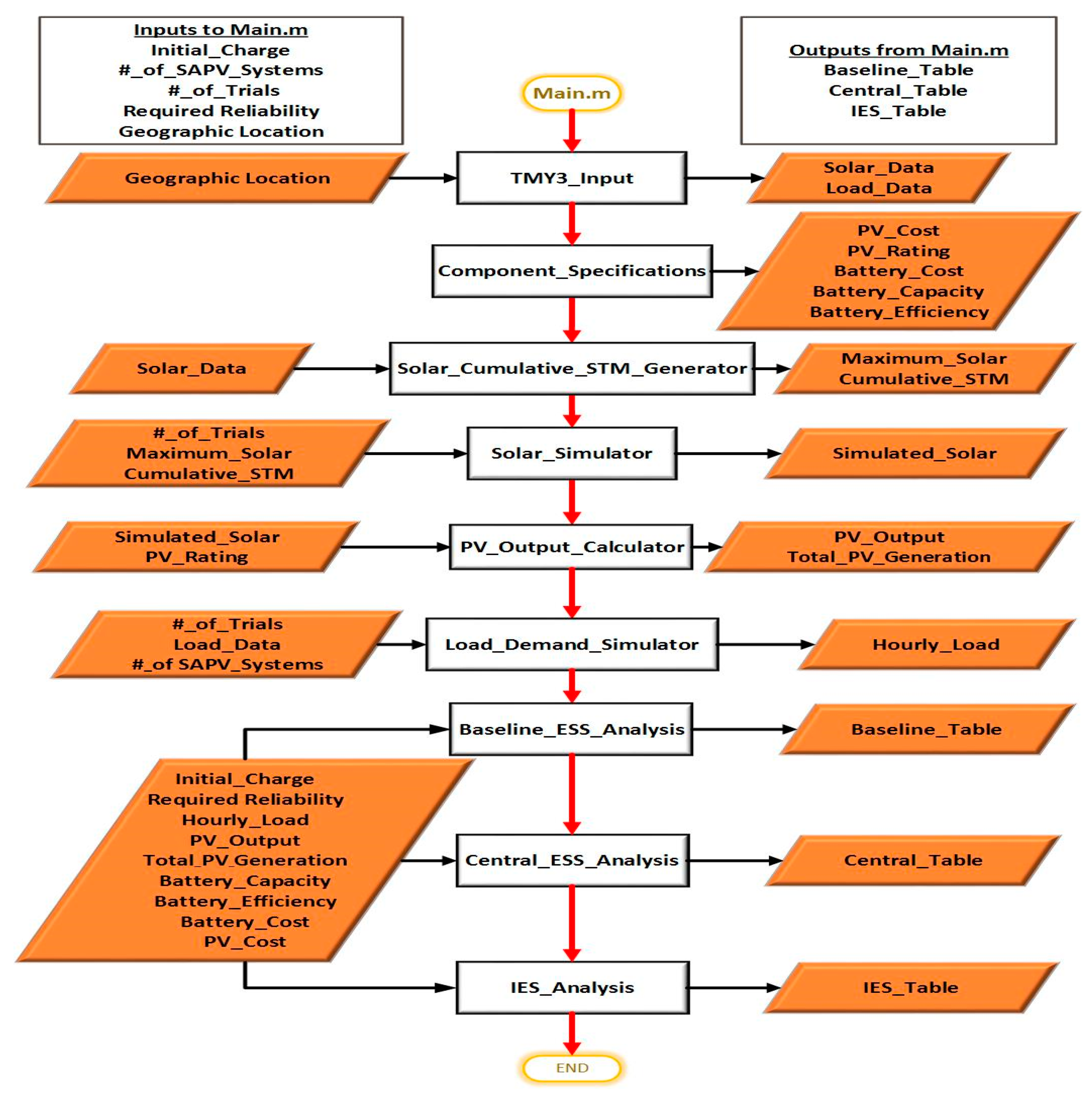
2.3. Inputs

The model inputs are project specifications, component specifications, solar irradiation data, and residential load data. Independent variables include the number of SAPV systems in the community, the number of trials, the acceptable number of outage hours, the number of years being simulated, the insolation data, the load profiles, the initial charge of battery and the starting month of simulation. Component specifications include the solar panel and energy storage performance and cost parameters, given in

Table 1. Photovoltaic (PV) and Energy Storage System (ESS) performance parameters.

Input	Value	Source
Solar Panel Rating	3 kW	[19]
PV De-rating Factor	0.731	[17]
Battery Capacity	13.5 kWh	[20]
Battery Efficiency	90%	[20]

and

Table 2. PV and ESS cost parameters.

Input	Value	Source
Unit Cost (PV)	$4877	[19]
Hardware Cost (PV)	$500	[19]
Installation Cost (PV)	$3000	[19]
Unit Cost (ESS)	$5900	[20]
Hardware Cost ESS	$700	[20]
Installation Cost ESS	$1500	[20]
Interconnection Cost	$200/System	Typical Estimate

, respectively. The solar panel specifications correspond with a 3 kW solar module kit that includes an inverter and racking system [19]. The battery specifications correspond with a 13.5 kWh Tesla Powerwall with an included charge controller assumed to be 100% dischargeable that does not require an enclosure [20]. Battery efficiency is the “round-trip efficiency” considering both charging and discharging. The interconnection cost is a rough estimate taken as $200 assuming that the houses are 50 feet apart, $1/foot of wire, and $150 for installation. The interconnection cost estimate could be improved with a more specific estimate of implementing the Blockchain technology and more knowledge of what controllers are necessary.

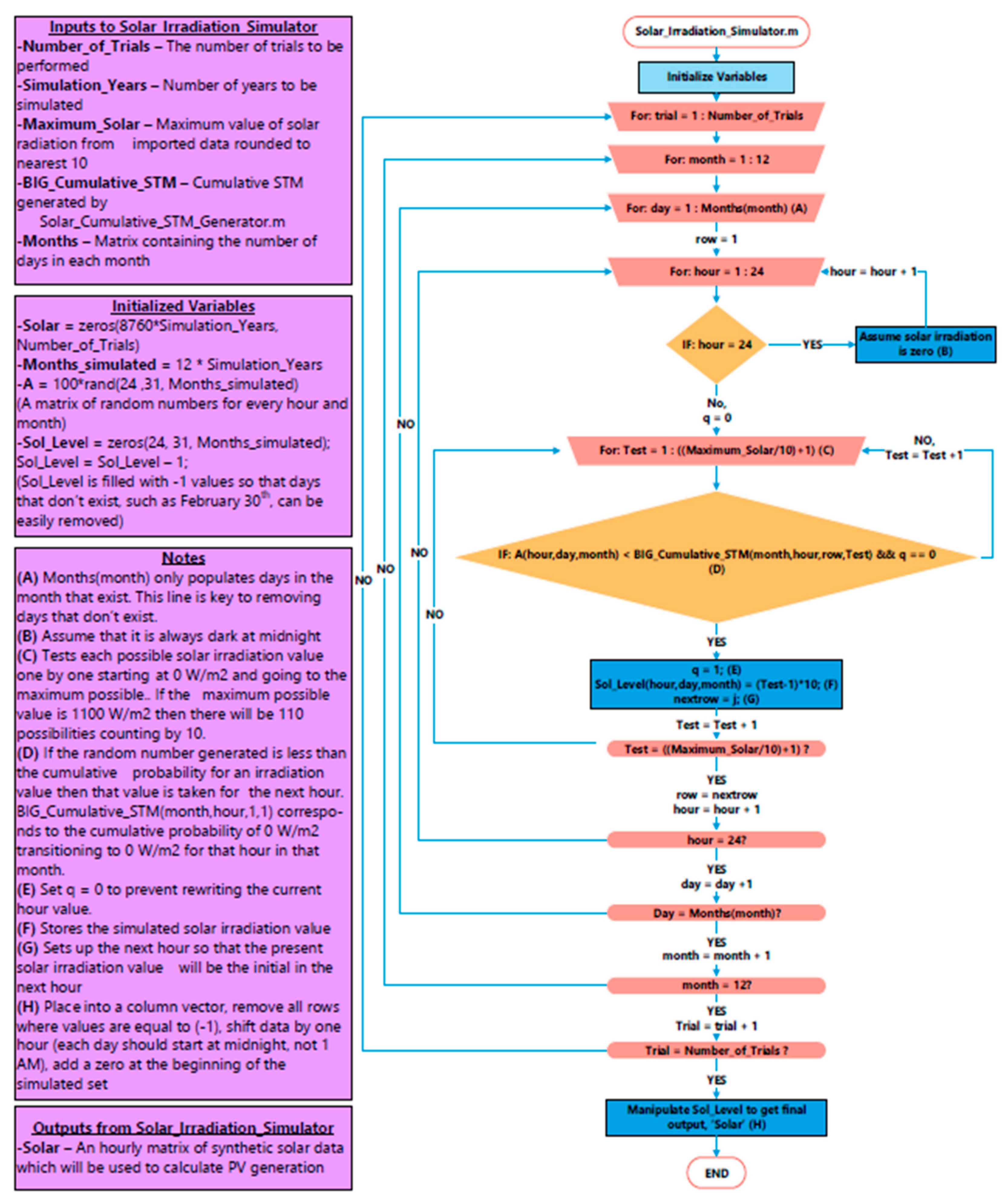
Typical Meteorological Year (TMY) data sets were used for solar irradiation data, specifically TMY3. Although not designed to consider meteorological extremes, TMY data exhibit diurnal and seasonal variations, and they represent a full calendar year of typical climatic conditions for a given location [21]. TMY3 residential load data was selected because it coincides with TMY3 solar data, is freely available, and is in a convenient format. This dataset includes high and low residential hourly load profiles which will be useful for future work [22]. There are five climate zones in the U.S (Marine, Hot-Dry/Mixed-Dry, Hot/Humid, Mixed/Humid, and Cold/Very Cold) from which were selected the sites and simulates residential load data [23]. Each climate zone will have a different typical load profile.

Specific locations are chosen because they all have Class 1 (low uncertainty) data, represent a range of different yearly average Global Horizontal Irradiance (GHI) values, and provide samples from several climate zones. The four locations chosen include Erie, Pennsylvania (Cold); Indianapolis, Indiana (Cold); Little Rock, Arkansas (Mixed-Humid); and Phoenix, Arizona (Hot/Mixed Dry). The purpose of choosing multiple geographic locations was to show that the results are repeated among different data sets and that climate has a noticeable effect. San Antonio, Texas was chosen initially but was abandoned because the load data was discovered to have non-representative values (6.5 kWh days) resulting in much larger capital cost estimates (greater than $200,000). San Antonio was, however, used for validation because it provided a valuable example of how starting month and load variability could affect total cost.

2.4. Validation

Functions were validated by selecting inputs that allowed for confirming the expected output. The methods used for validation are available at [24]. HOMER [25] was chosen as an external validation source because it is accepted as the world’s leading microgrid modeling software company and it performs a related analysis to the proposed model (hourly numerical analysis). No existing commercial software allows for transactive microgrid modeling or simulating the energy trading between systems within a community. Because HOMER cannot simulate an energy trading system or more than one residential system, it can only be used to verify the Baseline (isolated) case. This validation also works to compare our optimal results with an established existing method. HOMER was setup to mimic PV and ESS performance parameters given in Table 1 and Table 2:

• Tesla Powerwall 2.0. Capital cost changed to $8100, search space integers from 1 to 30, and changed the initial state of charge to match the different cases.
• “Large free Converter” component included to model the integrated inverter.
• The same load and solar data used for both models. The load data is larger than HOMER’s initial estimate, but our data includes electric heating.
• “Generic flat plate PV” component used for the PV generation. Changed the PV capacity to 3 kW, capital cost to $8377, derating factor to 73.1%, and edited the search space to only give answers our model would look at. The temperature effects were not considered.
• HOMER does not consider the effect of starting month, so June was taken as the starting month for our baseline model based on preliminary results.
• Case studies considered:

  ○

  Geographic Locations: Phoenix, Arizona; Little Rock, Arkansas; Indianapolis, Indiana; Erie, Pennsylvania

  ○

  Required Reliability: 0.1%, 1% LPSP

  ○

  Initial Charge: 10%, 20%, 100%

These case studies were selected in order to validate whether the developed model compares with HOMER. The geographic locations were selected because they all have Class 1 (lowest uncertainty) data from TMY3, they represent a range of different yearly Global Horizontal Irradiance (GHI) values, and they offer examples from several climate zones. The validation results for Phoenix and Erie are included in

Table 3. Validation of sizing model using HOMER software.

Method	Location	LPSP (%)	Initial Charge (%)	Capital Cost ($)
HOMER	Phoenix, AZ	0.1	10	$74,562
Baseline	Phoenix, AZ	0.1	10	$67,805
HOMER	Phoenix, AZ	0.1	20	$74,562
Baseline	Phoenix, AZ	0.1	20	$67,319
HOMER	Phoenix, AZ	0.1	100	$74,562
Baseline	Phoenix, AZ	0.1	100	$66,995
HOMER	Phoenix, AZ	1	10	$66,185
Baseline	Phoenix, AZ	1	10	$58,051
HOMER	Phoenix, AZ	1	20	$66,185
Baseline	Phoenix, AZ	1	20	$57,970
HOMER	Phoenix, AZ	1	100	$66,176
Baseline	Phoenix, AZ	1	100	$57,808
HOMER	Erie, PA	0.1	10	$133,201
Baseline	Erie, PA	0.1	10	$134,011
HOMER	Erie, PA	0.1	20	$124,824
Baseline	Erie, PA	0.1	20	$133,444
HOMER	Erie, PA	0.1	100	$124,824
Baseline	Erie, PA	0.1	100	$133,768
HOMER	Erie, PA	1	10	$116,724
Baseline	Erie, PA	1	10	$118,992
HOMER	Erie, PA	1	20	$116,724
Baseline	Erie, PA	1	20	$118,020
HOMER	Erie, PA	1	100	$116,724
Baseline	Erie, PA	1	100	$118,263

. Results for Little Rock and Indianapolis can be found at [24]. The average percent difference for each location are approximated as follows: 6% for Erie, 9% for Phoenix, 21% for Indianapolis, and 5% for Little Rock. Some of the differences between the two models are that HOMER calculates reliability through capacity shortage (capacity loss/total capacity demanded) while this study measured hours of service (hours where capacity is lost/8760). It may also be due to the simulation model, battery model, and better optimization model of HOMER. HOMER selects an optimum integer value for the number of batteries while the proposed model takes an average of all the trials, resulting in non-integer values. HOMER does not contain a method for analyzing the starting month of the simulation [25]. These results suggest that starting month should be considered when a system wants to go off-grid particularly in the winter months, because there is less solar power available, which may require additional battery storage during the first winter of operation.

3. Results and Discussion

In this section, results will be produced according to the research design to demonstrate the differences in Baseline (isolated), CES, and IES operating strategies.

3.1. Starting Month

It was found that the months of January, February, March, July, and December give distinct results compared to the other months, which compare very reasonably. Indianapolis (Figure 4) and San Antonio (Figure 5) did not show the same effect for every month. Considering both geographic location results, the month of June was selected as the baseline month for the rest of the simulation.

3.2. Initial Charge

The initial charge effect is not very pronounced in July (Figure 6) or March (Figure 7) but is much more appreciable in November (Figure 8). More research is needed to show how initial charge might affect the remaining months in the year.

In the November case, the lower initial charges of 1% and 5% result in a higher cost, presumably due to the problem of generating enough energy to recover from the initial charge condition.

In the March and July cases, every initial charge condition gives approximately the same cost, showing that there was ample solar energy available to recover from the initial charge condition.

The cases of 1%, 5%, and 100% initial charge show varying results but are not likely scenarios in the real world. The purpose of including these cases was to show that initial charge could have a noticeable effect on initial cost. Ten percent was chosen as the initial charge for the remainder of the simulation.

3.3. Load Variation

Load offset refers to homeowners having similar load profiles that are offset in time due to varying schedules such as arriving home at different times of the day. Ideally, load offset would greatly reduce the capital cost because systems that are not on an identical schedule have more chances to save money by trading. The no-offset case is not a realistic situation; there will almost surely be some load variation between systems.

Varying load offset for San Antonio (Figure 9) indicates that the capital cost is reduced in both the CES with offset and IES with offset cases. For IES with no load offset, it is immediately obvious that there is no reason to establish a transactive microgrid because it costs more than the baseline case. These results are not consistent when geographic location is changed to Indianapolis (Figure 10) which suggests that more simulations are required to verify the effect of load offset.

3.4. Load Variation (Improved)

Because the results of the initial load offset simulation were not consistent between the two geographic locations, more research was necessary to determine the effect of load variability. A new load simulation technique was added that allowed the user to input an amount of variation and a timestep, for example, a random vertical variation of (+/−) 0.3 kWh every 24 h. Results from these case studies are included in

Table 4. Summary of load variability case studies in Indianapolis given 5 systems, starting month of June, 0.1% LPSP required, 100 trials, and 10% initial battery charge.

Case Study	Lowest Average Cost Found
Baseline	$120,301
CES (No Variability)	$110,052
IES (No Variability)	$121,199
CES (Random Horizontal Variation)	$109,080
IES (Random Horizontal Variation)	$119,156
CES (Daily Vertical +/− 0.3 kWh)	$109,226
CES (Hourly Vertical +/− 0.3 kWh)	$110,862
CES (Yearly Vertical +/− 0.3 kWh)	$110,781
IES (Daily Vertical +/− 0.3 kWh)	$118,832
IES (Hourly Vertical +/− 0.3 kWh)	$121,813
IES (Yearly Vertical +/− 0.3 kWh)	$119,529
CES (Daily Vertical +/− 0.6 kWh)	$111,397
CES (Hourly Vertical +/− 0.6 kWh)	$110,279
CES (Yearly Vertical +/− 0.6 kWh)	$114,896
IES (Daily Vertical +/− 0.6 kWh)	$120,145
IES (Hourly Vertical +/− 0.6 kWh)	$120,533
IES (Yearly Vertical +/− 0.6 kWh)	$121,019
CES (Daily Vertical +/− 0.9 kWh)	$113,179
CES (Hourly Vertical +/− 0.9 kWh)	$110,230
CES (Yearly Vertical +/− 0.9 kWh)	$119,448
IES (Daily Vertical +/− 0.9 kWh)	$122,463
IES (Hourly Vertical +/− 0.9 kWh)	$120,728
IES (Yearly Vertical +/− 0.9 kWh)	$121,993

.

The cost did not go down with increasing amounts of vertical variation as expected. Instead, the CES with random horizontal variation showed the lowest average cost and was not as low as the initial results showed. This indicates that the vertical load variability did not have the effect that was hypothesized. Neither the IES nor CES case with variability was able to improve upon the case without variability. This result indicates that there is not an added benefit of establishing a transactive microgrid between SAPV systems which have varying load profiles. However, there is still a consistent and predictable savings associated with the CES case over the IES and baseline.

3.5. Cost

The impact of change in energy storage and solar panel unit cost is shown in

Table 5. Results of varying unit cost of energy storage and solar panels in Indianapolis given 5 systems, starting month of June, 0.1% LPSP required, 100 trials, and 10% initial battery charge.

Method	Solar Cost	Battery Cost	Number of Solar Panels	Number of Batteries	Capital Cost ($/System)
CES	−15%	−15%	10	3.1	$99,050
CES	−15%	+0%	10	3.1	$101,457
CES	−15%	+15%	10	3.0	$103,969
CES	+0%	−15%	10	3.1	$106,149
CES	+0%	+0%	10	3.2	$109,679
CES	+0%	+15%	10	3.0	$111,105
CES	+15%	−15%	10	3.2	$114,258
CES	+15%	+0%	10	3.1	$116,768
CES	+15%	+15%	10	3.1	$119,768
IES	−15%	−15%	10	4.5	$108,819
IES	−15%	+0%	10	4.3	$111,517
IES	−15%	+15%	10	4.4	$112,277
IES	+0%	−15%	10	4.4	$115,471
IES	+0%	+0%	10	4.5	$120,307
IES	+0%	+15%	10	4.3	$122,552
IES	+15%	−15%	10	4.5	$123,970
IES	+15%	+0%	10	4.5	$127,995
IES	+15%	+15%	10	4.4	$130,981

. The results show predictably higher cost with higher unit cost of solar and battery. The price of solar has a larger effect on these results, for instance, by comparing the case where solar is 15% less and battery is the same with the case where solar is the same and battery is 15% less. Although the unit price of solar panels is smaller than that of batteries, there are more of them in the optimal solution. It was expected that the number of batteries would decrease as the cost went up, but this result was inconsistent due to the optimization and small change in cost. A larger change in unit cost should be considered.

3.6. Climate

The effect of climate is explored by choosing four U.S. locations with a variety of climate zones and average solar irradiation levels. The results for the locations chosen (Indianapolis, Erie, Phoenix, and Little Rock) are shown in

Table A1. Summary table for Indianapolis showing average lowest cost configuration for each case.

Operating Strategy	LPSP (%)	# of Systems	# of Solar Panels	# of Batterie (Average)	Capital Cost (Average)
Isolated	0.1	-	10	4.5	$120,301
Isolated	0.2	-	10	4.2	$117,709
Isolated	0.5	-	10	3.3	$110,662
Isolated	1	-	9	3.5	$103,338
IES	0.1	2	10	4.4	$119,691
IES	0.1	5	10	4.5	$120,161
IES	0.1	10	10	4.3	$119,035
IES	0.1	20	10	4.1	$117,188
IES	0.1	50	10	4.2	$117,630
IES	0.2	2	10	4	$116,532
IES	0.2	5	10	4	$116,435
IES	0.2	10	10	4.1	$117,059
IES	0.2	20	10	3.9	$115,884
IES	0.2	50	10	4	$116,540
IES	0.5	2	10	3.2	$109,931
IES	0.5	5	10	3.3	$111,056
IES	0.5	10	10	3.2	$109,769
IES	0.5	20	10	3.1	$109,426
IES	0.5	50	10	3.1	$109,048
IES	1	2	9	3.6	$104,713
IES	1	5	9	3.6	$104,397
IES	1	10	9	3.2	$101,116
IES	1	20	9	3.3	$102,319
IES	1	50	9	3.2	$101,703
CES	0.1	2	10	3.3	$110,903
CES	0.1	5	10	3.2	$109,517
CES	0.1	10	10	3.1	$108,716
CES	0.1	20	9	3.9	$107,337
CES	0.1	50	10	2.9	$108,168
CES	0.2	2	9	4	$107,912
CES	0.2	5	9	3.8	$106,567
CES	0.2	10	9	3.8	$106,584
CES	0.2	20	10	2.7	$106,067
CES	0.2	50	10	2.8	$106,519
CES	0.5	2	9	3	$99,974
CES	0.5	5	9	3.1	$100,314
CES	0.5	10	9	2.8	$98,411
CES	0.5	20	9	2.8	$97,917
CES	0.5	50	9	2.8	$98,352
CES	1	2	9	2.4	$95,317
CES	1	5	9	2.3	$94,110
CES	1	10	9	2.1	$92,611
CES	1	20	9	2.1	$92,814
CES	1	50	9	2.1	$92,739

,

Table A2. Summary table for Erie showing average lowest cost configuration for each case.

Operating Strategy	LPSP (%)	# of systems	# of Solar Panels	# of Batteries (Average)	Capital Cost (Average)
Isolated	0.1	-	13	3	$133,282
Isolated	0.2	-	13	2.7	$131,014
Isolated	0.5	-	12	3	$125,148
Isolated	1	-	12	2.3	$118,911
IES	0.1	2	13	3	$133,037
IES	0.1	5	13	3	$132,980
IES	0.1	10	13	2.9	$132,696
IES	0.1	20	13	2.9	$132,283
IES	0.1	50	13	2.8	$131,800
IES	0.2	2	13	2.5	$129,149
IES	0.2	5	13	2.5	$129,675
IES	0.2	10	13	2.5	$129,132
IES	0.2	20	13	2.4	$128,496
IES	0.2	50	13	2.5	$128,965
IES	0.5	2	12	2.8	$123,688
IES	0.5	5	12	2.8	$123,534
IES	0.5	10	12	2.8	$123,582
IES	0.5	20	12	2.8	$123,594
IES	0.5	50	12	2.7	$122,719
IES	1	2	12	2.1	$117,815
IES	1	5	12	2.1	$117,766
IES	1	10	12	2	$117,621
IES	1	20	12	2.1	$117,702
IES	1	50	12	2	$117,204
CES	0.1	2	12	2.8	$123,526
CES	0.1	5	12	2.6	$121,719
CES	0.1	10	12	2.6	$121,800
CES	0.1	20	12	2.5	$121,010
CES	0.1	50	12	2.4	$120,540
CES	0.2	2	12	2.4	$120,083
CES	0.2	5	12	2.2	$118,933
CES	0.2	10	12	2.2	$118,641
CES	0.2	20	12	2.1	$118,026
CES	0.2	50	12	2.2	$118,312
CES	0.5	2	12	2.2	$117,167
CES	0.5	5	12	1.8	$115,320
CES	0.5	10	12	1.8	$114,972
CES	0.5	20	12	1.8	$115,025
CES	0.5	50	12	1.7	$114,688
CES	1	2	11	2.2	$110,289
CES	1	5	11	2	$108,822
CES	1	10	11	2	$108,345
CES	1	20	11	2	$108,644
CES	1	50	11	1.9	$108,048

,

Table A3. Summary table for Phoenix showing average lowest cost configuration for each case.

Operating Strategy	LPSP (%)	# of Systems	# of Solar Panels	# of Batteries (Average)	Capital Cost (Average)
Isolated	0.1	-	4	4	$65,908
Isolated	0.2	-	4	3.8	$64,126
Isolated	0.5	-	4	3.2	$59,752
Isolated	1	-	4	3	$57,970
IES	0.1	2	4	4.1	$66,756
IES	0.1	5	4	3.8	$64,358
IES	0.1	10	4	4	$66,278
IES	0.1	20	4	3.8	$64,666
IES	0.1	50	4	3.8	$64,865
IES	0.2	2	4	3.7	$63,759
IES	0.2	5	4	3.5	$61,815
IES	0.2	10	4	3.5	$62,074
IES	0.2	20	4	3.4	$61,199
IES	0.2	50	4	3.4	$61,191
IES	0.5	2	4	3.1	$59,142
IES	0.5	5	4	3.1	$59,093
IES	0.5	10	4	3.2	$59,385
IES	0.5	20	4	3.1	$58,522
IES	0.5	50	4	3.1	$58,638
IES	1	2	4	2.9	$57,198
IES	1	5	4	2.8	$56,485
IES	1	10	4	2.8	$56,550
IES	1	20	4	2.6	$55,060
IES	1	50	4	2.4	$53,310
CES	0.1	2	4	3.3	$60,438
CES	0.1	5	4	3	$58,170
CES	0.1	10	4	3.2	$59,247
CES	0.1	20	4	3.1	$58,429
CES	0.1	50	4	3.1	$58,867
CES	0.2	2	4	2.9	$57,563
CES	0.2	5	4	2.8	$56,129
CES	0.2	10	4	2.7	$55,870
CES	0.2	20	4	2.7	$55,222
CES	0.2	50	4	2.7	$55,576
CES	0.5	2	4	2.6	$54,485
CES	0.5	5	4	2.4	$52,856
CES	0.5	10	4	2.3	$52,322
CES	0.5	20	4	2.3	$51,933
CES	0.5	50	4	2.2	$51,899
CES	1	2	4	2.2	$51,447
CES	1	5	4	2.1	$50,394
CES	1	10	4	2	$49,924
CES	1	20	4	2	$49,803
CES	1	50	4	2	$49,649

and

Table A4. Summary table for Little Rock showing average lowest cost configuration for each case.

Operating Strategy	LPSP (%)	# of Systems	# of Solar Panels	# of Batteries (Average)	Capital Cost (Average)
Isolated	0.1	-	10	4.9	$123,379
Isolated	0.2	-	9	5.4	$119,457
Isolated	0.5	-	9	4.3	$110,061
Isolated	1	-	9	3.6	$104,634
IES	0.1	2	10	4.8	$122,972
IES	0.1	5	10	4.8	$122,477
IES	0.1	10	10	4.9	$123,814
IES	0.1	20	9	5.6	$120,917
IES	0.1	50	10	4.6	$121,627
IES	0.2	2	10	4.3	$118,760
IES	0.2	5	10	4.3	$118,444
IES	0.2	10	9	5.3	$118,701
IES	0.2	20	9	5.4	$119,617
IES	0.2	50	9	5.3	$118,333
IES	0.5	2	9	4.4	$110,828
IES	0.5	5	9	4.4	$111,282
IES	0.5	10	9	4.3	$110,626
IES	0.5	20	9	4.3	$110,715
IES	0.5	50	9	4.2	$109,529
IES	1	2	9	3.6	$104,753
IES	1	5	9	3.6	$104,656
IES	1	10	9	3.5	$103,870
IES	1	20	9	3.5	$103,951
IES	1	50	9	3.4	$103,057
CES	0.1	2	9	4.9	$115,567
CES	0.1	5	9	4.7	$113,533
CES	0.1	10	9	4.8	$114,562
CES	0.1	20	9	4.5	$111,828
CES	0.1	50	9	4.5	$112,446
CES	0.2	2	9	4.3	$110,585
CES	0.2	5	9	4.1	$109,095
CES	0.2	10	9	4.2	$109,492
CES	0.2	20	9	4.2	$109,629
CES	0.2	50	9	4.1	$108,947
CES	0.5	2	9	3.5	$103,741
CES	0.5	5	9	3.4	$103,327
CES	0.5	10	9	3.3	$102,372
CES	0.5	20	9	3.3	$102,724
CES	0.5	50	9	3.2	$101,566
CES	1	2	8	3.7	$96,781
CES	1	5	8	3.6	$96,295
CES	1	10	9	2.6	$96,532
CES	1	20	8	3.5	$95,424
CES	1	50	8	3.4	$94,578

, respectively.

The results show that it is significantly less expensive to go off-grid in Phoenix than in any of the other sites studied. This was expected because of the warmer climate and higher average solar irradiation. The cases with the lowest cost per system observed in this study were from Phoenix with 1% LPSP required. Erie reliably had the highest cost for going off-grid. This was also anticipated because of Erie’s colder climate and lower average solar irradiation. The cases with the greatest cost per system found in this study were from Erie with 0.1% LPSP required.

3.6.1. Indianapolis

Indianapolis has a climate zone of Cold and a global normal irradiance of 3.5–4.0 kWh/m²/day. Indianapolis fell somewhere in the middle of the climates studied in terms of total cost per system. The lowest cost configuration of solar panels and batteries for all case studies done in Indianapolis is summarized in Table A1.

3.6.2. Erie

Erie has a climate zone of Cold and a global normal irradiance of 3.0–3.5 kWh/m²/day. Erie had the highest total cost of the climates studied. The lowest cost configuration of solar panels and batteries for all case studies done in Erie is summarized in Table A2.

3.6.3. Phoenix

Phoenix has a climate zone of Hot-Dry/Mixed-Dry and a global normal irradiance of 5.0–5.5 kWh/m²/day. Phoenix had the lowest average cost per system out of the climates studied. The lowest cost configuration of solar panels and batteries for all case studies done in Phoenix is summarized in Table A3.

3.6.4. Little Rock

Little Rock has a climate zone of Mixed-Humid and a global normal irradiance of 4.0–4.5 kWh/m²/day. Little Rock results were intermediate among the climates studied in terms of total cost per system. The lowest cost configuration of solar panels and batteries for all case studies done in Little Rock is summarized in Table A4.

3.7. Number of Systems

The impact of the number of systems on total cost can be seen in Table A1, Table A2, Table A3 and Table A4 for each geographic location. The number of systems has a negligible effect on total cost per system. This is opposed to the hypothesis that increasing the number of systems would strengthen the infrastructure because more systems would be accessible for trading. The fact that the IES case operates consistently cheaper than the baseline with an interconnection cost included suggests that the IES case does provide a measurable but limited cost savings. Further study is needed with a better load simulation method to verify these findings. Interestingly, the CES approach showed comparable savings for two systems and fifty systems, indicating that the number of systems does not need to be increased to discover savings. This finding could indicate that more interconnected systems on one microgrid do not yield more cost savings.

3.8. Required Reliability

The impact of the reliability requirement on total cost can be seen in Table A1, Table A2, Table A3 and Table A4 for each geographic location. Relaxing the LPSP requirement results in a significant, predictable reduction of total cost per system. This cost is still very high, it is likely that foregoing some level of reliability and altering energy consumption behaviors will be important to make off-grid systems more affordable. More-relaxed levels of reliability should be studied to determine the level of reliability required for competitive pricing with GCPV systems.

4. Conclusions and Future Work

In conclusion, the novel sizing methodology for energy sharing in off-grid energy sharing scenarios allowing existing systems to combine resources was used in some initial investigations. The CES strategy reduced initial cost by 7% to 10% compared to the baseline and IES cases. The IES case savings was just 1% better than the baseline but did show a consistent savings despite the fact that an interconnection cost was included. Initial charge was observed to have an effect in November but not in March or July. This suggests that the initial charge of delivered batteries is more of an influence in a winter month. Shifting the load did not show consistent results, presumably due to the load simulation method, which was improved by adding vertical shifting in addition to just time shifting. The improved load simulation still did not show a demonstrable effect on the average cost per system and so more investigation should be done into improving the load simulation. The number of systems participating in a transactive microgrid did not seem to impact the initial cost for the CES or IES case. This may be because of the load simulation method, but it may also indicate that only one other system is needed to receive benefits from an energy sharing operating strategy. Climates studied greatly impacted total cost. Finally, when the reliability requirement was relaxed, allowing for more hours of outage per system in a year, the cost went down as expected.

The results of this research could be expanded by considering a longer planning horizon so that initial costs have longer to amortize. Additional model improvements to the equations captured in the flow charts (Appendix B) could include solar angles, clearness index, dynamic battery model, and charge controller behavior. Expanding to examine isolated locations such as polar and tropical sites would provide greater divergence of results. Future studies could include storage from electric vehicles, smart load control between systems (delaying unimportant loads, speeding up divertible loads), and energy conserving behaviors and habits. Adding wind energy generation is of interest.

Wind complements solar nicely by producing more consistent power during the winter, and at night, but a high capital cost usually hinders residential application. Finally, this tool could benefit from a graphic user interface to make use more user friendly to the consumers considering such installations. These initial findings need to be expanded to draw supported conclusions. The CES case shows promising potential for improving the cost of going off-grid with solar and batteries and furthering research in this field. The IES case shows less potential for reducing cost going off-grid but presents interesting case studies for energy trading.