Article

Changes in Leachability of Selected Elements and Chemical Compounds in Residues from Municipal Waste Incineration Plants

by
Barbara Bielowicz
1,*,
Monika Chuchro
1,
Radosław Jędrusiak
1,2 and
Katarzyna Wątor
1
1
Faculty of Geology, Geophysics and Environment Protection, AGH University of Science and Technology, Al. Mickiewicza 30, 30-059 Kraków, Poland
2
Krakowski Holding Komunalny, S.A. w Krakowie, 30-347 Kraków, Poland
*
Author to whom correspondence should be addressed.
Energies 2021, 14(3), 771; https://doi.org/10.3390/en14030771
Submission received: 21 December 2020 / Revised: 24 January 2021 / Accepted: 28 January 2021 / Published: 1 February 2021
(This article belongs to the Special Issue Recovery of Solid Waste in Industrial and Environmental Processes)

Abstract

:
In Poland, special attention is focused on sustainable municipal waste management. As a result, new waste incineration plants are being planned. They are considered to be modern, ecologically friendly, and renewable energy sources. The waste from conventional incineration, which contains hazardous substances, must be disposed of in an appropriate manner. This study used advanced statistical tools, such as control charts, trend analysis, and time series analysis. The analysis was based on the leachability of selected elements and chemical compounds in incineration bottom ashes (IBAs) from the Waste to Energy Plant in Kraków, which were weathered for 2 weeks. The analysis was performed for 34 weeks. The obtained leachability results were compared with the leachability limit values of individual components. Based on the analysis of the control charts, it was found that in the case of selected samples, the leachability limit values for processing outside the plant using the R5 recovery process (LLVR5) values were exceeded. Seasonality analysis was performed using the autocorrelation function (ACF), the partial autocorrelation function (PACF), and the frequency analysis. Based on the obtained results, it was concluded that the leachability of elements and chemical compounds from waste does not confirm the occurrence of seasonality. It was found that from the exceedances of the LLVR5 mean that the two-week weathering is not sufficient and further studies should be carried out. The research methodology, which was presented on the example of the leachability of elements and compounds from IBA, can also be used for other waste analyses.

Graphical Abstract

1. Introduction

The increasing amounts of municipal solid waste (MSW) generated contributes to the landfilling problem. One of the solutions to this problem is the thermal conversion of waste in waste incineration plants. Thermal treatment of waste is one of the methods to reduce the volume (up to 90%) and mass (approximately by 70%) of waste generated while recovering the waste energy [1]. It is also a response to EU recommendations based on Council Directive 1999/31/EC of 26 April 1999 on the landfill of waste [2] and Directive 2008/98/EC of the European Parliament and of the Council of 19 November 2008 on waste and repealing certain Directives, setting targets for the reduction of biodegradable municipal waste going to landfills to 35% [3] and the reduction of municipal waste and waste from the treatment of municipal waste with a gross calorific value over 6 MJ/kg DM (dry mass) [4]. In an era of climate change and political pressures, there is an urgent need for new more environmentally friendly energy sources. Part of the energy generated during the incineration of waste containing biodegradable fractions can be considered renewable energy. Modern incineration plants, thanks to the application of the best available techniques (BAT) presented in the Best Available Techniques Reference Document (BREF), ensure that no significant pollution is caused. However, the incineration process produces large amounts of residues, which can account even for 38% of the input material. These residues include, among others, fly ash 1–3% (FA), incineration bottom ash 20–30% (IBA), and air pollution control residues 2–5% (APCr) [5]. A number of studies have investigated the loss of valuable metals when residues are landfilled [6,7,8]. While the production of significant amounts of these residues is associated with the challenges of their management and processing [9], most of IBA after weathering and the recovery of metals can be recycled as a road sub-base and replace natural aggregates typically used in that process [10,11,12,13]. Unfortunately, some of these residues, due to their heavy metal content and leaching potential, have environmental impact on soils and water and can be classified as a hazardous waste that requires specialized processing methods. Heavy metals, such as Cr, Cu, Pb, Hg, and Ni, are commonly present in leachate [14,15]. A number of studies investigated IBA and their leaching potential as a function of time and pH [16,17] or their particle size [8,18,19,20,21,22]. The degree of leaching of environmentally hazardous substances has also been the subject of geochemical modeling [23]. This paper is the first to use advanced statistical tools to examine the stability and seasonality in chemical compounds in IBA. The results presented refer to waste with European waste catalogue code 19 01 12–bottom ash and slags other than mentioned in 19 01 11 (IBA) [24].

Study Area

The examined material was obtained from the Waste to Energy plant in Kraków (ZTPO). This plant was commissioned in 2016. The ZTPO can process 245,000 tons of MSW per year. Mixed municipal waste classified as waste unsuitable for recovery and recycling in other processes and other waste resulting from mechanical treatment of municipal waste (after waste recovery processes, i.e., material waste, bulky waste, or post-renovation waste) is directed to the incinerator. It was obtained exclusively from the Municipality of Kraków. The thermal treatment of waste is carried out continuously on 2 parallel lines, each with a maximum capacity of 15.5 t/h and with an incineration chamber that guarantees a temperature of over 850 °C for a minimum of two seconds. It also ensures the recovery of energy contained in waste and the production of electricity and heat in cogeneration, approximately 91,000 MWh of electricity, and 970,000 GJ of thermal energy, which allows meeting about 10% of the annual needs of the heating system of the city of Kraków. IBA, which are not hazardous waste, are used in the extracting of ferrous and non-ferrous metals and weathering processes in the IBA valorization junction. IBA consists mainly of non-flammable substances, i.e., water-insoluble silicates, aluminum, and iron oxides.
The first stage of the process of valorization is the initial weathering on a hardened and tight substrate inside a closed building structure, which is used for its hydration and stabilization involving the penetration of moisture to the IBA grains, where hydration processes take place. After a period of two weeks, IBA is processed in a crusher and separated on sieves, during which fractions of an appropriate size and ferrous and non-ferrous metals are separated by means of a magnetic and induction separator. Then, the separated fractions are transferred for further weathering in separate sectors. The maximum capacity of the plant is 70,000 tons per year. Further management of this waste is carried out by external entities. The residues are processed to aggregates and used in road construction after obtaining technical approval. Polish law regulates the principles of waste processing. Wastes can be processed in installations or devices. In some cases, wastes like IBA may also be processed outside installations and devices in the R5 recovery process, recycling, or reclamation of other inorganic materials. These wastes are used as a material for road and highway foundations provided that the parameters and requirements are specified in the Regulation of the Minister of Environment of 11 May 2015 on waste recovery outside installations and equipment (Journal of Laws 2015 item 796) [25]. Recovery conditions are met when leaching tests do not exceed leachability limit values and additional requirements are done: (1) IBA are separated from light, dry, unburned parts, ferromagnetic and non-ferrous metal scrap, and are weathered’ (2) IBA are processed outside flood areas, at a distance of minimum 50 cm from the highest water level in the 50-year period and at a distance of minimum 60 m from each river; (3) outside the areas subject to protection on the basis of water and nature protection; and (4) IBA should also be compacted and covered with an impermeable layer. The study analyzed the variability of the leachability of selected elements and compounds over a period of 36 weeks. Using advanced statistical tools, the stability of the IBA composition was examined in terms of the amount of leaching elements, such as arsenic, barium, cadmium, copper, chromium, mercury, molybdenum, nickel, lead, antimony, selenium, zinc, and the following compounds: chlorides, sulphates, fluorides, as well as the content of dissolved organic carbon (DOC) and total dissolved solids (TDSs). The obtained results were compared with the applicable standards: leachability limit values (LLVs) [4] and leachability limit values for processing outside the plant using the R5 recovery process [25] (LLVR5). Such detailed statistical tests, together with the analysis of trends and seasonality for the leachability of the above-mentioned elements and compounds from IBA from MSW incineration plants, are performed for the first time, which makes the obtained results unique. The data from the experiments were measured at equal time intervals, so they were assumed to be a time series. In addition, due to the purpose of the research, demonstrating that the leachability does not change with time, the use of trend and seasonality assessment methods was justified. The use of ACF and PACF charts allowed us to determine the randomness, trend, and seasonality in the data. Based on the conclusions from the ACF and PACF, it was decided to use the other methods presented in the paper. The number of possible methods was limited due to the small sample size of the study. Further analysis requires more complete data. Based on the statistical methods used in this study, it is possible to predict the chemical composition of the waste. The used methods are suitable to regulate the process and optimize the costs of the waste treatment depending on the chemical compounds of this waste as a function of time.

2. Research Methodology

The leachability analysis was conducted using IBA samples initially weathered for two weeks and then subjected to crushing to 0–16 mm and to extraction of ferrous and non-ferrous metals. Increments were taken from the heap using a shovel from the points evenly distributed on its surface. The total weight of each weekly primary sample was approximately 350–400 kg. Sample weight was reduced using a manual quartering method. Every primary sample was formed into a cone on a clean surface, and then piled with a shovel onto the second, adjacent to the first cone. IBA was piled so that each material shovel was placed on top of the new cone so that the applied material falls evenly on all sides of the cone, thereby mixing the different particle sizes. This operation was repeated until all the material was piled over the new cone. The third cone in a row was flattened and then divided into four parts by two diagonals. The material from the two opposite quarters was discarded and the material from the other two quarters was mixed again and then divided into four parts until the correct 20-kg laboratory sample was obtained.
The leachability analyses were conducted by the environmental laboratory SGS Polska Sp. z o. o., in a liquid to solid ratio of 10:1, according to the following standards: EN 12457-1 [26], EN 12457-2 [27], EN 12457-3 [28], and EN 12457-4 [29], in a legally regulated area [4]. The laboratory has implemented a quality management system in accordance with the ISO 17025 standard [30]. Traceability is ensured based on analysis of control samples—blanks, fortified samples, and certified reference materials. Methods used for selected elements and compounds determination in the leachates are summarized in Table 1.
The results of the analysis of individual substances were compared with the limit values determined in the regulations [4,25].
The results obtained were subjected to statistical analysis, which included basic statistics, Shewhart control charts, trend analysis, and time series analysis.
In terms of basic statistics, the following were determined for each tested component: minimum, maximum, mean, standard deviation, and the coefficient of variation.

2.1. Control Charts

Control charts of individual measurements allow control of the results of laboratory tests (measurements, analyses, and technological processes). They present points corresponding to the obtained results of analyses as a function of time. The following lines are additionally marked on the chart:
(A)
The upper control limit (UCL) set at a distance of three standard deviations above the mean value. Observations higher than UCL are called extreme values;
(B)
Upper warning limit (UWL) set at a distance of two standard deviations above the mean value. Observations higher than UWL and lower than UCL are called outliers;
(C)
Center line (CL), determining the mean value;
(D)
The lower warning limit (LWL), which is set a distance of two standard deviations below the mean value, observations lower than UWL and higher than UCL are called outliers;
(E)
The lower control limit (LCL), which is set at a distance of three standard deviations below the mean value. Observations lower than UCL are called extreme values.
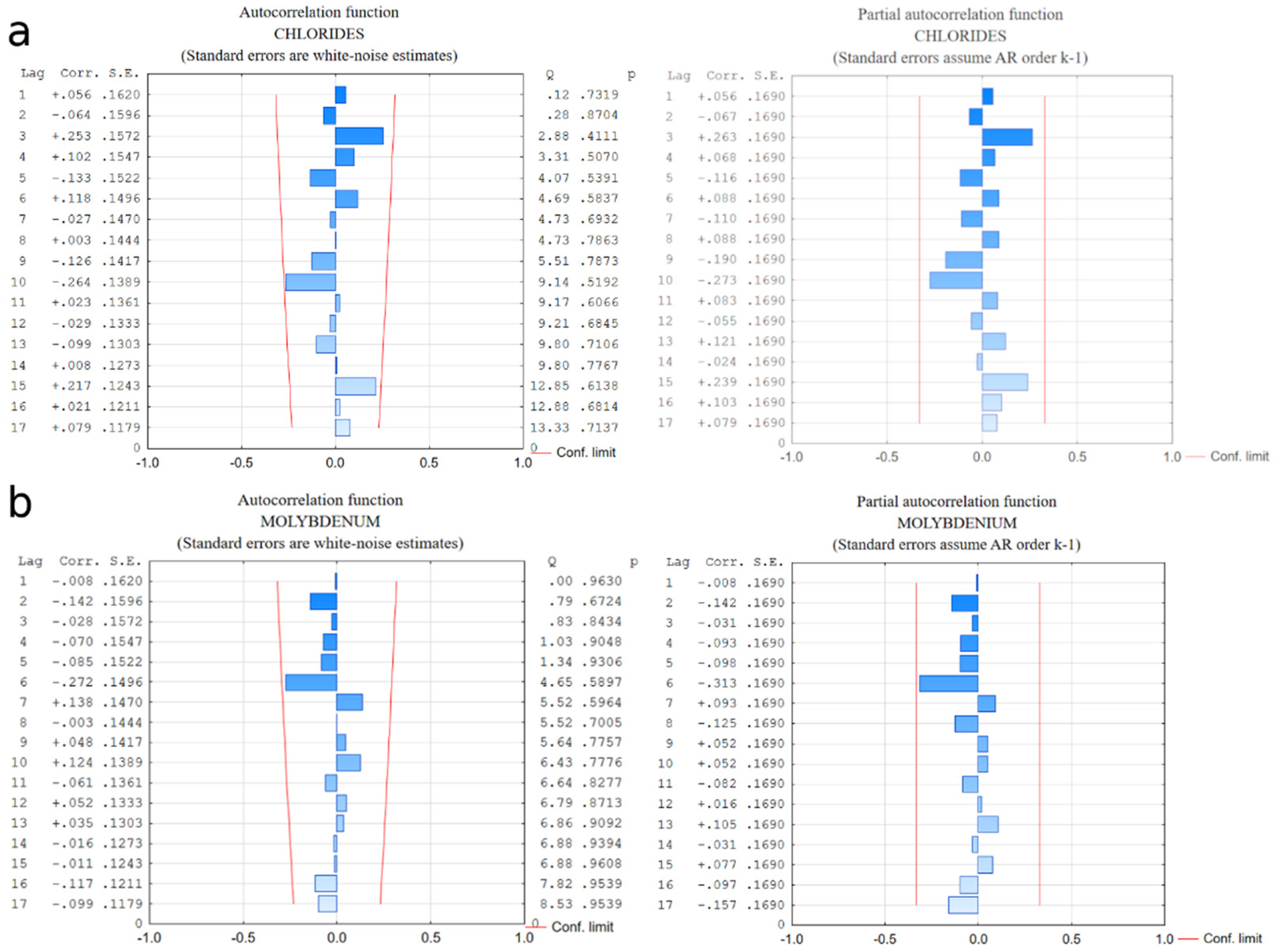
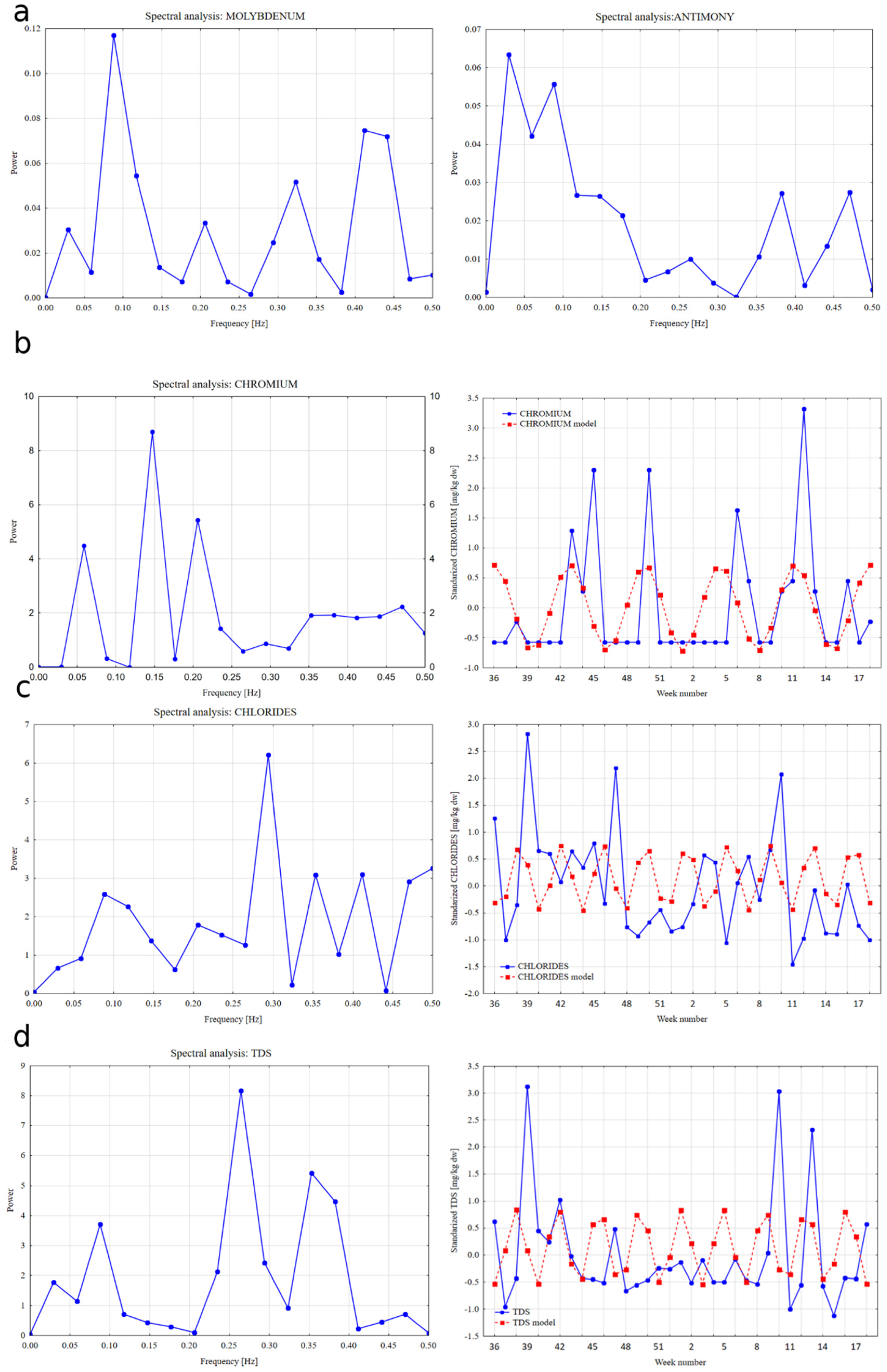
The occurrence of a single result outside the main control limits is the so-called point signal, while the location of two or more results outside the warning limits is referred to as the sequential signal [39]. In general, according to the principles of a normal distribution, approximately 4% of the results may fall outside the +/− 3 limits. These results can be removed from further analysis (e.g., trend analysis) or, if it is decided that it is not an error but simply the actual variability in the process, they can be taken for further analysis.
Trend analysis was performed using GWSDAT software (Ground Water Spatiotemporal Data Analysis Tool) [40]. In this program, trend analysis was performed using a nonparametric method called local linear regression. A traditional linear time series trend is estimated with a 95% confidence interval. The trend evaluation using the linear regression method is based on the assumption that if there is a trend in the analyzed data set, the directional coefficient of the line in the regression equation is different from zero. The sign of inclination (upward or downward trend) is indicated by the sign before the coefficient. If the value of the directional coefficient is not statistically significant, then we can conclude, that for the analyzed parameter no statistically significant monotonic trend has been identified. GWSDAT uses Mann-Kendall trend test to estimate the statistical significances of trends. The p-value below 0.05 indicates that the trend is statistically significant. In turn, a p-value above 0.05 suggests that the trend is not present.

2.2. Time Series

A time series is a series of data observations indexed in time order. The key characteristic features of time series are the trend and seasonality components. Therefore, a strong emphasis should be placed on seasonality and trend analysis. Trend analysis should be performed using ARIMA models, exponential smoothing, regression methods, Census I, Census II, and Tramo-Seat methods. The most popular seasonality analysis methods are Census I, Census II, ACF, and frequency analysis. The selection of appropriate methods depends on many factors, for example: the number of observations and seasons, trend type, and the strength of an irregular component.
Seasonality analysis was performed using the autocorrelation function (ACF), the partial autocorrelation function (PACF), and the frequency analysis.
The autocorrelation functions describe the relationships between delays in time series. The autocorrelation function (ACF) is expressed as a series of Pearson’s correlation coefficients for each lag in time series [41]. The partial autocorrelation function (PACF) is similar to the ACF. PACF is the partial correlation of a time series with its own lagged values and regressed values of the time series at all shorter lags [42].
The last method used for seasonality analysis was spectral analysis with Fast Fourier transform (FFT). The Fourier transform is a mathematical tool used to convert time series from the domain of time to the domain of frequency. During the analysis, the data are decomposed into a group of sine and cosine functions [43]. Time series can be expressed as a sum of harmonic frequencies (1):
x t = j = 1 n / 2 [ β 1 ( j n ) cos ( 2 π ω j t ) + β 2 ( j n ) sin ( 2 π ω j t ) ]
where:
  • β j —sine and cosine coefficients;
  • ω j —frequency; and
  • t—time (from 0 to n).
The most valuable harmonic frequencies can be identified using periodogram analysis, expressed as [44] (2):
P ( j n ) = β 1 2 ( j n ) + β 2 2 ( j n )
The Census I, Census II, and Tramo-Seat methods cannot be performed due to the limited amount of data. The analysis in the frequency domain and the model based on the Fourier transform were used with time domain analysis, autocorrelation function (ACF), and partial autocorrelation function (PACF). The determined seasonality requires additional statistical analysis of individual seasons, with box and whisker plots and ANOVA analysis.

3. Results

3.1. Control Charts and Trend Analysis

The obtained analytical data on the leachability of individual elements and chemical compounds were the basis for further analysis.
In general, most of the unprocessed IBA are extremely heterogeneous and have varied chemical composition. IBA are mainly composed of amorphous substances and minerals rich in calcium and silicates and are enriched with iron and sodium [45,46,47]. The main mineral components of municipal IBA are quartz, gehlenite, calcite, lime, and minerals from the spinel group (e.g., magnetite: Fe3O4). They also include metal oxides, sulfates, and carbonates [47]. The elements that constitute a potential source of pollution occur in the form of oxides or are associated with aluminosilicates [48]. Cu, Zn, Pb, and chlorides, which are found in significant quantities in IBA, are particularly dangerous [49]. Furthermore, IBA from MSW also contain fragments of glass, ceramic, and various types of metals, which are usually separated in separators.
When determining the leachability, the content of certain elements was below the detection threshold; therefore, their statistical analysis was abandoned. During the analysis of the control charts, the leachability of arsenic, cadmium, mercury, nickel, selenium, and fluorides was completely omitted. In the case of chromium, lead, and zinc, the limit of determination was considered as their concentration.
Figure 1, Figure 2 and Figure 3 show the control charts and trend analysis for the leachability of elements and compounds from the IBA. Using the control chart and the permissible values of individual leachability components plotted on the graph, it was possible to determine whether the deviation from the set standard found at a given moment could be treated as a random deviation or as a special deviation that could not be explained by the action of random factors. If the control chart signals a special deviation from the prescribed standard, a signal that the process is out of control is emitted. This is the first step in a series of efforts to detect and eliminate the real cause of process deregulation. During the test, one sample (concentration above the upper range of analytical method—10/mg/kg) with exceeded leachability limit values (LLVs) (10 mg/kg standard) was detected (Figure 2a). Based on the analysis of the chart, it was assumed that the result was random and most likely caused by an analytical error. Re-examination of the sample confirmed that the permissible leachability limit was not exceeded (concentration below the limit of quantification 0.1 mg/kg). The source of lead in IBA is, among others, lead chlorides, wulfenite, or anglesite [50]. The average concentration of lead leached over the 34-week period was 0.85 mg/kg (Table 2). However, the variability in the content of this component was high. The control charts also contain the leachability limit values for processing outside the plant using the R5 recovery process (LLVR5). The presented control charts clearly show outliers, which should be thoroughly verified. The amount of lead leached from IBA is highly variable. In some samples, the lead content was at the limits of detection, and in some cases exceeded the LLVR5 limit. In the initial period of observation, two samples with outliers were recorded. The analysis did not reveal any trend (Mann–Kendall test significance above 0.05) in the leachability of lead from IBA. According to many studies, lead concentration depends on many factors, especially pH, and also on the solubility of lead compounds, such as hydrocer-rusite (Pb3(CO3)2(OH)2) and cerrusite (PbCO3) [16]. Furthermore, the amount of lead in the waste is highly variable, as indicated by studies performed in Japan [51], Germany [52], Italy [53], or Lithuania [54], where the lead content exceeded 4500 mg/kg [53]. The analysis carried out on bottom ash from the MSA incinerator in Klaipeda showed that the concentration of lead in the leaching process was in the range of 0.2–12.2 mg [54]. In addition, the analysis of municipal solid waste incineration bottom ash from Macao showed that lead (Pb) concentrations reached as high as 19.6 mg/kg, far exceeding the maximum concentration limit [55].
In the tested IBA, the average leachability of barium was 9.66 mg/kg. The barium in IBA is most often found in the form of barite and barium oxides [56]. The highest barium leachability was observed in the initial observation period, where one outlier was 80.6 mg/kg with a maximum LLV of 100 mg/kg. On the basis of the control charts, it was also found that the LLVR5 was exceeded. The trend analysis showed a slight downward trend in barium content, which is certainly related to high measurement values in the initial period of obtaining results (Figure 1a, Table 2).
Copper in IBA, like other metals, is bound to non-silicate minerals [51]. It also occurs in the form of sulfates and spinels, e.g., with iron [52]. The content of leached copper was a maximum of 1.05 mg/kg and did not exceed the LLV (50 mg/kg); however, in the case of the two tested samples, it was higher than the LLVR5 (0.9) (Figure 1b, Table 2). In the case of copper leaching, one sequential signal was also recorded. No trend for the leachability of copper was found, but its variability over the period considered was high. Such a high variability is due to the high variability of the copper content in the combustion waste and in the bottom ash itself. Furthermore, the copper content in bottom ash from various installations is also highly variable and ranges from 1100 to 7700 mg/kg [54].
The leachability of chromium from IBA is moderately varied. In some samples, the amount of leachable chromium is lower than the detection limit, and in five cases, it was higher than LLVR5 (0.2 mg/kg), reaching a maximum of 0.33 mg/ kg (Table 2, Figure 1c). One sequential signal was also observed on the chromium control charts; no trend was detected.
Molybdenum in leached sediments occurred in concentrations from <0.1 to 0.71 mg/kg. However, all the obtained results were below LLV (10mg/kg). Eleven samples from different periods had values higher than MLR5 (0.3 mg/kg) and one sample can be defined as an outlier (Table 2, Figure 1d). The trend analysis did not reveal any trends in the amount of molybdenum leached.
The leachability of antimony from the IBA tested in most cases exceeds LLVR5 (0.02mg/kg). The variability of the antimony content is relatively high, ranging from 0.01 to 0.42mg/kg (Table 2, Figure 2b). There was also no trend for the antimony content. The zinc content of the leached solution was low in most samples. However, in some samples, the amounts of zinc were defined as outliers and the LLVR5 (2 mg/kg) was exceeded. The maximum content of leached zinc in the tested samples was 8.85 mg/kg; the zinc content was very high (Table 2, Figure 2c). According to the study on leaching of Cu, Zn, Pb, and Cd from bottom ash by Tang and Steenari [57], this process is influenced by many factors, especially pH, temperature, time, and liquid/solid ratio, but also by the chemical and physical nature of the ash. Local factors, such as the composition of the waste used as fuel in the incinerator and the technical characteristics of the combustion chamber and the particle separation equipment used, also have a significant influence on the chemical properties of the ash generated.
Chlorides are one of the most troublesome compounds leached from IBA. The LLV for this component is 15,000 mg/kg. The chloride content ranges from 871 to 4010 mg/kg. In all tested IBA samples, the chloride content was above LLVR5 (Table 2, Figure 2d). The trend analysis showed a downward trend for the leachability of chloride from IBA.
The leachability of sulfates from the IBA tested is highly variable and ranges from 50 to 2990 mg/kg (Table 2, Figure 3a). These contents do not exceed the LLV of 20,000 mg /kg, though the LLVR5 was exceeded many times. The control chart also shows two outliers, suggesting that the IBA composition is unstable. This instability and high variability of sulfate leaching from IBA is also confirmed by the lack of a trend.
For comparison, the amount of compounds leached from bottom ash from the incineration plant in Kraków is much lower than in the case of the Klaipeda incinerator. Leaching studies showed that large amounts of soluble salts were leached from IBA from the Klaipeda incinerator, mainly sulphates (2816–10,012 mg/kg), chlorides (1869–3046 mg/kg), and some heavy metals (Mo 0.5–1.8 mg/kg, Pb 0.1–2.5 mg/kg) [58].
The dissolved organic carbon (DOC) content of the leached sludge is moderately variable. It ranges from 22.40 to 124 mg/kg, with a maximum LLV of 800 mg/kg and an LLVR5 of 240 mg/kg (Table 2, Figure 3b). During the first observation, one outlier was recorded. However, the analysis showed no trend.
The amount of leached total dissolved substances (TDS) from IBA was moderately variable during the analyzed period and ranged from 5200 to 23,400 mg/kg. The leachability of TDS was greater than the LLVR5 (2500 mg/kg) in all of the tested samples but did not exceed the LLV (60,000 mg/kg). The analysis showed no trend and one outlier was recorded on the control charts (Table 2, Figure 3c).

3.2. Assessment of Seasonality and Trend

In the further part of the analysis, time series analysis was used to assess the seasonality and trend in the leaching of individual components from the tested IBA samples.
Values lower (or higher in the case of lead) than the limits shown were changed to limit values. One of the samples did not meet the LLV (two measurements in the same week) and was excluded from the analysis. The sample no. 3.1 can be defined as an outlier for some of the analyzed elements and as an extreme value for lead. This sample was excluded from further analysis. Because of the fact that the tested samples showed low concentrations, below the detection limit, which meant that the obtained results were constant, the analysis of the time series for arsenic, cadmium, mercury, nickel, selenium, and fluoride was abandoned.
The seasonality and trend analyses were performed on the basis of autocorrelation (ACF) and partial autocorrelation (PACF) plots. The obtained results are shown in Figure 4 and Figure 5. Based on the statistically significant correlations on the chart and the shape of the chart, it can be determined whether there is a trend and/or periodicity in the data. The maximum time lag for the autocorrelations is half of the observations.
Analysis of the seasonality using ACF and PACF shows the lack of trend and seasonality in copper, dry mass, lead, sulfates, and zinc. The correlation values for the individual lags are low and do not exceed the confidence levels.
For some elements and chemical compounds, the ACF (Figure 4) and PACF (Figure 4) plots contain individual correlations at the confidence limit. Because of the low number of observations, there is a need for further analysis carried out in line with the methodology for data with a trend or seasonality. This group includes chlorides (lag 10: R = −0.26; lag 15: R = 0.21) and molybdenum (lag 6: R = −0.27) (Figure 4).
The last group included elements and chemical compounds for which some lags show statistically significant correlations. These include antimony, barium, chromium, and TDS.
The barium ACF plot shows the first five lags with statistically significant correlations and the first leading lag in the PACF plot (Figure 5a). This indicates a trend in the non-linear data. This trend can be described by the following formula:
BARIUM = 30.3728 − 2.0594 ∗ x + 0.0382 ∗ x2
For barium, a second-degree polynomial or some other fast-fading function seems to be a suitable match. From week 43, barium stabilizes at a similar level with little variation.
The ACF plot for chromium shows a statistically significant correlation for delay 14 (R = 0.29); in the case of the PACF plot, the delay 14 is not statistically significant (Figure 5b).
The leachability of antimony shows the first ACF lags at the border of statistical significance (lag 1: R = 0.32, lag 2: R = 0.30) with no statistically significant correlation for the 1 delay for PACF. The time lag 9 is statistically significant with R = 0.32 (Figure 5c).
For TDS, the maximum statistically significant correlation was observed for the lag 3 (R = 0.34) and the correlation for the PACF for this lag is 0.32 and is at the border of statistical significance (Figure 5d).
For further seasonality analysis, the following variables were selected: chromium, molybdenum, antimony, chlorides, and TDS.
Then, the frequency estimation was performed. The ACF and PACF were constructed to check the seasonality and trend occurrence (Figure 6). In order to accurately assess the seasonality, analysis in the frequency domain was performed. The frequency analysis was based on the fast Fourier transform (FFT) and periodogram. The statistically significant frequencies for α = 0.05 should be higher than approximately 1.5. The analysis did not confirm the seasonality for antimony and molybdenum; periodogram values for any frequencies were not statistically significant (α = 0.05). For molybdenum and antimony, the highest periodogram value was recorded for the frequency corresponding to 11 weeks and the periodogram values are not statistically significant (Figure 6b). Therefore, the seasonality was not confirmed.
In the FFT analysis of chromium, the highest frequency of 0.147 corresponds to the period of 7 weeks, and the value of the periodogram is statistically significant (α = 0.05, power 8.7). The frequency analysis confirmed the existence of seasonality. Therefore, the results of Fourier’s analysis (period 7 weeks) are not compatible with ACF and PACF (period of 14 weeks). To finally exclude or confirm seasonality, a model for the frequency of 0.15 was developed. The use of Fourier analysis to confirm the seasonality was also necessary in the case of leachability of chlorides and TDS. In the case of chlorides, the maximum statistically significant values were found for the period of 3 and 4 weeks, which means that the obtained results are not compatible with the ACF and PACF analysis. For TDS, the maximum periodogram value occurred for period 4. The ACF and PACF plots indicate the lag 3 and the periodogram values are statistically significant. Such results may be due to the spectral leakage to adjacent frequencies.
The model for the frequency with the highest periodogram values created for chromium, chlorides, and TDS was compared with the real data. In addition, box and whisker plots were created (Figure 7).
The Fourier model for the leached chromium at the frequency 0.147059 gave a 7-week period. This is significantly different from the result obtained using ACF and PCF (10 weeks). Model quality evaluated with the determination coefficient (R2) equals 0.073. It shows insufficient fitting between the model and chromium data. The Fourier model for chlorides and TDS at a frequency of 0.26470 gave a 4-week period. The model quality is also insufficient with R2 lower than 0.1.
For chromium, chloride, and TDS, a statistical analysis of the seasons using box and whisker plots was also performed (Figure 7). Original data were divided into seasons based on periodogram values. Basic descriptive statistics, mean and standard deviation, were computed for each season and presented in the plot. The average values for individual seasons for chloride are similar, seasonal variation is not visible in the box and whisker plot. The same lack of variance between seasons is visible in the TDS data. Based on the charts, we can say that there is no statistically significant difference between the seasons.
In the case of chromium, differences in the average level of the phenomenon can be noticed. For this reason, a one-way analysis of variance (abbreviated one-way ANOVA) was performed.
The ANOVA results for chromium are statistically significant: F(6,28) = 2.47, p < 0.048. It shows that at least one group differs significantly from the others. To determine which one, post-hoc tests are required. Post-hoc Scheffe and least significant differences (LSD) tests were conducted. The most rigorous Scheffe’s test does not confirm a statistically significant difference in the mean values for individual groups; however, in the case of the less stringent LSD test, the season defined as 2 differs significantly from the others. Season 2 differs from 1, 5, 6, and 0 subsequently with p values of 0.017, 0.005, 0.013, and 0.011.

4. Conclusions

The analysis of the leachability of elements and compounds from IBA is one of the key factors in determining their use. As can be seen for all the elements tested, in some samples, the content of leached elements is higher than the leachability limit values for processing outside the installation using the R5 recovery process (LLVR5). In the case of leaching of barium and chloride from IBA, a downward trend was demonstrated based on the GWSDAT analysis. A similar trend was shown for barium leaching using the ACF and PACF analysis. Barium differed from the other elements and compounds; the first lag with statistically significant correlation provided trend existence, also confirmed by the line graph. In the case of barium, a polynomial trend can be used; however, after an initial decrease in the average level of the phenomenon, the data remains stable.
In other cases, the trend analysis did not show any regularities. Based on the obtained results, it can be stated that most elements and compounds are random, and no seasonality was observed. ACF and PACF graphs show statistically significant correlations for lags (with lag and correlation sign) in barium (1 positive), chromium (14 positive), antimony (9 negative), and TDS (3 positive). For chlorides, the molybdenum correlation for one lag was on the border of statistical significance (lag and correlation sign: 10 positive, 6 negative). For the leaching of chromium, chloride, and TDS, a Fourier model and statistical analysis of the seasons were performed to confirm or exclude the occurrence of seasonality in the data. Despite statistically significant periodogram values for TDS, the frequency of 0.264 is weak.
Furthermore, a box and whisker plot and a one-way analysis of variance (ANOVA) did not confirm the existence of differences between seasons. The same results were obtained for chlorides. The ANOVA analysis showed that in the case of chromium, at least one group differs significantly from the rest, but the Scheffe’s test did not confirm the test result. The result of the NIR test was not confirmed by the rest of the obtained results for chromium. Hence, it can be concluded that also for chromium the seasonality was not observed.
The only element that shows seasonality (very weak and visually poorly matched) is chromium. In the case of chromium, the seasonality cannot be ruled out on the basis of analysis. However, based on borderline significance, this is likely to be a random event associated with a small number of observations.
The analysis of control charts and time series showed that the chemical composition and leachability of selected elements and compounds was stable. However, the exceedances of the LLVR5 meant that the use of IBA in the recovery in the R5 process as required in [25], following an initial weathering period of two weeks, was limited. Other studies have shown the intensity of the leaching process decreases when the wastes are subjected to accelerated carbonation [59] or weathering [60]. Meima et al. [61] determined three stages of natural weathering/carbonation. Every single stage has its own pH range between 8 and 8.5, where calcite is formed and dominant, and trace elements are trapped into carbonates [62], with the major heavy metal content in grain size fraction below 2 mm [7]. Reported studies indicate that the leaching process stabilizes as the weathering time increases. The issue requires further analysis in ZTPO and evaluation of the impact of the IBA weathering time on the leachability of elements and substances contained in them.
The research methodology, which was presented on the example of the leachability of elements and compounds from IBA, can also be used for other waste analyses. However, the main limitation of the application of the presented method is the representativeness of the tested samples, which was clearly visible in the case of lead. In one case, the lead content significantly differed from the other results. However, after repeating the analysis, the obtained values were correct. Therefore, the sample collection and averaging are crucial, as this affects the results of the statistical analysis.

Author Contributions

Conceptualization, B.B. and R.J.; methodology, K.W. and M.C.; data curation, B.B., R.J., M.C. and K.W.; writing—original draft preparation, B.B.; writing—review and editing, R.J.; visualization, K.W. and M.C. All authors have read and agreed to the published version of the manuscript.

Funding

This research was funded by the Ministry of Science and Higher Education (subsidy No. 16.16.140.315).

Institutional Review Board Statement

Not applicable.

Informed Consent Statement

Not applicable.

Conflicts of Interest

The authors declare no conflict of interest.

References

  1. Alba, N.; Gassó, S.; Lacorte, T.; Baldasano, J.M. Characterization of municipal solid waste incineration residues from facilities with different air pollution control systems. J. Air Waste Manag. Assoc. 1997, 47, 1170–1179. [Google Scholar] [CrossRef]
  2. European Commission. Council Directive 1999/31/EC of 26 April 1999 on the Landfill of Waste; European Commission: Luxembourg, 1999. [Google Scholar]
  3. European Commission. Directive 2008/98/EC of the European Parliament and of the Council of 19 November 2008 on waste and repealing certain Directives. Off. J. Eur. Union 2008, 51, 47. [Google Scholar]
  4. Ministerstwo Środowiska. Rozporządzenie Ministra Gospodarki z Dnia 16 Lipca 2015 r. w Sprawie Dopuszczania Odpadów do Składowania na Składowiskach, Dz.U. 2015 poz. 1277; Ministerstwo Środowiska: Warsaw, Poland, 2015.
  5. Sabbas, T.; Polettini, A.; Pomi, R.; Astrup, T.; Hjelmar, O.; Mostbauer, P.; Cappai, G.; Magel, G.; Salhofer, S.; Speiser, C.; et al. Management of municipal solid waste incineration residues. Waste Manag. 2003, 23, 61–88. [Google Scholar] [CrossRef]
  6. Jung, C.H.; Matsuto, T.; Tanaka, N.; Okada, T. Metal distribution in incineration residues of municipal solid waste (MSW) in Japan. Waste Manag. 2004, 24, 381–391. [Google Scholar] [CrossRef] [Green Version]
  7. Abramov, S.; He, J.; Wimmer, D.; Lemloh, M.L.; Muehe, E.M.; Gann, B.; Roehm, E.; Kirchhof, R.; Babechuk, M.G.; Schoenberg, R.; et al. Heavy metal mobility and valuable contents of processed municipal solid waste incineration residues from Southwestern Germany. Waste Manag. 2018, 79, 735–743. [Google Scholar] [CrossRef]
  8. Yao, Q.; Samad, N.B.; Keller, B.; Seah, X.S.; Huang, L.; Lau, R. Mobility of heavy metals and rare earth elements in incineration bottom ash through particle size reduction. Chem. Eng. Sci. 2014, 118, 214–220. [Google Scholar] [CrossRef]
  9. Šyc, M.; Simon, F.G.; Hykš, J.; Braga, R.; Biganzoli, L.; Costa, G.; Funari, V.; Grosso, M. Metal recovery from incineration bottom ash: State-of-the-art and recent developments. J. Hazard. Mater. 2020, 393, 122433. [Google Scholar] [CrossRef]
  10. Forteza, R.; Far, M.; Seguí, C.; Cerdá, V. Characterization of bottom ash in municipal solid waste incinerators for its use in road base. Waste Manag. 2004, 24, 899–909. [Google Scholar] [CrossRef]
  11. Blasenbauer, D.; Huber, F.; Lederer, J.; Quina, M.J.; Blanc-Biscarat, D.; Bogush, A.; Bontempi, E.; Blondeau, J.; Chimenos, J.M.; Dahlbo, H.; et al. Legal situation and current practice of waste incineration bottom ash utilisation in Europe. Waste Manag. 2020, 102, 868–883. [Google Scholar] [CrossRef]
  12. Lynn, C.J.; OBE, R.K.; Ghataora, G.S. Municipal incinerated bottom ash characteristics and potential for use as aggregate in concrete. Constr. Build. Mater. 2016, 127, 504–517. [Google Scholar] [CrossRef]
  13. Van Dr Wegen, G.; Hofstra, U.; Speerstra, J. Upgraded MSWI bottom ash as aggregate in concrete. Waste Biomass Valorization 2013, 4, 737–743. [Google Scholar] [CrossRef]
  14. Yin, K.; Chan, W.P.; Dou, X.; Ren, F.; Wei-Chung Chang, V. Cr, Cu, Hg and Ni release from incineration bottom ash during utilization in land reclamation—based on lab-scale batch and column leaching experiments and a modeling study. Chemosphere 2018, 197, 741–748. [Google Scholar] [CrossRef] [PubMed]
  15. Kim, S.Y.; Tanaka, N.; Matsuto, T. Solubility and adsorption characteristics of Pb in leachate from MSW incinerator bottom ash. Waste Manag. Res. 2002, 20, 373–381. [Google Scholar] [CrossRef] [PubMed] [Green Version]
  16. Dijkstra, J.J.; Van Der Sloot, H.A.; Comans, R.N.J. The leaching of major and trace elements from MSWI bottom ash as a function of pH and time. Appl. Geochem. 2006, 21, 335–351. [Google Scholar] [CrossRef]
  17. Van Der Sloot, H.A.; Kosson, D.S.; Hjelmar, O. Characteristics, treatment and utilization of residues from municipal waste incineration. Waste Manag. 2001, 21, 753–765. [Google Scholar] [CrossRef]
  18. Vateva, I.; Laner, D. Grain-size specific characterisation and resource potentials of municipal solid waste incineration (MSWI) bottom ash: A German case study. Resources 2020, 9, 66. [Google Scholar] [CrossRef]
  19. Caviglia, C.; Confalonieri, G.; Corazzari, I.; Destefanis, E.; Mandrone, G.; Pastero, L.; Boero, R.; Pavese, A. Effects of particle size on properties and thermal inertization of bottom ashes (MSW of Turin’s incinerator). Waste Manag. 2019, 84, 340–354. [Google Scholar] [CrossRef]
  20. Del Valle-Zermeño, R.; Gómez-Manrique, J.; Giro-Paloma, J.; Formosa, J.; Chimenos, J.M. Material characterization of the MSWI bottom ash as a function of particle size. Effects of glass recycling over time. Sci. Total Environ. 2017, 581–582, 897–905. [Google Scholar] [CrossRef] [Green Version]
  21. Loginova, E.; Volkov, D.S.; van de Wouw, P.M.F.; Florea, M.V.A.; Brouwers, H.J.H. Detailed characterization of particle size fractions of municipal solid waste incineration bottom ash. J. Clean. Prod. 2019, 207, 866–874. [Google Scholar] [CrossRef]
  22. Huber, F.; Blasenbauer, D.; Aschenbrenner, P.; Fellner, J. Complete determination of the material composition of municipal solid waste incineration bottom ash. Waste Manag. 2020, 102, 677–685. [Google Scholar] [CrossRef]
  23. Hyks, J.; Astrup, T.; Christensen, T.H. Long-term leaching from MSWI air-pollution-control residues: Leaching characterization and modeling. J. Hazard. Mater. 2009, 162, 80–91. [Google Scholar] [CrossRef] [PubMed]
  24. European Commission. 2000/532/EC, COMMISSION DECISION of 3 May 2000 Replacing Decision 94/3/EC Establishing a List of Wastes Pursuant to Article 1(a) of Council Directive 75/442/EEC on Waste and Council Decision 94/904/EC Establishing a List of Hazardous Waste Pursuant to Art; European Commission: Luxembourg, 2020. [Google Scholar]
  25. Ministerstwo Środowiska. Rozporządzenie Ministra Środowiska z Dnia 11 Maja 2015 r. w Sprawie Odzysku Odpadów Poza Instalacjami i Urządzeniami. Dz.U. 2015 poz. 796; Ministerstwo Środowiska: Warsaw, Poland, 2015.
  26. EN 12457-1:2002. Characterisation of Waste—Leaching—Compliance Test for Leaching of Granular Waste Materials and Sludges—Part 1: One Stage Batch Test at a Liquid to Solid Ratio of 2 L/kg for Materials with High Solid Content and with Particle Size Below 4 mm; European Standards: Brussels, Belgium, 2002. [Google Scholar]
  27. EN 12457-2. Characterisation of Waste LEACHING Compliance Test for Leaching of Granular Waste Materials and Sludges Part 2: One Stage Batch Test at a Liquid to Solid Ratio of 10 L/kg for Materials with Particle Size Below 4 mm (without or with Size Reduction); European Standards: Brussels, Belgium, 2002. [Google Scholar]
  28. EN 12457-3. Characterisation of Waste. Leaching. Compliance Test for Leaching of Granular Waste Materials and Sludges. Two Stage batch Test at a Liquid to Solid Ratio of 2 L/kg and 8 L/kg for Materials with a High Solid Content and with a Particle Size Below 4 mm (without or with Size Reduction); European Standards: Brussels, Belgium, 2002. [Google Scholar]
  29. EN 12457-4. Characterisation of Waste. Leaching. Compliance Test for Leaching of Granular Waste Materials and Sludges. One Stage Batch Test at a Liquid to Solid Ratio of 10 L/kg for Materials with Particle Size Below 10 mm (without or with size reduction); European Standards: Brussels, Belgium, 2002. [Google Scholar]
  30. ISO/IEC 17025:2017. General Requirements for the Competence of Testing and Calibration Laboratories; ISO: Geneva, Switzerland, 2017. [Google Scholar]
  31. UNE. EN 15934:2012. Sludge, Treated Biowaste, Soil and Waste—Calculation of Dry Matter Fraction after Determination of Dry Residue or Water Content (Endorsed by AENOR in October of 2012); European Standards: Brussels, Belgium, 2012. [Google Scholar]
  32. ISO. ISO 17294-2:2016. Water Quality—Application of Inductively Coupled Plasma Mass Spectrometry (ICP-MS)—Part 2: Determination of Selected Elements Including Uranium Isotopes; ISO: Geneva, Switzerland, 2016. [Google Scholar]
  33. ISO. ISO 12846:2012. Water Quality—Determination of Mercury—Method Using Atomic Absorption Spectrometry (AAS) with and without Enrichment; ISO: Geneva, Switzerland, 2012. [Google Scholar]
  34. ISO. ISO 15682:2000. Water Quality—Determination of Chloride by Flow Analysis (CFA and FIA) and Photometric or Potentiometric Detection; ISO: Geneva, Switzerland, 2000. [Google Scholar]
  35. ISO. ISO 22743:2006. Water Quality—Determination of Sulfates—Method by Continuous Flow Analysis (CFA); ISO: Geneva, Switzerland, 2006. [Google Scholar]
  36. ISO. ISO/TS 17951-2:2016. Water Quality—Determination of Fluoride Using Flow Analysis (FIA and CFA)—Part 2: Method Using Continuous Flow Analysis (CFA) with Automated In-line Distillation; ISO: Geneva, Switzerland, 2016. [Google Scholar]
  37. BS EN 1484:1997. Water Analysis. Guidelines for the Determination of Total Organic Carbon (TOC) and Dissolved Organic Carbon (DOC); European Standards: Brussels, Belgium, 1997. [Google Scholar]
  38. NEMI Method Summary—2540 C. Available online: https://www.nemi.gov/methods/method_summary/9818/ (accessed on 14 January 2021).
  39. Massart, D.L.; Vandeginste, B.G.M.; Buydens, L.M.C.; de Jong, S.; Lewi, P.J.; Smeyers-Verbeke, J. Handbook of Chemometrics and Qualimetrics: Part A; Data Handling in Science and Technology Volume 20A; Elsevier: Amsterdam, The Netherlands, 1997; p. Xvii. ISBN 0-444-89724-0. [Google Scholar]
  40. Jones, W.; Spence, M. GroundWater Spatio-Temporal Data Analysis Tool (GWSDAT Version 2.0) User Manual; Shell Global Solutions: Manchester, UK, 2013. [Google Scholar]
  41. Chatfield, C. The Analysis of Time Series: An Introduction, 6th ed.; Chapman & Hall/CRC: Boca Raton, FL, USA, 2004. [Google Scholar]
  42. Ramsey, F.L. Characterization of the Partial Autocorrelation Function. Ann. Stat. 1974, 2, 1296–1301. [Google Scholar] [CrossRef]
  43. Shumway, R.H.; Stoffer, D.S. Time Series Analysis and Its Applications: With R Examples; Springer: Berlin/Heidelberg, Germany, 2009. [Google Scholar]
  44. Bloomfield, P. Fourier Analysis of Time Series; Wiley Series in Probability and Statistics; John Wiley & Sons, Inc.: Hoboken, NJ, USA, 2000; Volume 22, ISBN 9780471722236. [Google Scholar]
  45. Kowalski, P.; Michalik, M. Slags and Ashes from Municipal Waste Incineration in Poland-Mineralogical and Chemical Composition. Geophys. Res. Abstr. 2013, 15, 12642. [Google Scholar]
  46. Eusden, J.D.; Eighmy, T.T.; Hockert, K.; Holland, E.; Marsella, K. Petrogenesis of municipal solid waste combustion bottom ash. Appl. Geochem. 1999, 14, 1073–1091. [Google Scholar] [CrossRef]
  47. Zevenbergen, C.; Vander Wood, T.; Bradley, J.P.; Van der Broeck, P.F.C.W.; Orbons, A.J.; Van Reeuwijk, L.P. Morphological and chemical properties of MSWI bottom ash with respect to the glassy constituents. Hazard. Waste Hazard. Mater. 1994, 11, 371–383. [Google Scholar] [CrossRef]
  48. Chang, F.Y.; Wey, M.Y. Comparison of the characteristics of bottom and fly ashes generated from various incineration processes. J. Hazard. Mater. 2006, 138, 594–603. [Google Scholar] [CrossRef]
  49. Kowalski, P.R.; Kasina, M.; Michalik, M. Metallic Elements Fractionation in Municipal Solid Waste Incineration Residues. Energy Procedia 2016, 97, 31–36. [Google Scholar] [CrossRef] [Green Version]
  50. Krzanowski, J.E.; Crannell, B.S.; Krzanowski, J.E.; Eighmy, T.T.; Crannell, B.S.; Dykstra Eusden, J.; Eusden, J.D. An analytical electron microscopy investigation of municipal solid waste incineration bottom ash. J. Mater. Res. 1998, 13, 28–36. [Google Scholar] [CrossRef]
  51. Wei, Y.; Shimaoka, T.; Saffarzadeh, A.; Takahashi, F. Mineralogical characterization of municipal solid waste incineration bottom ash with an emphasis on heavy metal-bearing phases. J. Hazard. Mater. 2011, 187, 534–543. [Google Scholar] [CrossRef]
  52. Bayuseno, A.P.; Schmahl, W.W. Understanding the chemical and mineralogical properties of the inorganic portion of MSWI bottom ash. Waste Manag. 2010, 30, 1509–1520. [Google Scholar] [CrossRef]
  53. Rambaldi, E.; Esposito, L.; Andreola, F.; Barbieri, L.; Lancellotti, I.; Vassura, I. The recycling of MSWI bottom ash in silicate based ceramic. Ceram. Int. 2010, 36, 2469–2476. [Google Scholar] [CrossRef]
  54. Seniunaite, J.; Vasarevicius, S. Leaching of Copper, Lead and Zinc from Municipal Solid Waste Incineration Bottom Ash. In Energy Procedia; Elsevier Ltd.: Amsterdam, The Netherlands, 2017; Volume 113, pp. 442–449. [Google Scholar]
  55. Feng, S.; Wang, X.; Wei, G.; Peng, P.; Yang, Y.; Cao, Z. Leachates of municipal solid waste incineration bottom ash from Macao: Heavy metal concentrations and genotoxicity. Chemosphere 2007, 67, 1133–1137. [Google Scholar] [CrossRef]
  56. Stamps, B.W.; Lyles, C.N.; Suflita, J.M.; Masoner, J.R.; Cozzarelli, I.M.; Kolpin, D.W.; Stevenson, B.S. Municipal Solid Waste Landfills Harbor Distinct Microbiomes. Front. Microbiol. 2016, 7, 534. [Google Scholar] [CrossRef] [PubMed] [Green Version]
  57. Tang, J.; Steenari, B.M. Leaching optimization of municipal solid waste incineration ash for resource recovery: A case study of Cu, Zn, Pb and Cd. Waste Manag. 2016, 48, 315–322. [Google Scholar] [CrossRef] [PubMed]
  58. Seniūnaitė, J.; Vasarevičius, S.; Grubliauskas, R.; Zigmontienė, A.; Vaitkus, A. Characteristics of Bottom Ash from Municipal Solid Waste Incineration. Rocznik Ochrona Środowiska 2018, 20 Pt 1, 123–144. [Google Scholar]
  59. Santos, R.M.; Mertens, G.; Salman, M.; Cizer, Ö.; Van Gerven, T. Comparative study of ageing, heat treatment and accelerated carbonation for stabilization of municipal solid waste incineration bottom ash in view of reducing regulated heavy metal/metalloid leaching. J. Environ. Manag. 2013, 128, 807–821. [Google Scholar] [CrossRef] [Green Version]
  60. Meima, J.A.; Comans, R.N.J. The leaching of trace elements from municipal solid waste incinerator bottom ash at different stages of weathering. Appl. Geochem. 1999, 14, 159–171. [Google Scholar] [CrossRef]
  61. Meima, J.A.; Comans, R.N.J. Geochemical modeling of weathering reactions in municipal solid waste incinerator bottom ash. Environ. Sci. Technol. 1997, 31, 1269–1276. [Google Scholar] [CrossRef]
  62. Freyssinet, P.; Piantone, P.; Azaroual, M.; Itard, Y.; Clozel-Leloup, B.; Guyonnet, D.; Baubron, J.C. Chemical changes and leachate mass balance of municipal solid waste bottom ash submitted to weathering. Waste Manag. 2002, 22, 159–172. [Google Scholar] [CrossRef]
Figure 1. Control charts and trend analysis results for (a) Ba, (b) Cu, (c) Cr, and (d) Mo.
Energies 14 00771 g001
Figure 2. Control charts and trend analysis results for (a) Pb, (b) Sb, (c) Zn, and (d) Cl.
Energies 14 00771 g002
Figure 3. Control charts and trend analysis results for (a) SO42−, (b) DOC, and (c) TDS.
Energies 14 00771 g003
Figure 4. Analysis of seasonality (ACF and PACF; chlorides, molybdenum).
Energies 14 00771 g004
Figure 5. Analysis of seasonality (ACF and PACF; barium, chromium, antimony, and TDS).
Energies 14 00771 g005
Figure 6. Analysis with fast Fourier transform (FFT) periodogram and frequency models (molybdenum, antimony, chlorides, TDS).
Energies 14 00771 g006
Figure 7. Box and whisker plot ((a) chlorides, (b) chromium, (c) TDS).
Energies 14 00771 g007
Table 1. Analytical methods used for selected elements and compounds determination.
Element/CompoundAnalytical MethodLimit of Quantification (LOQ)Uncertainty (U) * (%)
Dry massWeight method [31]0.10%25
AsInductively Coupled Plasma Mass Spectrometry ICP-MS [32]0.10 mg/kg35
Cd0.010 mg/kg35
Ba0.10 mg/kg35
Cu0.10 mg/kg35
Cr0.10 mg/kg35
Mo0.10 mg/kg35
Ni0.10 mg/kg35
Pb0.10 mg/kg35
Se0.010 mg/kg40
Sb0.010 mg/kg35
Zn0.50 mg/kg35
HgAtomic Absorption Spectrometry with the amalgamation technique [33]0.005 mg/kg35
ClContinuous flow analysis method (CFA) with
spectrophotometric detection [34]
25 mg/kg29
SO42−Continuous flow analysis method (CFA) with
spectrophotometric detection [35]
50 mg/kg29
FContinuous flow analysis method (CFA) with
spectrophotometric detection [36]
5 mg/kg29
TOCInfrared spectroscopy [37]1.0 mg/L29
TDSWeight method [38]3.0 mg/L29
* related expanded uncertainty, k = 2.95%.
Table 2. Mean values for the analyzed variables and the values of outliers (2out) and extreme (3out).
VariableMeanMedianMinMaxStd. Dev.The Coefficient of Variation“−2 Std. Dev.”“+2 Std. Dev.”“−3 Std. Dev.”“+3 Std. Dev.”LLVLLVR5
Barium9.582.480.6180.6017.17175.29−24.7643.92−41.961.1≤1007
Copper0.280.210.101.050.2381.97−0.180.73−0.410.96≤500.9
Chromium0.130.100.100.330.0643.660.020.25−0.040.31≤100.2
Molybdenum0.280.260.100.710.1345.430.020.53−0.100.65≤100.3
Lead0.850.100.1010.001.88216.20−2.904.60−4.776.48≤100.2
Antimony0.150.150.010.420.1071.49−0.060.36−0.160.47≤0.70.02
Zinc1.190.530.508.851.70141.77−2.204.59−3.906.28≤502
Chlorides19381815.00871.004010.0073538.204683407−2664142≤15,000550
Sulfates612430.0050.002990.00722114.31−8322055−15532776≤20,000560
DOC49.040.0022.40124.0026.352.79−3.6101.5−29.8127.8≤800240
TDS89617537.505200.0023,400.00335743.70224715,674−111019031≤60,0002500
Publisher’s Note: MDPI stays neutral with regard to jurisdictional claims in published maps and institutional affiliations.

