Modelling a Heaving Point-Absorber with a Closed-Loop Control System Using the DualSPHysics Code

Abstract

The present work addresses the need for an efficient, versatile, accurate and open-source numerical tool to be used during the design stage of wave energy converters (WECs). The device considered here is the heaving point-absorber developed and tested by Sandia National Laboratories. The smoothed particle hydrodynamics (SPH) method, as implemented in DualSPHysics, is proposed since its meshless approach presents some important advantages when simulating floating devices. The dynamics of the power take-off system are also modelled by coupling DualSPHysics with the multi-physics library Project Chrono. A satisfactory matching between experimental and numerical results is obtained for: (i) the heave response of the device when forced via its actuator; (ii) the vertical forces acting on the fixed device under regular waves and; (iii) the heave response of the WEC under the action of both regular waves and the actuator force. This proves the ability of the numerical approach proposed to simulate accurately the fluid–structure interaction along with the WEC’s closed-loop control system. In addition, radiation models built from the experimental and WAMIT results are compared with DualSPHysics by plotting the intrinsic impedance in the frequency domain, showing that the SPH method can be also employed for system identification.

1. Introduction

A wide variety of wave energy converter (WEC) designs are currently being developed, but very few are generating electricity commercially (see, e.g., [1,2]). According to the JRC Ocean Energy Status Report (2016 edition) [3], the highest percentage of research and development efforts have been focused on the technology of the point absorbers. These devices consist of a floating buoy whose oscillating motion, heaving and/or pitching, is converted into electricity by means of a power take-off (PTO) system. Modeling of these WECs should account for device kinematics, hydrodynamics, electromechanics, and closed-loop control systems. The incorporation of a control system is of particular importance since, in order to extract power in an efficient manner, the PTO unit must be controlled. Furthermore, a significant body of research has shown the benefits of applying more advanced control techniques [4,5].

A number of approaches are typically used to perform design analyses of point absorbers. Physical experiments are widely used and usually play a key role in concept exploration and model validation/identification. Some works focused on the wave tank testing of point-absorbers are [6,7,8,9]. Nevertheless, physical experiments have high costs associated with the construction, deployment and maintenance of the prototypes and facilities. This, along with the exponential growth of the computational resources in the last decades, has boosted the use of numerical methods during the design stages of WECs. Different reviews highlight the main advances of the numerical modelling of WECs achieved during the last decades [10,11,12,13,14]. Furthermore, ref. [15] reviewed several numerical methods focused on point absorbers and concluded that advanced computational tools allow simulation of the device’s hydrodynamic response in the time domain as well as integration of different control strategies.

Potential flow models are most often used to reproduce the response of a point-absorbers under operational sea states (see, e.g., [16,17,18]). These models apply the boundary element method (BEM), based on a discretization of the device boundaries, to solve the wave–body interaction effects in the frequency domain. This solution can be then integrated using the Cummins approach [19] to obtain the time-domain solution. Potential flow codes, such as WAMIT developed by the Massachusetts Institute of Technology [20] or NEMOH developed by the Ecole Centrale de Nantes [21], are based on linear wave theory and small amplitude motion approximation and assume the fluid to be incompressible, inviscid and its motion to be irrotational. Nevertheless, in order to maximize power absorption, point-absorbers are designed to work near resonance conditions, where large motions are common. Therefore, besides the drawback of neglecting viscosity and turbulence, the linear approaches assumed in the potential flow solvers make them unsuitable to reproduce the usual nonlinear dynamics of WECs.

Higher fidelity modeling of WECs is performed using Computational Fluid Dynamics (CFD) methods that do not require any of the previous simplifications but are more time consuming and complex. They solve the Navier–Stokes equations, which model the behavior of the fluid, by numerically discretizing space and time. CFD methods can be classified as mesh-based or meshless. The mesh-based models most frequently used in fluid dynamics consider the fluid as a continuum discretized in control volumes (finite volume method). They require expensive mesh generation and present severe technical challenges to capturing the free surface as well as the nonlinearities within rapidly changing geometries. Some research works where the finite volume method is applied to the analysis of a single-body point-absorber are [22,23,24,25]. When simulating a multi-body device, an ad-hoc approach to model the kinematics is often employed [26]. Among the different meshless models recently developed, the smoothed particle hydrodynamics (SPH) method has become the most popular one for hydrodynamic problems in the presence of free-surface flows [27,28]. SPH is a meshfree method where the fluid is discretized by using discrete sample points, named particles, that move according to their local velocity and carry the physical properties of the fluid with them. The physical properties values of each particle are updated at each time step by an interpolation of the surrounding particles’ quantities. Although the SPH method has not achieved the level of mathematical and computational maturity of some mesh-based models, such as the finite volume method, it presents several advantages when modeling free-surface flows with wave–structure interaction: (i) no additional algorithms are required for free-surface detection; (ii) efficient treatment of large deformations; (iii) rapidly moving complex geometries are handled in a straightforward way; (iv) coefficient discontinuities and singular forces are easily implemented. The pioneering works of [29,30] applied the SPH method to oscillating wave surge devices. In the case of point absorbers [31], compared its hydrodynamic response computed with SPH and with a finite volume method, while [32,33] studied its interaction with extreme waves using SPH methods.

DualSPHysics is a SPH-based open-source software developed by the Universidade de Vigo (Spain), The University of Manchester (UK), University of Parma (Italy), Instituto Tecnico de Lisboa (Portugal), New Jersey Institute of Technology (USA) and Universitat Politecnica de Catalunya (Spain). It is considered to be one of the most efficient SPH solvers available [34]. In addition to its Central Processing Unit (CPU) version, it can also be executed on Graphics Processing Unit (GPU) cards, which allows it to have powerful computing capabilities in a personal computer. The coupling of DualSPHysics with the multi-physics library Project Chrono, developed by the University of Wisconsin-Madison (USA) and University of Parma (Italy) [35], enables the implementation of the mechanical restrictions needed to reproduce the complex mechanism of the PTO systems. DualSPHysics has already been applied to simulate different WECs; [36] studied the interaction of regular waves with a floating oscillating water column and [37] satisfactorily simulated an oscillating wave surge converter, including validation with experimental data. Recently, ref. [38] proved the capability of DualSPHysics to carry out the efficiency and survivability analysis of a heaving point absorber.

In the present work, DualSPHysics coupled with Project Chrono is used to simulate the main experiments conducted when designing a heaving point-absorber under working conditions. The device under study is the 1/17th-scale model designed and built by SANDIA National Laboratories. Different tests are conducted here to prove the code’s ability to simulate: (i) radiation tests, where the WEC is forced by means of its actuator in calm water and, (ii) static and dynamic response tests, where the effect of incoming waves on the WEC is considered. Time-domain results from the SPH simulations are compared with the experimental ones. In the case of the radiation model, which is built in the frequency domain, results obtained with DualSPHysics and with potential flow-based solver WAMIT are compared with the experimental model, showing the strengths and weaknesses of each model. The paper is organized as follows: Section 1 provides an introduction and the state-of-the-art of the topic, Section 2 describes in detail the numerical model, Section 3 presents the experimental campaign, Section 4 shows the results of the radiation tests, Section 5 presents the results of the static and dynamic response tests, and Section 6 synthesizes the main conclusions of the work.

2. Smoothed Particle Hydrodynamics

The meshless numerical approach defined by the smoothed particle hydrodynamics (SPH) method is described here, in particular the DualSPHysics code will be used to perform the simulations. In the present section, the SPH equations implemented in the DualSPHysis code are described, the coupling with Project Chrono is presented and, finally, special attention is paid to the high-performance computing possibilities of the software.

2.1. Governing Equations

In SPH, the fluid is discretized into a set of particles where the physical quantities (position, velocity, density, and pressure) are approximated as an interpolation of the values of the neighboring particles. The contribution of each particle depends on the inter-particle distance and the characteristic smoothing length (h) defined by a kernel function (W). The kernel function must fulfil several properties [39], such as positivity inside its compact support, normalization and monotonically decreasing with distance. In the DualSPHysics code, a quintic Wendland kernel [40] with a compact support of radius 2h is applied.

a being the particle where the physical quantities are being calculated and b the surrounding particles, the system of governing equations can be written in the discrete SPH formalism as

$$\frac{\mathrm{d}{\mathit{r}}_a}{\mathrm{d}t}={\mathit{v}}_a,$$

(1)

$$\frac{\mathrm{d}{\mathit{v}}_a}{\mathrm{d}t}=-{\displaystyle \sum }_b{m}_b\left(\frac{p_b+p_a}{{\rho }_b·{\rho }_a}+{\Pi }_{ab}\right){\nabla }_a{W}_{ab}+\mathit{g},$$

(2)

$$\frac{\mathrm{d}{\rho }_a}{\mathrm{d}t}={\displaystyle \sum }_b{m}_b{\mathit{v}}_{ab}{\nabla }_a{W}_{ab}+2\delta hc{\displaystyle \sum }_b\left({\rho }_b-{\rho }_a\right)\frac{{\mathit{r}}_{ab}{\nabla }_a{W}_{ab}}{{\mathit{r}}_{ab}^2}\frac{m_b}{{\rho }_b},$$

(3)

where t is the time, r is the position, v is the velocity, p is the pressure, ρ is the density, m is the mass, c is the numerical speed of sound, and g is the gravitational acceleration. The artificial viscosity (Π_ab) proposed in [39] will be used and the density diffusion term proposed by [41] is applied in the present simulations using δ = 0.1.

Note that the previous three equations have four unknowns: r, v, p and ρ. The system can be closed by solving a Poisson-like equation, where the fluid is considered fully incompressible (ISPH), or by adding an equation of state, where the fluid is treated as weakly compressible (WSPH). In the case of DualSPHysics, the fluid pressure at a certain particle is obtained as a function of its density, according to Tait’s equation of state:

$$p=\frac{c^2{\rho }_0}{\gamma }\left[{\left(\frac{\rho }{{\rho }_0}\right)}^{\gamma }-1\right],$$

(4)

γ = 7 being the polytropic constant [42], and ρ₀ = 1000 kg∙m⁻³ the reference density of the fluid. The speed of sound, c, is artificially lowered to keep a reasonable time step value (calculated according to the Courant–Friedrichs–Lewy condition) throughout the simulation, while also guaranteeing that density variations are lower than 1%.

2.2. Boundary Conditions and Fluid-Driven Objects

Solid boundary conditions have been implemented in different ways in the SPH models, although there is no unanimity yet about the best approach [43]. In the DualSPHysics code, solids (such as tanks, floating objects, wavemakers, etc.) are discretized by a set of boundary particles that differ from the fluid ones. The Dynamic Boundary Conditions (DBCs) [44] are boundary particles that satisfy the same equations as fluid particles; however, they do not move according to the forces exerted on them. When a fluid particle approaches a boundary particle and the distance becomes smaller than the interaction distance (2h), the density of the affected boundary particles increases, resulting in a pressure increase. In turn, this results in a repulsive force being exerted on the fluid particle due to the pressure term in the momentum equation (2). DBCs have been successfully applied in some coastal engineering problems due to their capability of discretizing complex 3-D geometries into a set of boundary particles, as presented in the study of wave-runup of armor block breakwaters [45,46]. Nevertheless, DBCs present some drawbacks such as an over dissipation that leads to unphysical large boundary layers. A modification of DBCs (the so called mDBCs) has been presented in [47]. Within this implementation, the boundary particles are arranged in the same way as in the original DBCs, but with the boundary interface located half the initial interparticle distance (dp) away from the innermost layer of boundary particles. For each boundary particle a ghost node is projected into the fluid across that boundary interface. Fluid properties are then computed at the ghost node through a corrected SPH approximation proposed by [48] and finally mirrored back to the boundary particles. This new approach is applied in the simulations of this work since it provides a more accurate and smoother pressure field, resulting in a reduction in the unphysically large boundary layer, as already shown in [48].

On the other hand, fluid-driven objects can be simulated in DualSPHysics in a straightforward way. First, the net force per unit of mass, f, of each floating particle q is computed as the summation of the contributions of all surrounding fluid particles b:

$${\mathit{f}}_q=\frac{\mathrm{d}{\mathit{v}}_q}{\mathrm{d}t}={\displaystyle \sum }_{b\in \mathrm{fluid}}\frac{\mathrm{d}{\mathit{v}}_{qb}}{\mathrm{d}t},$$

(5)

where the interactions between particles q and b are solved following the mDBCs approach. Since the floating object is considered as rigid, its motion can be obtained by solving the basic equations of the rigid body dynamics:

$$M\frac{\mathrm{d}\mathit{V}}{\mathrm{d}t}={\displaystyle \sum }_{q\in \mathrm{body}}{m}_q{\mathit{f}}_q,$$

(6)

$$I\frac{\mathrm{d}\mathit{\Omega }}{\mathrm{d}t}={\displaystyle \sum }_{q\in \mathrm{body}}{m}_q\left({\mathit{r}}_q-\mathit{R}\right)\times {\mathit{f}}_q,$$

(7)

M being the total mass of the object, V the linear velocity, I the moment of inertia, Ω the rotational velocity and R the center of mass. By integrating Equations (6) and (7) in time, the values of V and Ω at the beginning of the next time step can be predicted. The velocity of each particle of the floating object is given by:

$${\mathit{v}}_q=\mathit{V}+\mathit{\Omega }\times \left({\mathit{r}}_q-\mathit{R}\right).$$

(8)

Finally, each floating particle q is moved to the position obtained when integrating Equation (8) in time. The work in [49] proved that this approach conserves linear and angular momentum. The research in [50] proved the accuracy of DualSPHysics in simulating fluid-driven objects by comparing the motions of a freely floating box under nonlinear regular waves with experimental data.

2.3. Coupling with Project Chrono

As introduced before, the Project Chrono library is coupled with DualSPHysics to solve the fluid–structure interaction problem with mechanical constraints applied on rigid bodies. In this way, the user can define dynamic properties such as friction and restitution coefficients for collisions, as well as restitution forces from springs and damper systems. The last ones are of interest in this work since the controller of the PTO system will be numerically defined as a spring-damper system installed in the WEC. In addition, this coupling procedure allows implementation of a closed-loop system by defining the PTO force as a function of the WEC’s position and velocity. A more complete description and validation of the coupling between DualSPHysics and Chrono can be found in [51].

2.4. High-Performance Computing

The need to accelerate CFD codes is more demanded in the case of the SPH models due to the Lagrangian nature of the solver. One of the reasons of the high computational cost of the SPH codes is that during the particle interactions, each particle will interact with hundreds of neighboring particles at each time step. As opposed to mesh-based methods, in SPH the computational nodes (particles) are allowed to move, i.e., the particle of interest and its surrounding particles move. Therefore, the neighbors of the particle where the physical quantities are being computed are different each time step. A neighbor search needs to be implemented, increasing the computational workload [52]. For all these reasons the parallelization of SPH models is a more arduous task than in the case of mesh-based codes where the nodes are fixed in time.

DualSPHysics is developed to run on two different hardware architectures: the Central Processing Unit (CPU) and Graphics Processing Unit (GPU). The GPU execution is performed using the NVIDIA’s programming framework Compute Unified Device Architecture (CUDA). Particle interactions can be implemented on the GPU for only one particle using one execution CUDA thread to compute the force resulting from the interaction with all its neighbors [53]. In general, all the sequential tasks and operations that involve a loop over all particles are performed using the parallel architecture of the GPU cores [54]. Therefore, DualSPHysics can perform large simulations by using the computational power of the GPUs, but it can be also executed on workstations without GPUs by using the current multi-core CPU version of the code (with OpenMP).

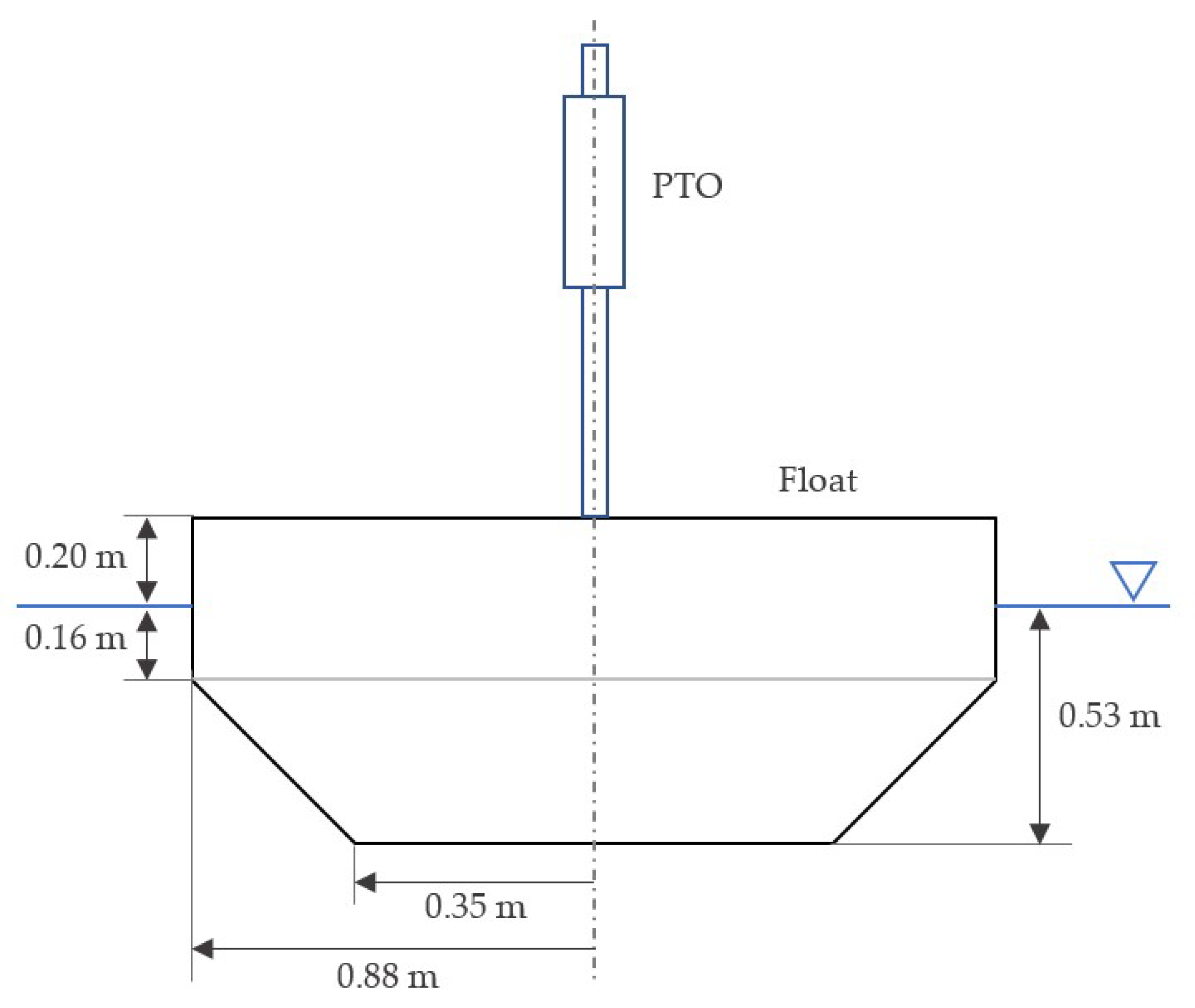
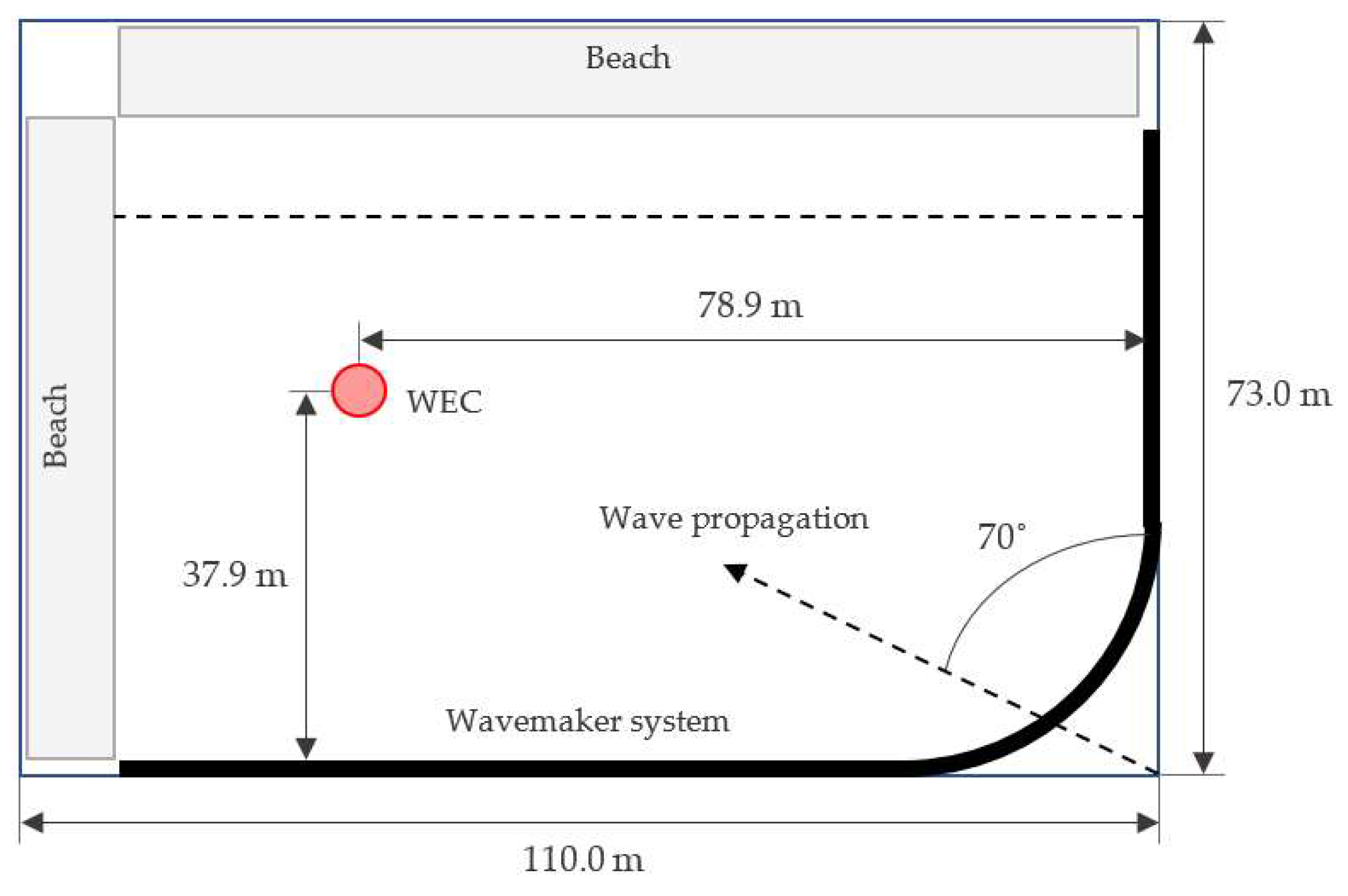
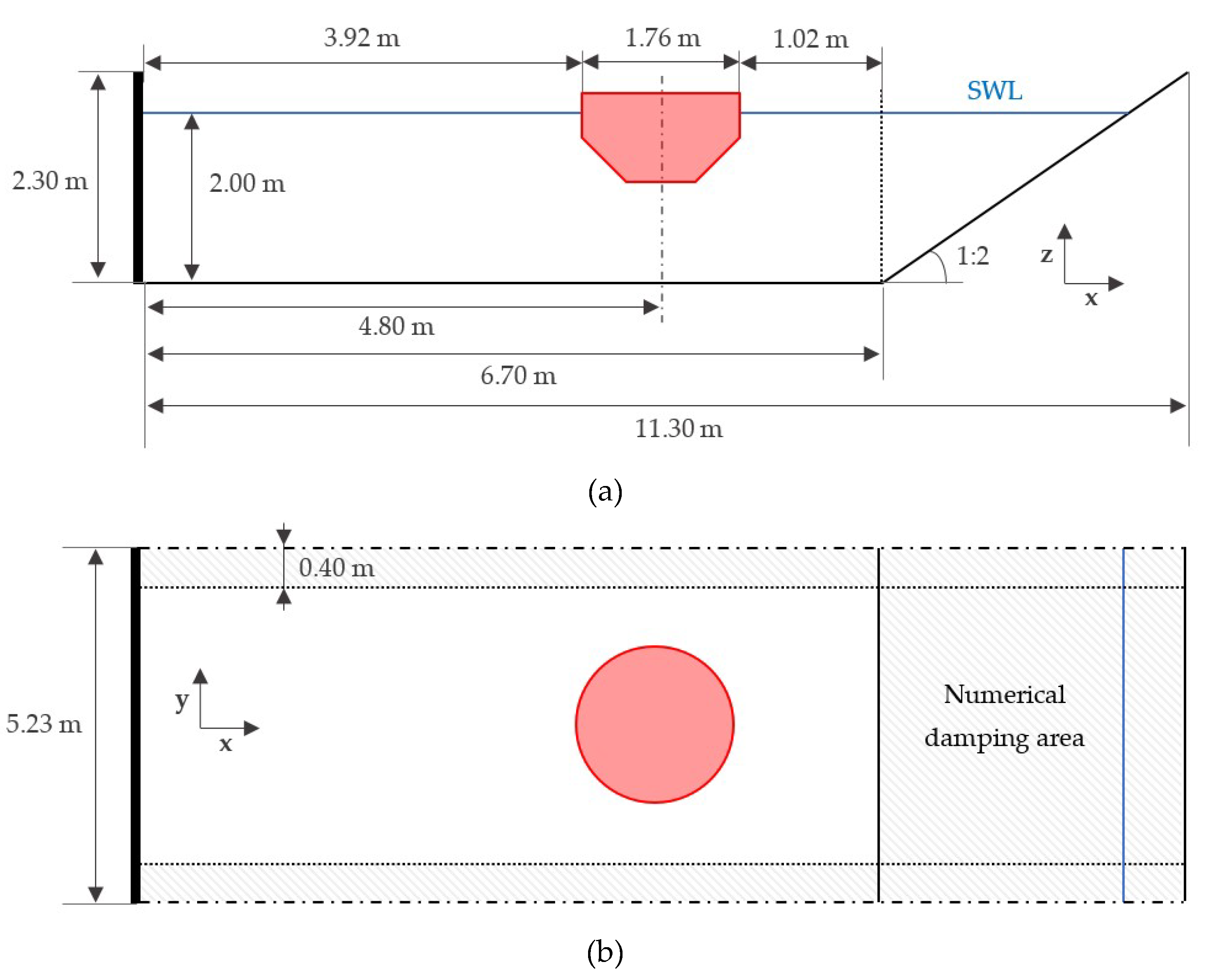
3. Experimental Campaign

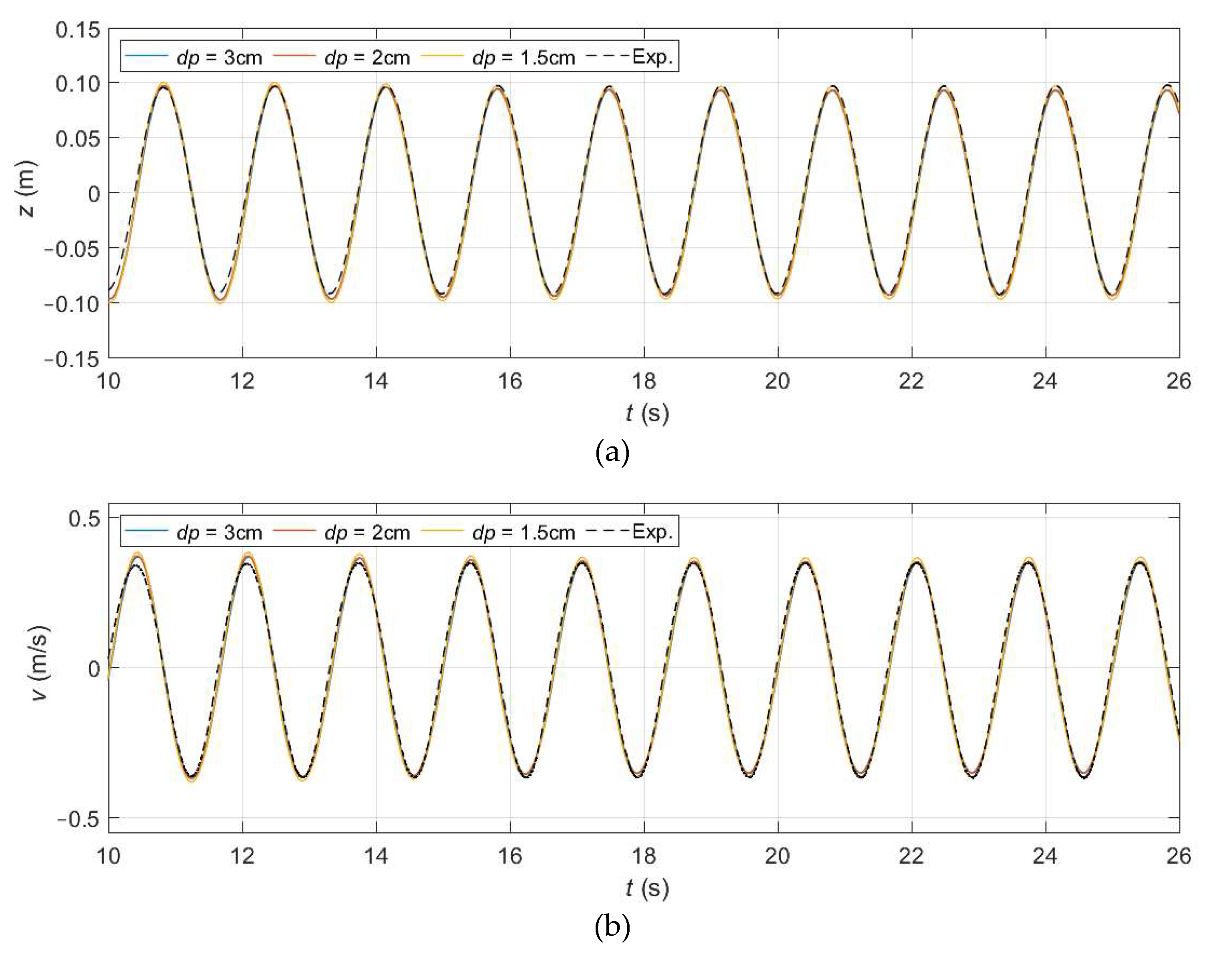
The WEC device studied here is a roughly 1/17th-scale model designed by Sandia National Laboratories [55]. It is schematically depicted in Figure 1 and its most relevant physical parameters are summarized in

Table 1. Model-scale wave energy converter (WEC) physical parameters.

Parameter	Symbol (Unit)	Value
Rigid-body mass (float and slider)	M (kg)	858
Displaced volume	V (m3)	0.858
Float radius	R (m)	0.88
Float draft	D (m)	0.53

. This device was designed to work in three degrees-of-freedom: heave, surge and pitch. However, for cases considered in this study, the surge and pitch motions are locked and the device is allowed to move in heave only. During the experiments, the effect of the PTO system is reproduced by means of an actuator located on top of the float, as shown in Figure 1. Therefore, the total rigid-body mass is the sum of the masses of the float and the actuator slider, as noted in Table 1. The vertical position of the float is measured by the sinusoidal encoder of the actuator, while the vertical force is measured by load cells. More information about the experimental data acquisition can be found in [55,56,57].

Physical tests were conducted in the Maneuvering and Sea Keeping (MASK) basin located in the Naval Surface Warfare Center, Carderock Division. As shown in Figure 2, the MASK basin is 110 m long, 73 m wide and 6.1 m deep, except for a 15.2 m wide trench parallel to the long side of the basin (dashed line), which has a depth of 10.7 m. Waves were sent diagonally across the basin. The MASK basin is spanned by a 115 m bridge (not shown in Figure 2 for the sake of simplicity), which can move, thanks to a rail system, to the center of the basin width as well as rotate up to 45° from the centerline. The MASK basin carriage, where the models and instrumentation are mounted, is suspended beneath the bridge, and is permitted to travel along the rails. The basin is equipped with a wavemaker system consisting of 216 paddles: 108 paddles along the long side of the basin, 60 paddles in a ninety-degree arc, and 48 paddles along the short edge of the basin. Two artificial beaches, with a 12° slope, are used to avoid wave reflections from the two edges opposite to the wavemakers. Note that the numerical tanks that will be used for the simulations in the next sections aim to reproduce the same wave–WEC interactions as in the wave basin (Figure 2). Several reductions in the tank dimensions were applied to reduce the computational runtime, however, due to the geometry of the float, it is necessary to keep all the simulations in 3D.

In this research, data from three different experimental campaigns were used: the MASK1, MASK2B and MASK3 campaigns. All of them were conducted by SANDIA National Laboratories between the years 2016 and 2019 and are publicly available at [55,56,57].

4. Radiation Test

Radiation tests consist of forcing the WEC in otherwise calm water with a known force in the vertical direction via its actuator. In the same fashion as the physical tests, the WEC’s motion is numerically restricted such that the float can only move in heave. The results shown in this section consider first a monochromatic force signal (F) and then a multisine force signal as inputs. The block diagram in Figure 3 shows that the radiation FRF (frequency-response-function) is the inverse of the intrinsic impedance, Z_i, while the output obtained from the radiation test is the heaving velocity, v, which can be calculated as

$$\mathit{v}=\frac{1}{Z_i}F.$$

(9)

A suitable numerical tank was designed to perform the radiation tests (the top view is shown in Figure 4). Since the goal of the numerical tank is to mimic open-sea conditions, it is necessary to avoid reflection from any of the boundaries. For this reason, the tank has a depth of 1.50 m and the lateral 7.20 m long boundaries form a square with the axisymmetric WEC at its center. Furthermore, periodic conditions [58] are applied to the lateral boundaries and numerical damping is applied to the lateral and bottom water particles, affecting those particles located less than 0.60 m away from the laterals and/or less than 0.20 m away from the bottom. The numerical damping system [59] employs a quadratic decay function to gradually reduce the velocity of fluid particles within the damping zone at each time step according to their location.

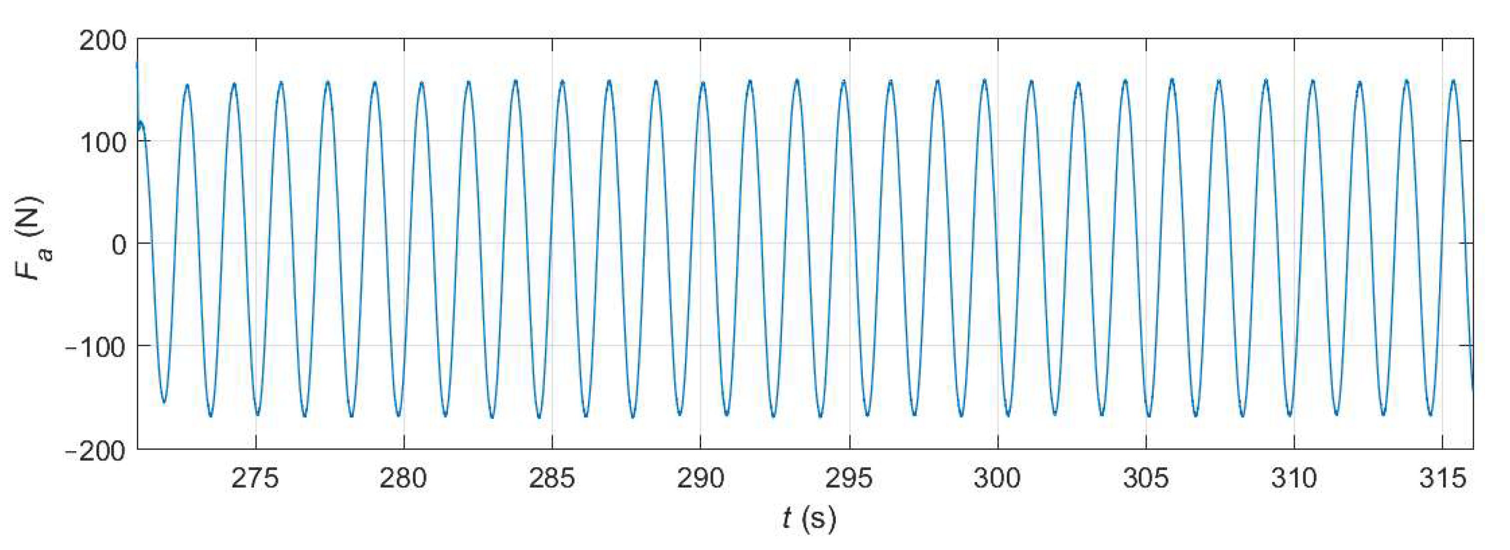
4.1. Monochromatic Force Signal

The monochromatic force input considered here is the one from Case130 of the MASK3 experimental campaign [57]: a sinusoidal signal with an amplitude of 800 N and a frequency of 0.60 Hz, which corresponds to a period of 1.67 s.

Using the same numerical tank described in Figure 4, different simulations for several resolutions are executed. In the SPH simulations, the resolution is defined by the initial interparticle distance, dp, which is employed to generate the particles that will initially discretize the numerical domain. In this case, three values of the initial interparticle distance are chosen: dp = 3.0, 2.0, 1.5 cm.

The WEC’s heave response, in terms of position (z) and velocity (v), for each resolution is shown in Figure 5 and compared with the corresponding experimental time series. It can be noted that the device reaches a steady state in which it oscillates harmonically with the frequency of the actuator force signal. Figure 5 also shows that the heave position and velocity time series satisfy the π/2 rad theoretical phase lag expected between them. Qualitatively, the matching between the numerical and experimental results observed in Figure 5 is satisfactory, both in amplitude and phase, for all resolutions.

To quantify the accuracy of the results, the non-dimensional error estimator named index of agreement, d₁, is employed. According to [60], it can be defined in a general way as:

$$d_1=1-\frac{{{\displaystyle \sum }}_{n=1}^N\left|C_n-E_n\right|}{{{\displaystyle \sum }}_{n=1}^N\left(\left|C_n-\overline{E}\right|+\left|E_n-\overline{E}\right|\right)},$$

(10)

N being the total number of records of the variable, C and E its numerical and experimental values, respectively, and the overbar indicates average. Equation (10) shows that d₁ is bounded between zero and one, where one represents perfect agreement between the two signals.

Table 2. Number of particles, number of total time steps, runtime and index of agreement for three values of dp.

dp (cm)	Particles	Time Steps	Runtime (h)	d1
				z	v
1.5	24.1 × 106	3.4 × 105	132.6	0.97	0.96
2.0	10.3 × 106	2.6 × 105	53.6	0.97	0.96
3.0	3.1 × 106	1.7 × 105	10.6	0.96	0.96

shows the index of agreement, total number of particles and runtime for each simulation. The computational times shown in Table 2 correspond to 26 s of physical time simulated in a GeForce RTX 2080 GPU card. Note that the lower the dp, the more particles involved in the simulation and the longer the execution time. The values of d₁ confirm that results are highly accurate for the three values of dp and only a slight improvement is achieved when the two finest resolutions are used.

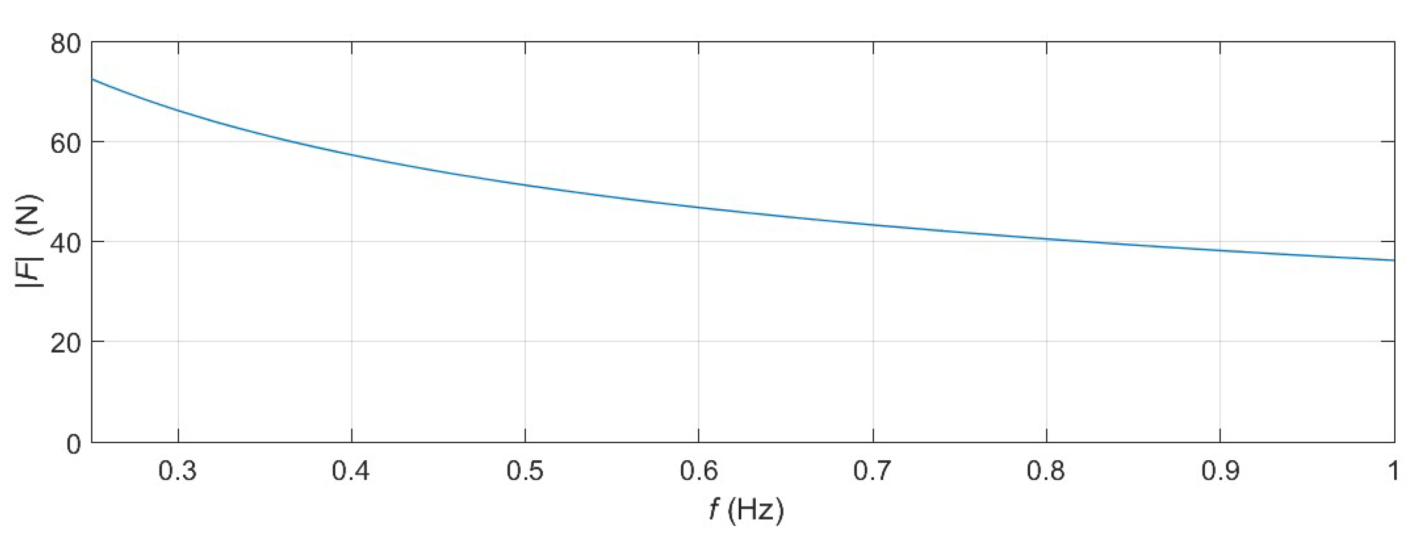
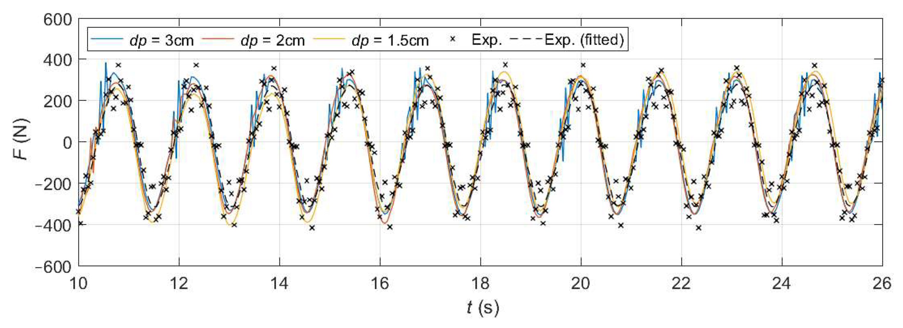
4.2. Polychromatic Force Signal

In this section, a multisine force signal is applied to the WEC in order to obtain the intrinsic impedance of the system and its resonant frequency. This allows the performance an interesting comparison in the frequency domain between results from DualSPHysics, physical experiments and potential-flow code WAMIT. Figure 6 shows that the input force, which covers a range of frequencies from 0.25 to 1.00 Hz, is a pink multisine signal, since its amplitude (and therefore, its power spectral density) decreases with frequency. To set the resolution and length of the input force signal, a compromise between accuracy and computational cost must be achieved. Table 2 shows that the accuracy is slightly improved at a reasonable computational cost when using dp = 2.0 cm, and Figure 7a shows that the magnitude of the force applied is, especially at certain instants, significantly lower than in the monochromatic case. Therefore, dp = 2.0 cm is used here. To keep the computational times lower than a week (using a GeForce RTX 2080 GPU card), a single period of 100 s of the multisine signal is employed.

Figure 7b depicts the heave velocity response, v, obtained when the force signal, F, shown in Figure 7a, is applied to the device. Since the input signal is periodic (even though only one period is considered), the force and velocity can be described by their complex quantities in the frequency-domain, denoted as $\widehat{F}$ and $\widehat{\mathit{v}}$, respectively. In this way, the block diagram in Figure 3 and Equation (9) show that the intrinsic impedance can be obtained as:

$$Z_i=\frac{\widehat{F}}{\widehat{\mathit{v}}},$$

(11)

where $\widehat{F}$ and $\widehat{\mathit{v}}$ are calculated from their time series (Figure 7) using the discrete Fourier transform via the Fast Fourier Transform (FFT).

The same procedure is used to obtain the intrinsic impedance from the experimental force input signal and heave velocity output [61]. More specifically, data from Case063 of the MASK2B experimental campaign [56] are considered here, where a single period of a pink multisine signal is also used but, in this case, with a total period of 300 s (instead of the 100 s period used in the SPH simulation). This difference between the numerical and experimental periods is important because the lower the period, the fewer frequency components considered, i.e., lower frequency resolution. This is because the frequency sampling is inversely proportional to the period thus, in this case, the frequency sampling is 1/100 Hz for numerical results and 1/300 Hz for experimental results.

The intrinsic impedance is a frequency dependent complex-valued variable that accounts for the effects of inertia, radiation, viscosity and hydrostatic stiffness. According to [62], the intrinsic impedance, Z_i(ω), can be modelled as:

$$Z_i\left(\omega \right)=b_f+b_r\left(\omega \right)+i\left(\omega \left(M+m_a\left(\omega \right)\right)-\frac{k_{hs}}{\omega }\right),$$

(12)

where the viscous force has been assumed to be linear with velocity via a friction coefficient, b_f, the radiation force is defined by the radiation damping, b_r, and the added mass, m_a, the hydrostatic force depends on the hydrostatic coefficient, k_hs, and the inertia force simply depends on the mass of the device, M. It is important to note that Equations (11) and (12) allow attainment of the resonance frequency of the device, i.e., the frequency at which resonance is achieved. As stated in [62], resonance occurs when the heave velocity is in phase with the excitation force. Thus, the resonance frequency is the one that guarantees that Im(Z_i) = 0 Ns/m (which directly implies ∠Z_i = 0 rad).

Figure 8 depicts the magnitude (top left), phase (bottom left), real part (top right) and imaginary part (bottom right) of the intrinsic impedance in the frequency domain. The results of the DualSPHysics simulation (in blue) are compared with the experimental ones (in orange) [61] and with the ones calculated using the potential-flow method WAMIT (in black). Both signals, the experimental and SPH one, have some noise; this noise being more relevant in the latter due to the lower frequency resolution employed, as previously explained. To avoid this undesirable but inevitable effect, a second order Savitzky-Golay filter is used to smooth the SPH and experimental results (dashed lines in Figure 8). Leaving aside the plot of Re(Z_i), Figure 8 demonstrates a high level of agreement between the SPH, experimental and WAMIT results. The resonance frequency, obtained as the frequency at which the imaginary part (or, equivalently, the phase) of the intrinsic impedance crosses the x-axis, is around 0.65 Hz for all cases. Regarding the plot of the real part of Z_i shown in Figure 8, the difference between the experimental and WAMIT curves is roughly constant with frequency, revealing an offset caused by the fact that WAMIT is neglecting the viscous effects, which have a significant impact on Re(Z_i), as shown in Equation (12). This mismatch was investigated in depth in [61]. The real part of the intrinsic impedance obtained with SPH nicely matches the experimental data at high frequencies; however, when low frequencies are considered, Re(Z_i) is highly underestimated. This means that when the frequency is high enough, the SPH simulation is able to reproduce the physics of the problem correctly, but when the frequency is low, there is a phenomenon, most likely related with viscosity, that is not being adequately captured.

5. Static and Dynamic Response Test

In this section, the effect of incoming waves on the WEC is considered. First, a static excitation test is conducted by keeping the device fixed and calculating the forces exerted by regular waves of height H = 0.09 m and period T = 1.54 s (which corresponds to a wavelength L = 3.70 m in deep-water conditions). Then, during the dynamic response test the device is allowed to oscillate, and its heave response is calculated as a result of the incoming waves and the actuator force. The regular waves have, in this case, a wave height of H = 0.11 m and period of T = 1.58 s (corresponding, in deep water, to a wavelength of L = 3.90 m).

The numerical domain employed in the simulations is common for the two aforementioned cases since the wave conditions are very similar. A detailed diagram of the top and lateral views of the numerical domain is shown in Figure 9. Although the numerical tank is very different from the experimental basin to reduce the computational runtime, it has been carefully designed such that the wave conditions acting on the device are the same. The reduction in the water depth from 6.10 m to 2.00 m is such that the deep-water condition present in the experimental campaign is conserved and, therefore, the wavelength remains constant. The correct wave propagation is guaranteed by placing the device one wavelength away from the wavemaker (considering the case with longer waves). The wavemaker consists of 17 independent pistons, each one equipped with an active wave absorption system [59] that absorbs the waves radiated by the device, guaranteeing an adequate wave generation throughout the entire simulation. To avoid lateral reflection, the width of the numerical domain is set to 5.23 m (roughly three times the buoy diameter). In addition, periodic boundary conditions are also applied in the lateral limits, and the numerical damping mechanism described in Section 4 is used in the 0.40-m wide zones closer to the lateral boundaries (to damp the transversal velocities). Finally, a 1:2 steep beach together with numerical damping (to damp the longitudinal velocities) prevents any possible reflection downstream of the device. The overall absorption capabilities of the beach and numerical damping used together here are above 96% for both wave conditions, which means that over 96% of the incident wave energy is being dissipated.

5.1. Static Response Test

The physical test Case004 from the MASK1 campaign [55] is replicated here numerically using the DualSPHysics code. It consists of obtaining the forces exerted by regular waves of height H = 0.09 m and period T = 1.54 s (which corresponds to L = 3.70 m) on a fixed WEC. Denoting the free-surface elevation with η, its block diagram is shown in Figure 10.

Figure 11 shows the experimental and numerical time series of the vertical force acting on the buoy for three different resolutions, namely dp = 3.0, 2.0 and 1.5 cm. In this figure, the exact instantaneous values of the experimental force are depicted with black crosses while the corresponding fitted curve, generated using a fourth order Savitzky-Golay function, is represented by a black dashed line. As expected, the obtained responses, both numerical and experimentally, are sinusoidal and their periods are equal to the wave period. The figure shows, qualitatively, that the results obtained with any of the resolutions employed provide a good matching, in terms of amplitude and phase, with the experimental curve. Note, nevertheless, that the force output obtained with dp = 3.0 cm presents an important amount of noise during its peaks, while finer resolutions do not. The index of agreement, d₁, defined in Equation (10) is used here as a quantitive measure of the total error in each case. Its values, shown in

Table 3. Number of particles, number of total time steps, runtime and index of agreement for three values of dp.

dp (cm)	Particles	Time Steps	Runtime (h)	d1
1.5	28.1 × 106	3.7 × 105	157.8	0.90
2.0	12.1 × 106	2.8 × 105	63.5	0.89
3.0	3.7 × 106	1.9 × 105	10.4	0.89

, certify the good matching observed in Figure 11, as well as the fact that the accuracy slightly improves when decreasing dp. Table 3 also includes the runtimes of the execution of 26 s of physical time using the same GPU card indicated before.

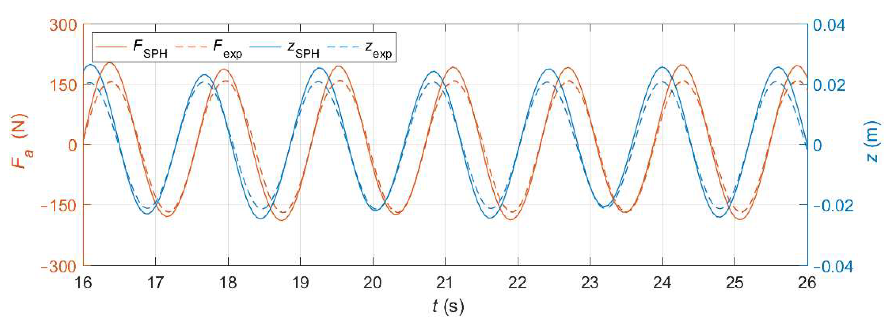
5.2. Dynamic Response Test

During the dynamic response test, the WEC moves in heave under the action of waves and the actuator force, F_a. This actuator force may be either predefined externally (open-loop system) or defined during the test by means of the feedback provided by the PTO (closed-loop system). Both possibilities, depicted in Figure 12 via block diagrams, are considered in this section based on Case149 of the MASK3 experimental campaign [57]. During the experiment, the actuator force applied to the WEC is the reaction of the PTO force, i.e., F_a = − F_PTO; F_PTO being modelled as a proportional–integral (PI) controller that depends on the device’s heave position, z, and velocity, v [63]:

$$F_{PTO}=k_{PTO}z+b_{PTO}v,$$

(13)

where k_PTO and b_PTO are, respectively, the stiffness and damping coefficient of the PTO system or, equivalently, the integral and proportional gains of the PI controller.

To search the space of controller gains for the optimal tuning around a predicted value, the proportional and integral gains vary every 45 s during the physical experiment. In this section, however, a time window where the gains remain constant is selected from the physical experiment [57]. In particular, t ∈ (271,316) is considered, where the actuator force (shown in Figure 13) is defined by k_PTO = 3527 N/m and b_PTO = −1754 Ns/m. The wave conditions remain constant throughout the entire experiment: regular waves of height H = 0.11 m and period T = 1.58 s, which qualifies as a deep-water wave with a wavelength of L = 3.90 m. Figure 13 shows that, as expected, the frequency of the actuator force is coincident with the wave frequency and that, after the transient observed during the first period, its amplitude is approximately constant around 160 N. This initial transient is avoided in the simulations by considering the time series from t = 273 s.

The numerical tank shown in Figure 9 is employed in all the simulations in this section. From the information available in Table 2 and Table 3, it is concluded that dp = 2 cm provides a good compromise between accuracy and computational cost, while avoiding any possible noise in the results.

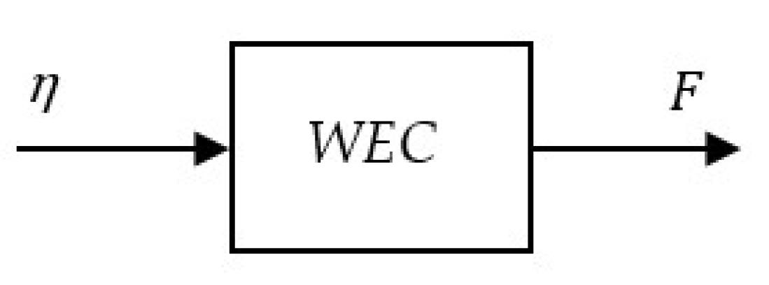
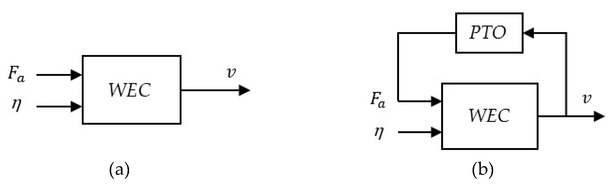
5.2.1. Open-Loop System

The time series of the experimental actuator force (Figure 13) is applied here to the numerical device as a predefined input signal in DualSPHysics. The WEC’s heave response is the result of the interaction between the externally-imposed actuator force and the action of regular waves. Therefore, the phase between the wave elevation and the actuator force has a very important effect on the results. Even though it is not possible to know with certainty the wave elevation at the WEC location, the heave position z is available and its phase with respect to F_a can be effectively used instead. Three different phases are simulated simply by delaying the time at which the external actuator force is applied in each simulation (cases A, B and C). The actuator force and heave position time series for the three numerical cases are shown, along with the experimental ones, in Figure 14. Regarding the numerical results, the actuator force signal is shifting in phase while the heave position is not, causing a phase difference between them of about π rad in case A, 3π/4 rad in case B, and π/2 rad in case C. The experimental phase between F_a and z, observed in the bottom plot of Figure 14, is very similar to the one obtained with case C, i.e., approximately π/2 rad.

Figure 15 compares the heave position and velocity time series of each numerical case with the experimental results. The three cases overestimate the amplitudes of z and v but, as the phase lag between F_a and z approaches the experimental one (Figure 14), so do the amplitudes of the heave position and velocity. However, the phase difference is not known before running the simulation, thus it becomes a trial-and-error process. This approach, besides being inefficient, is also unrealistic because the actuator force is very rarely given by a predefined signal, but rather by its PTO force.

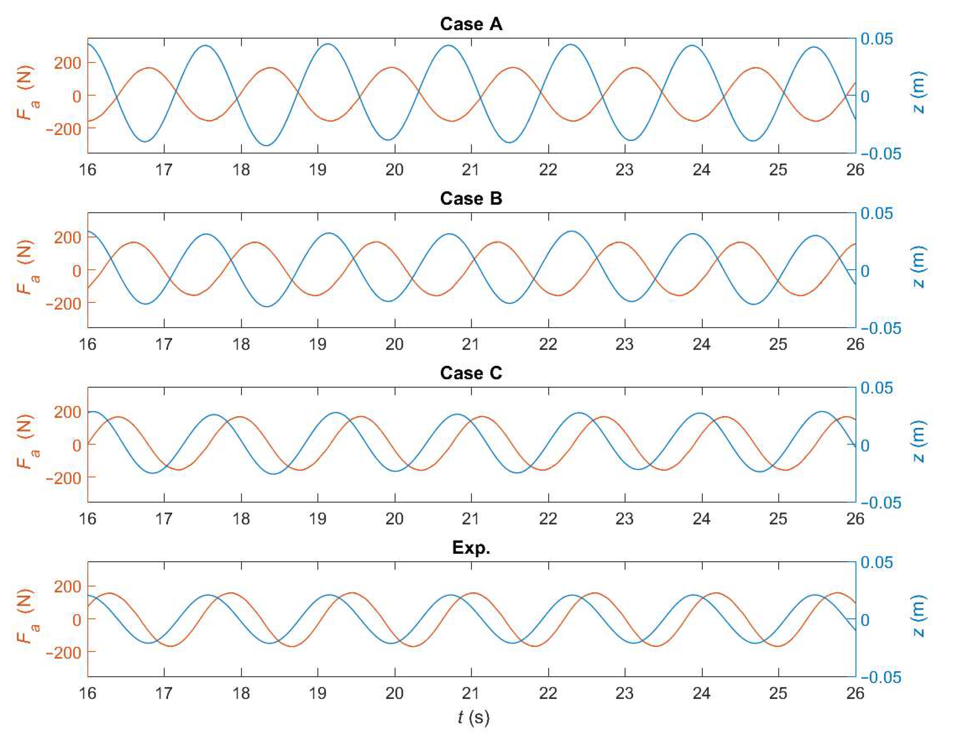
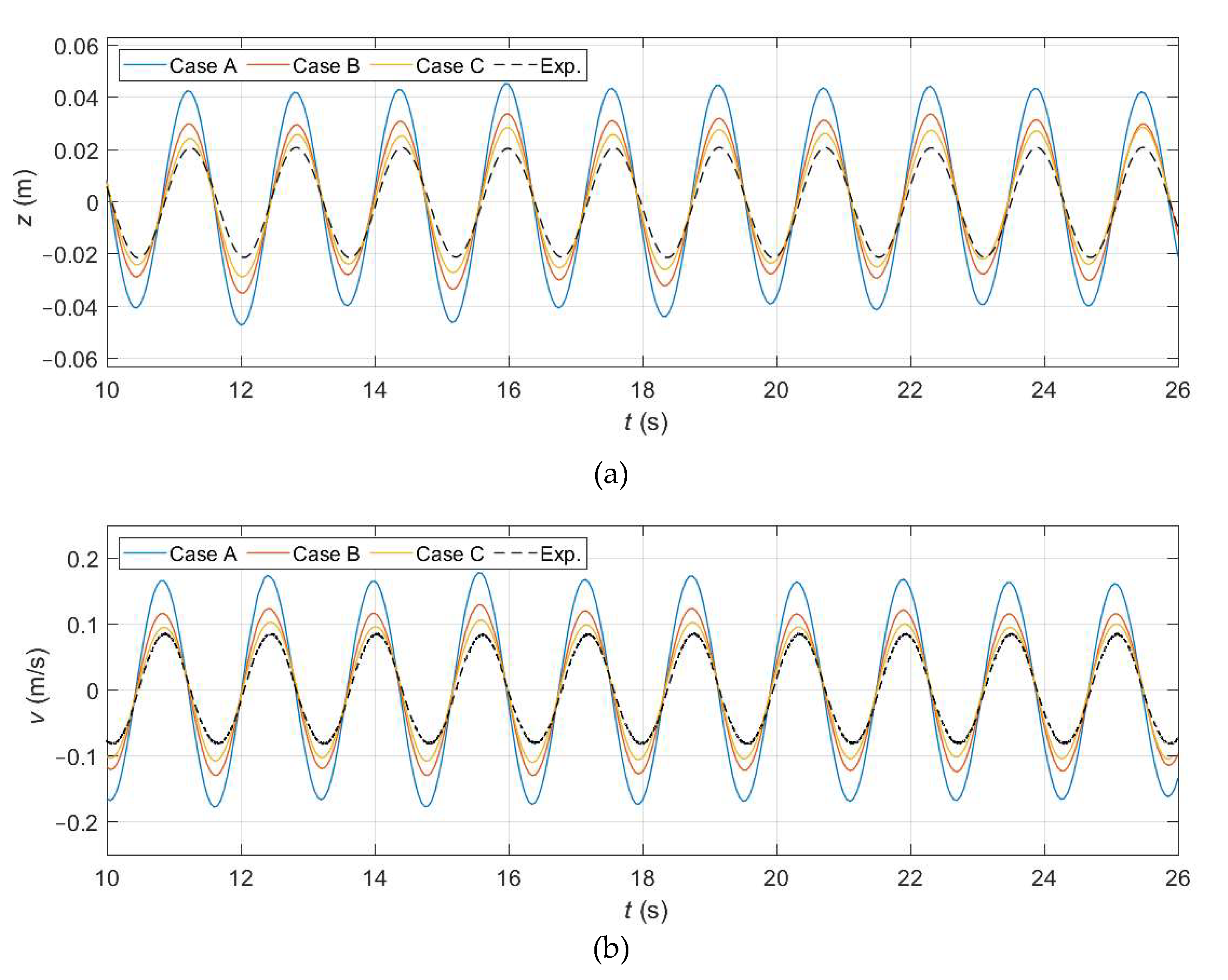
5.2.2. Closed-Loop System

The actuator force is applied to the WEC in the physical experiment [57] by means of a closed-loop system as the reaction of the PTO force. The PTO force depends on the device’s heave response according to the coefficients k_PTO and b_PTO, as described in Equation (13). Project Chrono allows numerical implementation of this feedback loop simply by setting k_PTO = 3527 N/m and b_PTO = −1754 Ns/m. Therefore, thanks to the coupling of DualSPHysics with Project Chrono it is possible to simulate the dynamic response test with its corresponding closed-loop system using the numerical tank defined in Figure 9 and the wave conditions previously described (H = 0.11 m and T = 1.58 s).

Figure 16 shows the numerical (solid lines) and experimental (dashed lines) time series of the actuator force and heave position. The numerical phase difference between F_a and z now matches the experimental one. This is automatically accomplished because the actuator force is being calculated at each time step as a function of the instantaneous heave position and velocity, instead of being pre-imposed externally.

Figure 17 shows the heave position and velocity obtained numerically and experimentally. The matching in terms of phase is nearly perfect, while in terms of amplitude it is slightly overestimated. If the index of agreement (Equation (10)) is used to quantify the error, a value of d₁ = 0.92 is obtained for both z and v when using a closed-loop system, which is significantly higher than the one obtained with the most accurate case when using an open-loop system (d₁ = 0.74). By comparing results in Figure 17 with the ones in Figure 15, it can be also seen that the amplitude overestimation obtained now with a closed-loop system is lower than in any of the three cases with an open-loop system. Note as well that the amplitude of the heave movement is of approximately 0.02 m, which is the value of the dp used, meaning that small motions can be correctly simulated even with relatively coarse resolutions. Therefore, this numerical simulation satisfactorily reproduces the response of the WEC equipped with a proportional–integral controller.

6. Conclusions

This work aims to prove the capability of the DualSPHysics code coupled with the multiphysics Project Chrono library to reproduce the behavior of a point-absorber under different conditions, including the closed-loop controller defined by the PTO system. By comparing numerical results with physical tests conducted by Sandia National Laboratories, DualSPHysics has proved to be a valuable numerical tool to conduct experiments that are fundamental during the design stage of point absorbers. In this work, results were only compared in terms of the forces acting on the WEC and its motions; however, DualSPHysics also has the ability to easily calculate other parameters (such as pressure, particles trajectories or the vorticity field) that can be useful when modelling and optimizing WECs in future works.

The radiation models built from the WAMIT and DualSPHysics simulations were compared with the experimental model by plotting the intrinsic impedance calculated in each case in the frequency domain. It was found that the SPH results match the experimental ones except for the real part of Z_i at low frequencies, that is significantly underestimated. On the other hand, WAMIT also provides good results except for Re(Z_i), which is underestimated at all frequencies. This offset, which is roughly constant with frequency, is due to the fact that the potential-flow solver neglects viscosity. Thus, the most efficient way to numerically obtain the radiation model is to use WAMIT (or another potential-flow solver) but adding a correction that takes into account the viscous effects. The proven ability of the SPH method to reproduce the viscous effects at high frequencies allows for an estimation of the viscous correction needed for the potential-flow solver. Therefore, a fast and reliable procedure for system identification can be set up by combining the results obtained with a CFD simulation and a potential solver.

It has been shown that the heave response of the device forced via its actuator in calmed water can be accurately obtained even using coarse resolutions with DualSPHysics. The forces exerted by regular waves on the fixed WEC have also been correctly calculated. Finally, during the dynamic response test (when both regular waves and the actuator force are applied simultaneously), it has been proven that the closed-loop system needs to be considered in order to reproduce the nature of the physical experiments. Thanks to the coupling of DualSPHysics with Project Chrono, it is possible to model the PTO force that defines the feedback loop. In this way, the experimental phase between the two inputs is automatically satisfied and the numerical heave response matches satisfactorily the experimental one.

References

1. Drew, B.; Plummer, A.; Sahinkaya, M. A Review of Wave Energy Converter Technology. Proc. Inst. Mech. Eng. Part J. Power Energy 2009, 223, 887–902. [Google Scholar] [CrossRef] [Green Version]
2. Babarit, A.; Hals, J.; Muliawan, M.J.; Kurniawan, A.; Moan, T.; Krokstad, J. Numerical Benchmarking Study of a Selection of Wave Energy Converters. Renew. Energy 2012, 41, 44–63. [Google Scholar] [CrossRef]
3. Magagna, D.; Monfardini, R.; Uihlein, A. JRC Ocean Energy Status Report 2016 Edition; Publications Office of the European Union: Luxembourg, 2016. [Google Scholar]
4. Hals, J.; Falnes, J.; Moan, T. A Comparison of Selected Strategies for Adaptive Control of Wave Energy Converters. J. Offshore Mech. Arct. Eng. 2011, 133, 031101. [Google Scholar] [CrossRef]
5. Coe, R.G.; Bacelli, G.; Wilson, D.G.; Abdelkhalik, O.; Korde, U.A.; Robinett III, R.D. A Comparison of Control Strategies for Wave Energy Converters. Int. J. Mar. Energy 2017, 20, 45–63. [Google Scholar] [CrossRef]
6. Bosma, B.; Lewis, T.; Brekken, T.; von Jouanne, A. Wave Tank Testing and Model Validation of an Autonomous Wave Energy Converter. Energies 2015, 8, 8857–8872. [Google Scholar] [CrossRef]
7. Kracht, P.; Perez-Becker, S.; Richard, J.-B.; Fischer, B. Performance Improvement of a Point Absorber Wave Energy Converter by Application of an Observer-Based Control: Results from Wave Tank Testing. IEEE Trans. Ind. Appl. 2015, 51, 3426–3434. [Google Scholar] [CrossRef]
8. Todalshaug, J.H.; Ásgeirsson, G.S.; Hjálmarsson, E.; Maillet, J.; Möller, P.; Pires, P.; Guérinel, M.; Lopes, M. Tank Testing of an Inherently Phase-Controlled Wave Energy Converter. Int. J. Mar. Energy 2016, 15, 68–84. [Google Scholar] [CrossRef]
9. Martin, D.; Li, X.; Chen, C.-A.; Thiagarajan, K.; Ngo, K.; Parker, R.; Zuo, L. Numerical Analysis and Wave Tank Validation on the Optimal Design of a Two-Body Wave Energy Converter. Renew. Energy 2020, 145, 632–641. [Google Scholar] [CrossRef]
10. Folley, M.; Babarit, A.; Child, B.; Forehand, D.; O’Boyle, L.; Silverthorne, K.; Spinneken, J.; Stratigaki, V.; Troch, P. A Review of Numerical Modelling of Wave Energy Converter Arrays. In Volume 7: Ocean Space Utilization; Ocean Renewable Energy; American Society of Mechanical Engineers: Rio de Janeiro, Brazil, 2012; pp. 535–545. [Google Scholar]
11. Penalba, M.; Ringwood, J. A Review of Wave-to-Wire Models for Wave Energy Converters. Energies 2016, 9, 506. [Google Scholar] [CrossRef] [Green Version]
12. Penalba, M.; Giorgi, G.; Ringwood, J.V. Mathematical Modelling of Wave Energy Converters: A Review of Nonlinear Approaches. Renew. Sustain. Energy Rev. 2017, 78, 1188–1207. [Google Scholar] [CrossRef] [Green Version]
13. Zabala, I.; Henriques, J.C.C.; Blanco, J.M.; Gomez, A.; Gato, L.M.C.; Bidaguren, I.; Falcão, A.F.O.; Amezaga, A.; Gomes, R.P.F. Wave-Induced Real-Fluid Effects in Marine Energy Converters: Review and Application to OWC Devices. Renew. Sustain. Energy Rev. 2019, 111, 535–549. [Google Scholar] [CrossRef]
14. Davidson, J.; Costello, R. Efficient Nonlinear Hydrodynamic Models for Wave Energy Converter Design—A Scoping Study. J. Mar. Sci. Eng. 2020, 8, 35. [Google Scholar] [CrossRef] [Green Version]
15. Li, Y.; Yu, Y.-H. A Synthesis of Numerical Methods for Modeling Wave Energy Converter-Point Absorbers. Renew. Sustain. Energy Rev. 2012, 16, 4352–4364. [Google Scholar] [CrossRef]
16. Beatty, S.J.; Hall, M.; Buckham, B.J.; Wild, P.; Bocking, B. Experimental and Numerical Comparisons of Self-Reacting Point Absorber Wave Energy Converters in Regular Waves. Ocean Eng. 2015, 104, 370–386. [Google Scholar] [CrossRef]
17. de Andrés, A.D.; Guanche, R.; Armesto, J.A.; del Jesus, F.; Vidal, C.; Losada, I.J. Time Domain Model for a Two-Body Heave Converter: Model and Applications. Ocean Eng. 2013, 72, 116–123. [Google Scholar] [CrossRef]
18. Rahmati, M.T.; Aggidis, G.A. Numerical and Experimental Analysis of the Power Output of a Point Absorber Wave Energy Converter in Irregular Waves. Ocean Eng. 2016, 111, 483–492. [Google Scholar] [CrossRef] [Green Version]
19. Cummins, W.E. The Impulse Response Function and Ship Motions; David Taylor Model Basin Reports; University of Hamburg, Department of the Navy, Hydromechanics Laboratories: Hamburg, Germany, 1962. [Google Scholar]
20. Lee, C.H. WAMIT Theory Manual; Massachusetts Institute of Technology, Department of Ocean Engineering: Cambridge, MA, USA, 1995. [Google Scholar]
21. Babarit, A.; Delhommeau, G. Theoretical and Numerical Aspects of the Open Source BEM Solver NEMOH. In Proceedings of the 11th European Wave and Tidal Energy Conference, Nantes, France, 1 September 2015. [Google Scholar]
22. Yu, Y.-H.; Li, Y. Reynolds-Averaged Navier–Stokes Simulation of the Heave Performance of a Two-Body Floating-Point Absorber Wave Energy System. Comput. Fluids 2013, 73, 104–114. [Google Scholar] [CrossRef]
23. Sjökvist, L.; Wu, J.; Ransley, E.; Engström, J.; Eriksson, M.; Göteman, M. Numerical Models for the Motion and Forces of Point-Absorbing Wave Energy Converters in Extreme Waves. Ocean Eng. 2017, 145, 1–14. [Google Scholar] [CrossRef] [Green Version]
24. Jin, S.; Patton, R.J.; Guo, B. Viscosity Effect on a Point Absorber Wave Energy Converter Hydrodynamics Validated by Simulation and Experiment. Renew. Energy 2018, 129, 500–512. [Google Scholar] [CrossRef]
25. Reabroy, R.; Zheng, X.; Zhang, L.; Zang, J.; Yuan, Z.; Liu, M.; Sun, K.; Tiaple, Y. Hydrodynamic Response and Power Efficiency Analysis of Heaving Wave Energy Converter Integrated with Breakwater. Energy Convers. Manag. 2019, 195, 1174–1186. [Google Scholar] [CrossRef]
26. Coe, R.G.; Rosenberg, B.J.; Quon, E.W.; Chartrand, C.C.; Yu, Y.-H.; van Rij, J.; Mundon, T.R. CFD Design-Load Analysis of a Two-Body Wave Energy Converter. J. Ocean Eng. Mar. Energy 2019, 5, 99–117. [Google Scholar] [CrossRef]
27. Gomez-Gesteira, M.; Rogers, B.D.; Dalrymple, R.A.; Crespo, A.J.C. State-of-the-Art of Classical SPH for Free-Surface Flows. J. Hydraul. Res. 2010, 48, 6–27. [Google Scholar] [CrossRef]
28. Gotoh, H.; Khayyer, A. On the State-of-the-Art of Particle Methods for Coastal and Ocean Engineering. Coast. Eng. J. 2018, 60, 79–103. [Google Scholar] [CrossRef]
29. Rafiee, A.; Elsaesser, B.; Dias, F. Numerical Simulation of Wave Interaction with an Oscillating Wave Surge Converter. In Volume 5: Ocean Engineering; American Society of Mechanical Engineers: Nantes, France, 2013; p. V005T06A013. [Google Scholar]
30. Edge, B.L.; Gamiel, K.; Dalrymple, R.A.; Hérault, A.; Bilotta, G. Application of Gpusph to Design of Wave Energy. In Proceedings of the 9th SPHERIC International Workshop, Paris, France, 2–5 June 2014. [Google Scholar]
31. Westphalen, J.; Greaves, D.M.; Raby, A.; Hu, Z.Z.; Causon, D.M.; Mingham, C.G.; Omidvar, P.; Stansby, P.K.; Rogers, B.D. Investigation of Wave-Structure Interaction Using State of the Art CFD Techniques. Open J. Fluid Dyn. 2014, 04, 18–43. [Google Scholar] [CrossRef] [Green Version]
32. Omidvar, P.; Stansby, P.K.; Rogers, B.D. SPH for 3D Floating Bodies Using Variable Mass Particle Distribution: SPH FOR 3D FLOATING BODIES USING VARIABLE MASS PARTICLE DISTRIBUTION. Int. J. Numer. Methods Fluids 2013, 72, 427–452. [Google Scholar] [CrossRef]
33. Yeylaghi, S.; Moa, B.; Beatty, S.; Buckham, B.; Oshkai, P.; Crawford, C. SPH Modeling of Hydrodynamic Loads on a Point Absorber Wave Energy Converter Hull. In Proceedings of the 11th European Wave and Tidal Energy Conference, Nantes, France, 1 September 2015. [Google Scholar]
34. Crespo, A.J.C.; Domínguez, J.M.; Rogers, B.D.; Gómez-Gesteira, M.; Longshaw, S.; Canelas, R.; Vacondio, R.; Barreiro, A.; García-Feal, O. DualSPHysics: Open-Source Parallel CFD Solver Based on Smoothed Particle Hydrodynamics (SPH). Comput. Phys. Commun. 2015, 187, 204–216. [Google Scholar] [CrossRef]
35. Tasora, A.; Serban, R.; Mazhar, H.; Pazouki, A.; Melanz, D.; Fleischmann, J.; Taylor, M.; Sugiyama, H.; Negrut, D. Chrono: An Open Source Multi-Physics Dynamics Engine. In High Performance Computing in Science and Engineering; Kozubek, T., Blaheta, R., Šístek, J., Rozložník, M., Čermák, M., Eds.; Springer International Publishing: Cham, Switzerland, 2016; Volume 9611, pp. 19–49. [Google Scholar]
36. Crespo, A.J.C.; Hall, M.; Domínguez, J.M.; Altomare, C.; Wu, M.; Verbrugghe, T.; Stratigaki, V.; Troch, P.; Gómez-Gesteira, M. Floating Moored Oscillating Water Column With Meshless SPH Method. In Volume 11B: Honoring Symposium for Professor Carlos Guedes Soares on Marine Technology and Ocean Engineering; American Society of Mechanical Engineers: Madrid, Spain, 2018; p. V11BT12A053. [Google Scholar]
37. Brito, M.; Canelas, R.B.; García-Feal, O.; Domínguez, J.M.; Crespo, A.J.C.; Ferreira, R.M.L.; Neves, M.G.; Teixeira, L. A Numerical Tool for Modelling Oscillating Wave Surge Converter with Nonlinear Mechanical Constraints. Renew. Energy 2020, 146, 2024–2043. [Google Scholar] [CrossRef]
38. Ropero-Giralda, P.; Crespo, A.J.C.; Tagliafierro, B.; Altomare, C.; Domínguez, J.M.; Gómez-Gesteira, M.; Viccione, G. Efficiency and Survivability Analysis of a Point-Absorber Wave Energy Converter Using DualSPHysics. Renew. Energy 2020, 162, 1763–1776. [Google Scholar] [CrossRef]
39. Monaghan, J.J. Smoothed Particle Hydrodynamics. Annu. Rev. Astron. Astrophys. 1992, 30, 543–574. [Google Scholar] [CrossRef]
40. Wendland, H. Piecewise Polynomial, Positive Definite and Compactly Supported Radial Functions of Minimal Degree. Adv. Comput. Math. 1995, 4, 389–396. [Google Scholar] [CrossRef]
41. Fourtakas, G.; Domínguez, J.M.; Vacondio, R.; Rogers, B.D. Local Uniform Stencil (LUST) boundary condition for arbitrary 3-D boundaries in parallel smoothed particle hydrodynamics (SPH) models. Computers & Fluids 2019, 190, 346–361. [Google Scholar] [CrossRef]
42. Ma, Q. Advances in Numerical Simulation of Nonlinear Water Waves. World Sci. 2010, 11. [Google Scholar] [CrossRef]
43. Vacondio, R.; Altomare, C.; De Leffe, M.; Hu, X.; Le Touzé, D.; Lind, S.; Marongiu, J.-C.; Marrone, S.; Rogers, B.D.; Souto-Iglesias, A. Grand Challenges for Smoothed Particle Hydrodynamics Numerical Schemes. Comput. Part. Mech. 2020. [Google Scholar] [CrossRef]
44. Crespo, A.J.C.; Gómez-Gesteira, M.; Dalrymple, R.A. Boundary Conditions Generated by Dynamic Particles in SPH Methods. Comput. Mater. Contin. 2007, 5, 173–184. [Google Scholar]
45. Altomare, C.; Crespo, A.J.C.; Rogers, B.D.; Dominguez, J.M.; Gironella, X.; Gómez-Gesteira, M. Numerical Modelling of Armour Block Sea Breakwater with Smoothed Particle Hydrodynamics. Comput. Struct. 2014, 130, 34–45. [Google Scholar] [CrossRef]
46. Zhang, F.; Crespo, A.; Altomare, C.; Domínguez, J.; Marzeddu, A.; Shang, S.; Gómez-Gesteira, M. DualSPHysics: A Numerical Tool to Simulate Real Breakwaters. J. Hydrodyn. 2018, 30, 95–105. [Google Scholar] [CrossRef]
47. English, A.; Domínguez, J.M.; Vacondio, R.; Crespo, A.J.C.; Stansby, P.K.; Lind, S.T.; Gómez-Gesteira, M. Correction for Dynamic Boundary Conditions. In Proceedings of the 14th International SPHERIC Workshop, Exeter, UK, 25–27 June 2019. [Google Scholar]
48. Liu, M.B.; Liu, G.R. Restoring Particle Consistency in Smoothed Particle Hydrodynamics. Appl. Numer. Math. 2006, 56, 19–36. [Google Scholar] [CrossRef]
49. Monaghan, J.J.; Kos, A.; Issa, N. Fluid Motion Generated by Impact. J. Waterw. Port Coast. Ocean Eng. 2003, 129, 250–259. [Google Scholar] [CrossRef]
50. Domínguez, J.M.; Crespo, A.J.C.; Hall, M.; Altomare, C.; Wu, M.; Stratigaki, V.; Troch, P.; Cappietti, L.; Gómez-Gesteira, M. SPH Simulation of Floating Structures with Moorings. Coast. Eng. 2019, 153, 103560. [Google Scholar] [CrossRef]
51. Canelas, R.B.; Brito, M.; Feal, O.G.; Domínguez, J.M.; Crespo, A.J.C. Extending DualSPHysics with a Differential Variational Inequality: Modeling Fluid-Mechanism Interaction. Appl. Ocean Res. 2018, 76, 88–97. [Google Scholar] [CrossRef]
52. Domínguez, J.M.; Crespo, A.J.C.; Gómez-Gesteira, M.; Marongiu, J.C. Neighbour Lists in Smoothed Particle Hydrodynamics. Int. J. Numer. Methods Fluids 2011, 67, 2026–2042. [Google Scholar] [CrossRef]
53. Crespo, A.C.; Dominguez, J.M.; Barreiro, A.; Gómez-Gesteira, M.; Rogers, B.D. GPUs, a New Tool of Acceleration in CFD: Efficiency and Reliability on Smoothed Particle Hydrodynamics Methods. PLoS ONE 2011, 6, e20685. [Google Scholar] [CrossRef] [PubMed]
54. Domínguez, J.M.; Crespo, A.J.C.; Gómez-Gesteira, M. Optimization Strategies for CPU and GPU Implementations of a Smoothed Particle Hydrodynamics Method. Comput. Phys. Commun. 2013, 184, 617–627. [Google Scholar] [CrossRef]
55. Coe, R.G.; Bacelli, G.; Wilson, D.G.; Patterson, D.C. Advanced WEC Dynamics & Controls FY16 Testing Report; SAND2016-10094; Sandia National Laboratories: Albuquerque, NM, USA, 2016; p. 1330189. [Google Scholar]
56. Coe, R.G.; Bacelli, G.; Spencer, S.J.; Cho, H. Initial Results from Wave Tank Test of Closed-Loop WEC Control; SAND--2018-12858; Sandia National Laboratories: Albuquerque, NM, USA, 2018; p. 1531328. [Google Scholar]
57. Coe, R.; Bacelli, G.; Spencer, S.; Forbush, D.; Dullea, K. MASK3 for Advanced WEC Dynamics and Controls 2019; Sandia National Laboratories: Albuquerque, NM, USA, 2019. [Google Scholar]
58. Gomez-Gesteira, M.; Rogers, B.D.; Crespo, A.J.C.; Dalrymple, R.A.; Narayanaswamy, M.; Dominguez, J.M. SPHysics—Development of a Free-Surface Fluid Solver—Part 1: Theory and Formulations. Comput. Geosci. 2012, 48, 289–299. [Google Scholar] [CrossRef]
59. Altomare, C.; Domínguez, J.M.; Crespo, A.J.C.; González-Cao, J.; Suzuki, T.; Gómez-Gesteira, M.; Troch, P. Long-Crested Wave Generation and Absorption for SPH-Based DualSPHysics Model. Coast. Eng. 2017, 127, 37–54. [Google Scholar] [CrossRef]
60. Willmott, C.J.; Ackleson, S.G.; Davis, R.E.; Feddema, J.J.; Klink, K.M.; Legates, D.R.; O’Donnell, J.; Rowe, C.M. Statistics for the Evaluation and Comparison of Models. J. Geophys. Res. 1985, 90, 8995. [Google Scholar] [CrossRef] [Green Version]
61. Bacelli, G.; Coe, R.; Patterson, D.; Wilson, D. System Identification of a Heaving Point Absorber: Design of Experiment and Device Modeling. Energies 2017, 10, 472. [Google Scholar] [CrossRef]
62. Falnes, J. Ocean Waves and Oscillating Systems: Linear Interactions Including Wave-Energy Extraction, 1st ed.; Cambridge University Press: Cambridge, UK, 2002; ISBN 978-0-521-78211-1. [Google Scholar]
63. Bacelli, G.; Coe, R.G. Comments on Control of Wave Energy Converters. IEEE Trans. Control Syst. Technol. 2021, 29, 478–481. [Google Scholar] [CrossRef]
Figure 1. Test device diagram.
Energies 14 00760 g001
Figure 2. Top view diagram of Maneuvering and Sea Keeping (MASK) basin with WEC location.
Energies 14 00760 g002
Figure 3. Block diagram for the radiation model of the WEC.
Energies 14 00760 g003
Figure 4. Top view of the numerical tank for the radiation test.
Energies 14 00760 g004
Figure 5. Numerical and experimental time series of the heave position (a) and velocity (b) for three values of dp.
Energies 14 00760 g005
Figure 6. Spectrum of the polychromatic force input signal.
Energies 14 00760 g006
Figure 7. Numerical time series of the: (a) force input; (b) heave velocity response.
Energies 14 00760 g007
Figure 8. Intrinsic impedance calculated from the physical tests, using WAMIT and using DualSPHysics.
Energies 14 00760 g008
Figure 9. Numerical tank for the static and dynamic response test: (a) lateral view; (b) top view.
Energies 14 00760 g009
Figure 10. Block diagram for the static response of the WEC.
Energies 14 00760 g010
Figure 11. Numerical and experimental time series of the force for three values of dp.
Energies 14 00760 g011
Figure 12. Block diagrams for the dynamic response of the WEC with an open-loop system (a) and a closed-loop system (b).
Energies 14 00760 g012
Figure 13. Experimental time series of the actuator force.
Energies 14 00760 g013
Figure 14. Numerical and experimental time series of the actuator force (left axis) and heave position (right axis) for three different phases (π, 3π/4, and π/2 rad) with an open-loop system.
Energies 14 00760 g014
Figure 15. Numerical and experimental time series of the heave position (a) and velocity (b) for different phases with an open-loop system.
Energies 14 00760 g015
Figure 16. Numerical and experimental time series of the actuator force (left axis) and heave position (right axis) with a closed-loop system.
Energies 14 00760 g016
Figure 17. Numerical and experimental time series of the heave position (a) and velocity (b) with a closed-loop system.
Energies 14 00760 g017