
Optimization of Hydrogen Cost and Transport Technology in France and Germany for Various Production and Demand Scenarios


1
Forschungszentrum Jülich, Institute of Energy and Climate Research—Systems Analysis and Technology Evaluation (IEK-STE), D-52425 Jülich, Germany
2
Department of Chemistry and Chemical Engineering UCP, ENSTA Paris, Institut Polytechnique de Paris, 828, Boulevard des Maréchaux, 91120 Palaiseau, France
*
Author to whom correspondence should be addressed.
Energies 2021, 14(3), 744; https://doi.org/10.3390/en14030744
Submission received: 16 December 2020
/
Revised: 8 January 2021
/
Accepted: 27 January 2021
/
Published: 31 January 2021
(This article belongs to the Special Issue Energy Systems Transformation: Systems Analysis, Infrastructures, Operation, and Market Design)
Abstract
:Green hydrogen for mobility represents an alternative to conventional fuel to decarbonize the transportation sector. Nevertheless, the thermodynamic properties make the transport and the storage of this energy carrier at standard conditions inefficient. Therefore, this study deploys a georeferenced optimal transport infrastructure for four base case scenarios in France and Germany that differs by production distribution based on wind power potential and demand capacities for the mobility sector at different penetration shares for 2030 and 2050. The restrained transport network to the road infrastructure allows focusing on the optimum combination of trucks operating at different states of aggregations and storage technologies and its impact on the annual cost and hydrogen flow using linear programming. Furthermore, four other scenarios with production cost investigate the impact of upstream supply chain cost, and eight scenarios with daily transport and storage optimization analyse the modeling method sensitivity. The results show that compressed hydrogen gas at a high presser level around 500 bar was, on average, a better option. However, at an early stage of hydrogen fuel penetration, substituting compressed gas at low to medium pressure levels by liquid organic hydrogen carrier minimizes the transport and storage costs. Finally, in France, hydrogen production matches population distribution, in contrast to Germany, which suffers from supply and demand disparity.
1. Introduction
The interconnection of our energy demand to conventional fuel and environmental impact underlines how vulnerable our energy system is, but also how resilient it could be if alternative solutions are integrated. On the one hand, the change in energy demand affects the oil market and shows how important it is to achieve energy security. On the other hand, recent events also underline the strong correlation between the decrease in energy demand and the decrease in greenhouse gas emissions; a positive short-term impact perhaps, but this could prove temporary in the long run when the same economy stimuli taken in the past are reproduced, as historically happened after recessions [1]. Therefore, the current situation offers a possibility to rethink how to achieve a more secure and decarbonized energy system and to include decentralized energy systems. This could be achieved using renewable energy sources (RES), which enable the transformation of the entire energy system because of the potential of coupling different sectors, e.g., power and transport sector. This concept could be mainly beneficial for the transport sector, which is still, with the exception of the beginning of this year, highly energy intensive and dependent on fossil fuels. Taking the European Union as an example and as the context for this analysis, the mobility sector had a share of more than 30% of the final energy demand in 2017 [2]. Meanwhile, it still struggles with its high dependency on oil products, exceeding 90%. Finally, the transport sector is still highly carbonized, as it is the only sector where greenhouse gas emissions are increasing [2].
In this context, hydrogen could be used as a single merged energy vector that connects industry to transport and power sectors, offering an alternative solution to the increasing demand and dependency on conventional fuels. Hydrogen could be used as a short- and long-term storage solution that allows facing the intermittence character of renewable sources using electrolysis technology, which will favor the production from local RES, and could benefit, in parallel, to road transport sector via fuel electric cell technology. Using hydrogen as an energy carrier combines both the success of battery electric and internal combustion engine technologies, as it provides good comfort, with the benefits of electric driving, including having high efficiency, being environmentally friendly (in the case of green hydrogen), and being a form of silent technology. In addition, it has the advantage of a low refueling time and a high driving range. Nonetheless, the physical and chemical properties of hydrogen are a disadvantage to make it a good energy carrier compared to conventional fuels, as it is still mainly handled as compressed gas with the drawback of low energy density and higher storage system weights and costs.
Therefore, this article aims to shed a light on other technologies that could be used to transport and store hydrogen, to achieve a cost-efficient deployment transport system following the road infrastructure. The methodology will also be using linear programming to minimize the cost and geographical distribution to visualize the different flows transported at the national level for the case of France and Germany and different production and demand scenarios. The primary motivation of the study aims to extend the existing literature that couple cost optimization and geographical distribution to the scale of two countries, while assessing various hydrogen states of aggregations.
2. Literature Review
When it comes to hydrogen infrastructure and supply chain cost, the pioneering work of Amos [3] gave a complete cost overview of different investment costs and operations and maintenance costs of various transformation and transport hydrogen options, including compressed gas and liquid, using rail, road, maritime, and pipeline infrastructure. This work was later used as the main cost reference for many studies that assessed and compared different hydrogen transport and storage pathways [4,5,6]. For instance, the cost-efficient pathway to transport and distribute hydrogen from centralized production to a direct or local distribution network was performed using compressed gas trucks, liquid trailers, and a pipeline system [6]. Nevertheless, the methodology is based on a cost comparison of different transport pathways and does not optimize the overall transport infrastructure. Moreover, compressed gas hydrogen technologies maturity and new transport options novelty increased transported capacities and reduced the cost. Thus, many contributions to hydrogen infrastructure and supply chain costs updated the hydrogen state to account for new technologies [7,8,9,10,11]; other works integrated linear programming to investigate a cost-efficient infrastructure deployment and applied it at national and regional deployment case scenarios [12,13,14,15,16,17,18,19,20,21].
Thus, linear programming allowed to investigate the optimum infrastructure solution and apply it to regional and national cases, which differed by the scope of application and the optimized functions. For instance, in some analyses, the total supply chain was optimized [12,13,17,18], while other work focused on distinctive aspects related to production, storage, or distribution [14,15,16,19]. Thus, hydrogen produced using only biomass was studied for the transport sector in Jeju island, South Korea, by dividing the total supply chain to be optimized into two sub-chains related to biomass feedstock and hydrogen production [19]. Only storage location and state of aggregation were the focus of the optimization analysis in South Korea [14], while the total infrastructure cost was minimized for the case of the United Kingdom [17]. In this case [17], a decomposition of the study case into a dozen grids was performed, to investigate the connections between the regions, and to analyze the type, the size, and the location associated to the different production, storage, and transport technologies. Studies also included multi-objective optimization, e.g., for the case of the United Kingdom, the uncertainty related to the hydrogen demand was also included in the analysis based on liquid hydrogen as a transport carrier [18]. Other studies also introduced the environmental impact in their existing optimization model as a cost function [22,23].
Finally, the geographical distribution of hydrogen transport allowed visualizing the optimum transport network within a region or a country, mainly based on integer linear programming results performed in parallel. For instance, several studies focus on the pipeline network deployment because of its flexibility, e.g., [24], or restrain the transport via road infrastructure to the main highway system, e.g., [25]. A more complex road system was taken into account for smaller scales to investigate the final hydrogen distribution infrastructure in the city, e.g., [26]. Focusing on large scale visualization, Almaraz, Azzaro-Pantel, Montastruc and Boix [25] proposed an approach to design an optimal hydrogen supply chain at the national level with geographical visualization in France based on a regional optimization cost model [27] by 2020 and 2050. The network flow is simplified by considering the center of the 21 grids used for the optimization problem to correspond to the cities used for the transported flow.
This literature analysis shows two gaps that must be further explored when it comes to investigating hydrogen transport modeling and visualization: (1) Extending hydrogen transport and storage evaluation to novel technologies, while performing an optimization rather than a transport pathway comparison, in order to converge to the optimum infrastructure; (2) Finding a balance between a complex transport infrastructure, which is representative of the reality, and a large scale-modeling framework not restrained to regional or city-scale simulations.
In this scope, the analysis performed is based on two developed optimization models [28,29] that use seven different transport and storage options and three states of aggregation, including compressed gas, liquid hydrogen, and liquid organic hydrogen carrier (LOHC). Trucks are used to transport hydrogen, and a detailed European road map, including highways and first and secondary roads, was used to geographically visualize hydrogen transport at a scale of two countries, France and Germany, which do not have any common hydrogen economy initiatives and differ by their energy and power systems. Another novelty of the work resides in the fact that the modeling coupled to the geographical visualization is performed under different frameworks that differ by the production and demand scenarios and the modeling method, which allows investigating the impact of the three parameters on the infrastructure cost and the transport technology used.
3. Methodology
The hydrogen supply chain can be broken down into production, storage, transportation, and distribution to the end-user. In the analysis, hydrogen transport and storage infrastructure using the road network is the focus of the optimization method. The method used linear programming to minimize the cost and a geographical referencing system to visualize the different flows transported based on different states of aggregation.
Hydrogen production and demand are considered fixed and proportional, respectively, to electricity generation and mobility use. Their locations and capacities were simulated using different models to construct the defining model framework.
3.1. Defining the Model Framework
As the model aims to optimize the transportation system, production and demand scenarios have to be defined. For hydrogen production, a proportional production to wind electricity generation was assumed, and two different scenarios based on distributed and located production are investigated. In contrast, hydrogen distribution locations were fixed based on demand for the mobility sector and were simulated based on two different scenarios that differ by the share of penetration of fuel cell technology on the mobility sector. Finally, hydrogen is transported using the road infrastructure, to investigate the impact of seven different transport technologies, including liquid hydrogen, LOHC, and compressed hydrogen, at different pressure levels.
3.1.1. Hydrogen Production
Considering green hydrogen production and the study framework, wind generation as an energy source was identified to be a suitable option to compare hydrogen transport for the different scenarios as developed in the case study and modeling framework.
Wind Electricity Generation
From the perspective of future hydrogen production, the projected wind electricity generation is based on the installed capacity in 2016 of different wind farms located in along the average capacity factor associated with each technology for a given country . The projection of wind generation was done assuming technology maturity. This means that a suitable wind farm location was already distinguished and that a future wind farm will be at the same location. This allows calculating the projected generation of the wind farms located in , for onshore and offshore technologies, proportional to the national generation increase to the reference year, as shown in Equation (1):
Hydrogen Production
The generated wind electricity is then conducted to the electrolyzer to drive the electrochemical splitting of water based on the higher heating value to calculate the efficiency [30]. Three main technologies could be used associated with electrolysis cells including alkaline, solid oxide, and proton exchange membrane (PEM). The last technology, although less mature, has the advantage to provide hydrogen at high compression and purity rates, and with flexible operation and response times, which makes it suitable for intermittent sources [31]. Thus, the total hydrogen production can be described as clustering the different wind farms, as shown in Equation (2):
The hydrogen production location is calculated from the clustered wind farms, equal to the power generation center of mass, as expressed by Equation (3):
Hydrogen Production Cost
The production cost was introduced in some scenarios as a sensitivity analysis to investigate the impact of upstream costs on the cost of transporting hydrogen. These costs were based on the National Renewable Energy Laboratory (NREL) model for hydrogen production from the PEM electrolysis of RES [32]. In fact, even with current higher cost compared to alkaline technology, a review based on knowledge from industrials and researchers placed PEM as the most promising technology for green hydrogen production by 2030 [31].
The costs were simulated at different plant design capacities, varying between one ton per day (TPD) and 200 TPD using the NREL model, and then various electricity prices for the fixed capacity to conclude to the levelized cost of hydrogen production as a function of plant capacity and the electricity price , as shown in Equation (4):
3.1.2. Hydrogen Demand
To project hydrogen demand capacities and location for different penetration scenarios, the NUTS-2 (a Nomenclature of Territorial Units for Statistics decomposition) regional demand based on the demand from the light-duty road transport sector was calculated. The distribution hubs are then determined by clustering the existing conventional fueling station within each region.
The regional hydrogen demand projections are calculated, taking into account the population distribution by NUTS-2 projection [33]. This allows estimating the regional car park projection, considering a constant ratio car per capita .
To account for other behavior change that could be affected in the future, the need for transportation translated by the yearly average traveled distance per capita owning a private vehicle is projected to follow a historical trend. Finally, the penetration scenarios and the share of fuel cell electric vehicle (FCEV) and a homogeneous technology with the same driving range of 500 km for 4 to 6 kg of hydrogen [34] was used to project the regional demand Equation (5):
The same methodology for determining production location was used to define distribution hub locations and demands considering this time a clustering of existing refueling stations within an area limited by the NUTS-2 regional demand, where the demand hub is defined by Equation (6), and the location calculated from the centroid of the clustered refueling station:
3.1.3. Hydrogen Transport
Hydrogen is transported and stored using seven states of transport as a compressed gas at low, medium, and high-pressure levels, as a liquid, and bounded to a LOHC. In this study, and to allow the comparison of the different states, an adequate road network was considered, defined from a set of edges and nodes. The edges of this network consist of the different roads and the nodes of the different production, distribution, and potential storage locations.
The choice of the road network impacts the cost and the infrastructure choice, as a complete road system would increase the processing time in contrast to a simplified one that would give underestimated results.
In this analysis, two road networks are used: one includes the case study framework to define the production, demand, and potential nodes; the other is used to transport hydrogen and includes bordering countries via truck to investigate the impact of different states of aggregation.
Concerning the storage option, and to allow the flexibility associated with road transport, hydrogen is considered stored in-ground tubes in different states by allowing transformation between transport and storage.
3.2. Model for Optimum Transportation Cost and Technology
The general model aims for the road network to be defined for each scenario, to link the production nodes to the distribution nodes at the minimum cost using seven different states of transport (SoT) . This will be based on the minimum cost along each edge linking two nodes, and , and the optimum combination of flow transported by each transport state .
3.2.1. Minimum Edge Cost
For each edge , where hydrogen is at an initial state of aggregation , a linear problem LP is formulated to identify the optimum combination of trucks at different states of aggregation that will be used. Thus, the variables to be determined are the annual flow transported by each truck at different SoT between the two locations .
The cost associated with each transport state is broken down into the initial cost related to the work transformation process from to , and the cost of transporting and storing hydrogen at its final state at the destination location . The linear approximation of transformation and storage capital costs allow to define the objective function to minimize as the sum of the linearized levelized cost for transforming , transporting , and storing hydrogen associated with each transported capacity to be determined between the two nodes and , as shown in Equation (7) [28,29]:
The LP problem is brought to its standard form by replacing the inequality, by the equation associated with the total flow balance, and the fact that the total flow transported by the trucks at different states of aggregation must meet the total flow along the edge . This total flow is deduced from a minimum flow problem defined by a given scenario.
3.2.2. Network Flow and Cost
The parallel model simulates the optimum flow links of each hydrogen production nodes of the total capacity to the distribution hubs of demand . As all trucks are using the same road network, is considered independent from the state of transport . This allows to reduce the LP to a transport flow problem where only the cost related to the transport distances are considered, including fuel cost and labor cost under a road cost minimized under capacity and mass balance constraints related to the conversion of the flows entering and leaving the different nodes [30].
Determining the total flow allows defining the edge flow , used as a capacity constraint in Equation (7), as expressed in Equation (8):
Finally, using the minimum cost at each edge , the total infrastructure cost is minimized, taking into account different input states:
- corresponding to the initial state, at standard temperature and pressure (or 20 bar in case the production cost is taken into account for pre-compression work);
- if the node is a storage node, where the state of aggregation is changed;
- , corresponding to the final delivery state as compressed hydrogen at 720 bar.
Thus, the minimum cost of the entire infrastructure is defined as the sum of the minimum cost results of linking to each other, the different production nodes , the demand nodes , and the rest of the nodes as defined by Equation (9):
4. Case Study: France and Germany
The case study analyzed included France and Germany, which do not have any common hydrogen economy initiatives and differ in their energy and power systems. However, under the current energy and future hydrogen policies [35], the model can simulate hydrogen production from wind power and demand for the mobility sector in order to compare and investigate the two countries in an optic of a single European hydrogen market. In fact, this represents the two common axes related to decarbonizing production via integrating renewables and targeting decentralized demand.
4.1. The Case of France
France’s power system has a high share of nuclear power in electricity generation, followed by hydropower. The transport sector in France, similar to the rest of the European Union, is still highly oil dependent and carbonized. However, future energy policies are pushing to rethink the energy system in France by maintaining a maximum of 50% nuclear power generation by 2050 [36] and stopping the exploitation of fossil fuels by 2040, which will increase the share of renewable sources in the energy mix. The part of RES in the electricity mix is expected to increase as well, mainly affecting the installed wind capacity. Thus, onshore wind capacity is estimated to range between 40 and 52 GW, and offshore wind between 10 and 15 GW by 2035. In parallel, the climate plan’s main priority is to deal with light-duty cars by setting the deadline for selling the carbon-emitting vehicles to 2040 [36] by gradually replacing them with alternative fuels.
Meanwhile, hydrogen is at the center of the energy transition in France because it is coupled with RES, and its deployment follows three main axes [37]. The first one aims to decarbonize 40% of hydrogen production by 2028. The second one concerns the transport sector and aims to reach a share of 10% of hydrogen and ammonia in alternative fuel for transport by 2030. The third axis concerns the use of hydrogen to increase the storage capacity of RES, which can allow covering 15% of the final energy demand [38].
4.2. The Case of Germany
The energy system in Germany is entirely different compared to the current situation in France, as it is driven by a nuclear phase-out, replaced by a high share of renewable energy. However, this nuclear phase-out strategy has increased the share of coal in the electricity mix, despite enhanced RES strategies. Nonetheless, the second phase of the energy transition in Germany is mainly targeting the increase of renewable energy sources in the energy mix and reducing greenhouse gas emissions as the main solutions against climate change and energy security. The aims in Germany are security of supply combined with a nuclear and lignite phase-out by 2022 and 2038, respectively [39], which can only be achieved by increasing the share of RES. This will mainly impact the installed wind capacity, as the total electricity generation for onshore and offshore wind are projected to reach 170 and 80 TWh, respectively, by 2030 [40]. In parallel, the main objective of the transport sector concerns reducing the greenhouse gas emissions by increasing efficiency and the share of renewables, resulting in a 40% reduction of petrol and diesel consumption [40].
Thus, by increasing efficiency, FCEV are mainly targeted as the second most efficient alternative to conventional fuel. Moreover, it allows diversifying the fuel sources mix. Concerning production, hydrogen is seen as a potential vector in the energy transition to store excess electricity from renewable energy and achieve more flexibility and electricity balance. Finally, and in contrast to France, which sets targets on FCEV fleet deployment, Germany focuses on the deployment of an appropriate infrastructure aiming to establish 400 hydrogen refueling stations by 2025 using public funds through 2026 [41].
4.3. Common Framework
The hydrogen supply chain considered for both countries can be broken down into production, storage, transportation, and distribution to the end-user. In the analysis, hydrogen transport and storage infrastructure using the road network is the focus of the optimization method. Thus, hydrogen production and demand are considered fixed and proportional, respectively, to wind electricity generation and mobility use.
4.3.1. Production Framework
Considering green hydrogen production and the study framework, wind generation as an energy source was identified to be a suitable option to compare the hydrogen transport in the frameworks of France and Germany. In fact, Germany already has a high wind energy share, mainly centralized in the north with the populated and industrial areas mostly located in the south and west. In contrast, in France, despite the high share of nuclear power, the east region has a high wind potential pushed by a national plan to reach an installed capacity of 45 GW onshore wind power by 2030 [42].
Different data sources were investigated to collect information about the different wind farm installed capacity in both countries [43,44,45,46]. Finally, all the data for onshore and offshore wind farms in Germany were gathered using one single source given by OPSD [44] because of the complete georeferenced wind farms. For offshore wind farms in Germany, the same data source also included planned projects and projects that are under construction.
For France, different sources [46,47] were used to extract the different onshore wind farm capacities and locations. For offshore wind, the current installed capacity was negligible compared to the total planned and projected data.
Table 1 summarizes the total installed capacity of the wind farms for which geographical information was available for the reference year 2016.
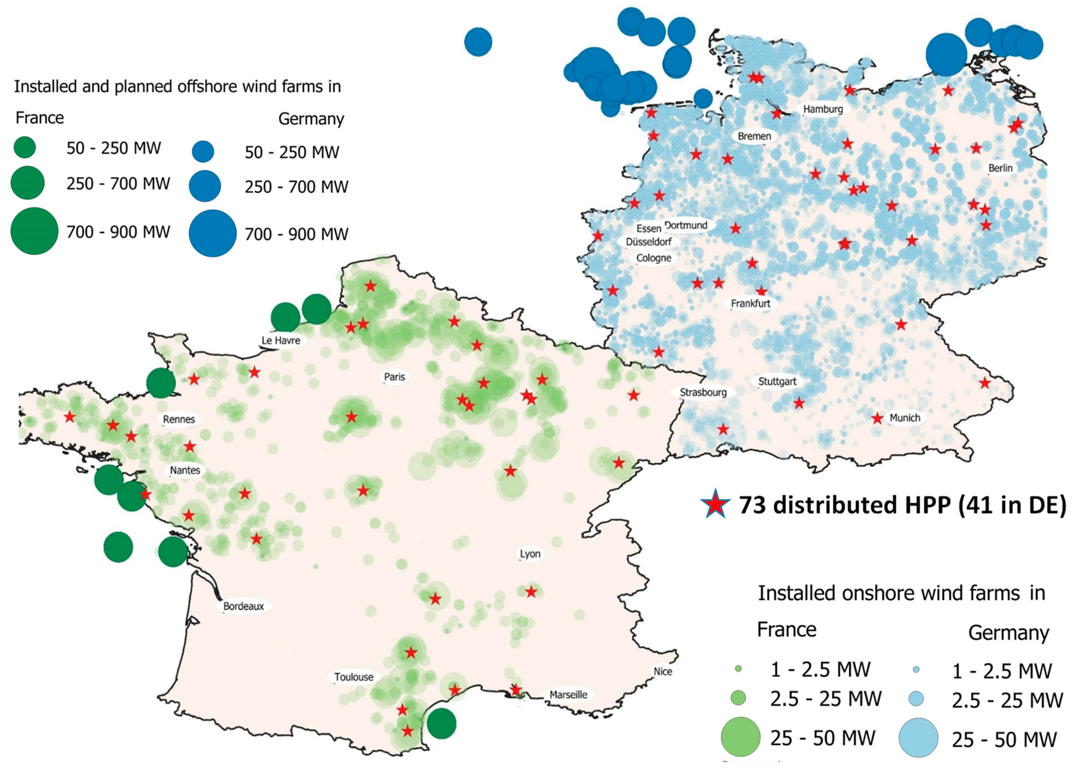
Finally, taking into account two different clustering methods (as defined by Equations (2) and (3)), two scenarios corresponding to different distribution of production capacities are developed, corresponding to centralized production and distributed production Figure 1.
In the sensitivity analysis, production cost was taken into account and was calculated using Equation (4), including different electricity costs associated to France and Germany depending on the location of the hydrogen production plant and the capacities, as defined by the clustering method. For both countries, correspondence has to be found between the annual electrical demand and the plant production size. Thus, Table 2 shows the corresponding maximum production plant size that could be run using the different bands. These band correspond to the consumption classification introduced in 2008 by the European Commission statistics to account for different annual consumption [48].
The different clustering methods gave two different scenarios that vary by the hydrogen production locations and distribution, as shown in Table 3.
4.3.2. Distribution Framework
All the demand projections are calculated per region defined by the population distribution. Each region corresponds to the NUTS-2 regions as defined by Eurostat [49,50]. First, the population of each NUTS-2 region [51] was taken and projected using the main scenario of population projection at a national level [52]. This allows forecasting the car park NUTS -2 regional numbers [53]. In fact, the main indicators used for population projection were fertility, death rate, age dynamic (share of more than 64 to less than 15), and, to a lesser extent, net immigration. Because of low fertility and death rates in the investigated countries, population projection is mainly driven by age dynamic, which has, in the case of France and Germany, a proportional increase between national and different regional levels. The same relation is noticed between the national and regional increase regarding the share of different young and elder populations that mainly influence the car park distribution.
In France and Germany, the need for transportation can be estimated by looking at the yearly average distance in km traveled by a person owning a private vehicle. This parameter is deduced from the number of populations and the car park, or the total traveled distance in million-person km. The main projection of European population growth is kept homogeneous [52], while the need for transportation in the coming 10 to 35 years was projected, taking into account historical trends. In fact, before the lockdown related to COVID-19, the need for transport was constant in the case of France, mainly due to central population distribution around Paris, where the population density reached its maximum. This yearly average distance traveled per capita is constant in France since 2000 [54], reaching its maximum value of 13,366 km per capita. For Germany, the yearly average distance traveled per capita is still increasing [54] because of regional distribution and a higher number of medium and high population density areas that favor commuting because of numerous job opportunities.
The car park prediction associated with the share of FCEV in transport can give an idea about the number of cars using conventional fuel that should be replaced. However, the penetration of the alternative fuels on the market is in an early commercialization phase, which makes it challenging to have an estimation about the share of new car technologies, mainly electric and hydrogen, in the car park projections. In fact, in terms of common policies, including France and Germany, hydrogen was not directly targeted, as the renewable energy directive pointed out a share of 6.8% of advanced renewable fuels by 2050 in the transport sector without any specific requirement [55]. This was revised and extended the share of renewable energy in transport to a mandatory minimum of 14%, targeting mainly biofuels [56], which opens perspectives for mainly battery electric and fuel cell electric vehicles.
For this study, a common scenario EU4 developed by the IEA for four European countries was used for the demand framework [57]. The share of FCEV is taken equally for the two countries to 2.4% by 2030 (or low penetration scenario case) and 28.5% by 2050 (or high penetration case). This scenario was chosen as it was more focused on the mobility sector and included France and Germany in the case studies. Another reason is that it allows a quantitative analysis of the demand at two years with a big penetration gap, which allows investigating the impact of a high increase of FCEV technology penetration. Recent scenarios matched to a certain extent the EU4 scenario, where the hydrogen council projected a share of 25% of hydrogen in passenger cars [58]. A recent outlook adjusted this share further down [59], to account for 14% of hydrogen in the transport sector in case of the same historical demand level (excluding 2020, where the demand for the transport sector is projected to decrease). However, the implication on the mobility sector is still unclear, with the shift of priority for road transport in recent policies to public transport and heavy carbonized vehicles [58,59,60].
The distribution nodes’ locations are based on the refueling stations. For that, all the primary refueling station geographical data [61], including in total more than 13,567 stations, are first sorted by country and NUTS-2 regions. For the distribution scenarios, the distribution location is set constant for both scenarios using the same clustering method, and only demand capacities are changed, corresponding to two years (or two penetration shares of fuel cell technology in the mobility sector).
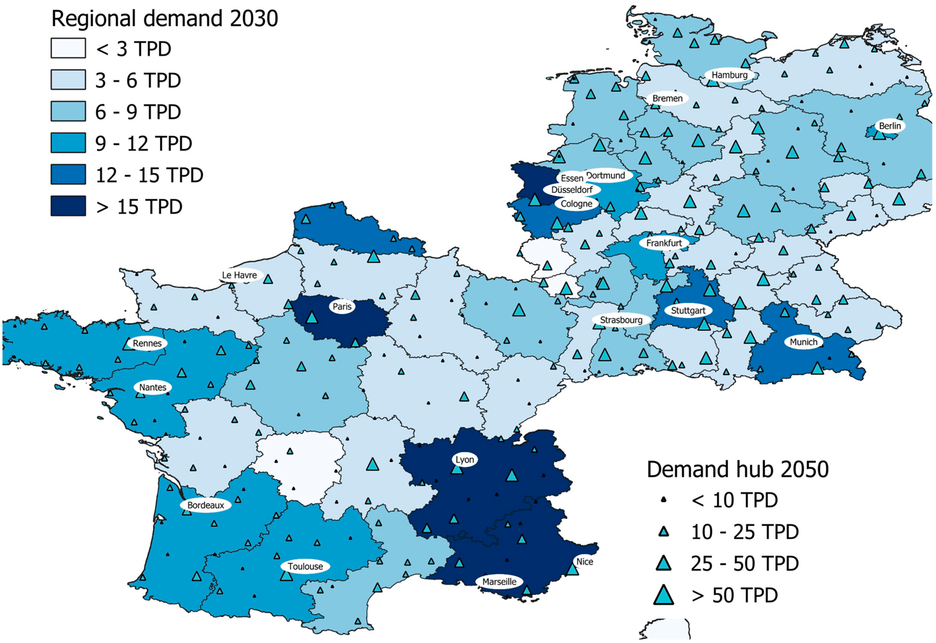
Figure 2 shows both scenarios, represented by regional demand for the year 2030 (at low penetration rate) and the distribution location and capacities for the year 2050 (at high penetration share).
4.3.3. Transport Framework
As the demand locations are fixed for the two demand scenarios, two road networks are defined, including distributed and localized production. In fact, only the road linking the different production and demand locations are kept, and four base case scenarios are defined, as shown in Table 4.
Three states are considered in hydrogen transport, namely, compressed gas CGH, liquid LH, and bound in a liquid organic carrier LOHC, and seven states of transport , accounting as well for five different pressure levels, ranging from 180 to 540 bar for compressed hydrogen.
All the cost parameters associated to storage and transport are calculated based on a quantitative analysis review of different storage and transport technology. The costs vary depending on the state of aggregation, which includes the tube trailer costs that are summarized in Table 5. Other costs common to the different states included cabin and undercarriage truck cost [62].
The transformation cost, based on different investment costs and energy requirements for compression, liquefaction process work, hydrogenation, and dehydrogenation, are modeled based on the literature review, developed models, and simulation to investigate the energy needs associated with each transformation [28,29].
As transformation between different states of transport at the storage node is allowed, the energy requirement from the initial state has to be adapted to different states of aggregation. The system work is considered null if the transformation is gaining work (for example, when we go from a high-pressure level to a lower one). Otherwise, the total work to transform hydrogen to a transport state is considered as a process work that uses hydrogen at an initial state at the hydrogen feed-in conditions. Thus, pre-work is needed to bring the hydrogen from atmospheric pressure to the feed-in state , and the work between and is then calculated from the total process and a pre-process (the same methodology can be adapted for instance to liquefaction work with pre-compression [63]).
This allows to calculate the transformation work between different processes, the initial one, , and the transport one, , taking into account the corresponding ideal work, and , and the different process efficiencies, and , as expressed in Equation (10):
Then, a technical assessment was performed to investigate and define the parameters associated with truck transportation, mainly including the number of trucks and the number of roundtrips specific to each transport state. Finally, the technical assessment is associated with an economic one to define the different cost parameters associated with the capital investment of the different transformation and storage plants as well as those associated with the use of truck transportation [30,62].
5. Results and Discussion
The results section presents, in the first part, the general results, where the impact of hydrogen demand and hydrogen production distribution on the transportation cost and technology is investigated. In the second part, the results of the sensitivity analysis are presented, including the impact of the production cost, and the modeling approach.
5.1. General Cost Results
The results show that demand is the main driver compared to production distribution, which has a lower impact on the cost. The results showed that for the base case scenarios and optimization method, compressed hydrogen gas is used: low to medium compression at low penetration scenarios and high compression at higher-penetration scenarios.
5.1.1. Scenarios Results
Concerning the demand scenario impact, the general results in Table 6 show that low demand scenarios (S1, S3) corresponding to the year 2030 have the lowest infrastructure deployment cost for France and Germany, while the increase of the demand in 2050 (S2, S4) increases the infrastructure cost considerably.
Concerning the production scenario impact, the general results show that the scenarios with distributed production plants (S1, S2) have a lower infrastructure cost compared to the centralized one (S3, S4).
When it comes to the transport technology, at low demand scenarios, most hydrogen is transported using low and medium pressure CGH for distributed production (S1) and using high pressure CGH for centralized production (S3). The increase of the demand in 2050 increases the flow transported between the different nodes, and applies the use of compressed gas at high-pressure level. In the case of centralized production, LOHC started to be used to balance the cost related to transportation.
As hydrogen transportation cost and technology are mainly impacted by the demand scenarios, S1 and S2, with distributed production, are chosen to show how the hydrogen is transported.
5.1.2. Flow Distribution
An analysis of the regions with the highest demand allows focusing on three main regions as presented in Figure 3:
- Northwestern Germany (NW), mainly North Rhine-Westphalia, with six main distribution locations;
- North of France (NF), mainly Île-de-France, with three main distribution locations;
- The region close to the border (BOR) between the two countries, with two main distribution locations.
In the NW region, the demand is satisfied by local production in 2030: the production plant P19 west of Düsseldorf covers both D5 and D2 demand, while P14 south of Bonn covers D3 demand. Meanwhile, D9 and D10 are linked to P13 and P18, respectively. The only exception is the hub demand D11, which exports hydrogen from the south of Germany at the French Border P9 (Figure 3). By 2050, the demand exceeds the regional production capacity, and hydrogen has to be exported from the production plant P17 in the north of Germany and from P15 and P16 located in east Germany. Moreover, the increase of the demand at the border also pushes the hydrogen to flow from north and east to south and west; thus, D11 is no longer exporting hydrogen from the south of Germany.
In the NF region, the wind potential is high, and the main hydrogen production allows covering the region’s demand. In the center of the region, the distribution hubs D1 and D4 are supplied using one production point P6 located east in 2030, while D12, located in the north, has its hydrogen transported from P20 only. The increase of the demand by 2050 impacts the central region as P6 alone cannot cover the demand in D1 and D4 anymore, and hydrogen also has to be transported from P1 south, P2 north, P4, and P5 west.
In the BOR region, mainly no exchange at the border happens in 2030. On the one hand, P7 and P8 allow the supply of all the distribution on the French side of the border. On the other hand, P9 and P10 are used to cover the demand on the German side of the border, including the main distribution hubs D7 and D8, and two minor demand hubs in France. By 2050, the increase of demand allows hydrogen to circulate from the French to the German border. In fact, D8 absorbs all the production from P9 and hydrogen has to be exported from France to cover the demand at D7 and all the hubs in the German side close to the border.
Concerning the flow in 2030, all the hydrogen transported to the main demand hubs does not exceed 50 TPD, while it reaches more than 100 TPD by 2050. On exception is D1, with the highest demand in the region of Paris, where demand exceeds 50 TPD in 2030.
5.2. Sensitivity Analysis
The model analysis allows investigating the transport and storage technology when optimizing hydrogen flow between fixed production and demand locations and capacities. However, the cost of the total supply chain also includes the production cost and the distribution cost. Therefore, it is legitimate to question the validity of the results when including other supply chain costs, since the same four scenarios (S1, S2, S3, S4) were simulated, including, the production cost in the scenario framework (Sp1, Sp2, Sp3, Sp4).
Then, the eight scenarios were simulated using a dynamic optimization method [30,62], which takes into account the daily storage option, to investigate the impact of the cost optimization method on the results.
5.2.1. Cost Analysis
Table 7 shows the cost results for the different scenarios including the production cost and using two optimization methods corresponding to the standard one with the technical and cost assessment calculated annually (optimization 1), and the dynamic one with a daily storage flexibility (optimization 2).
Introducing the production cost impacts the hydrogen flow that is transported not only with respect to the distance from the production plant but also with respect to the production cost. This change in priority increases the total distance and the flow of hydrogen transported at low demand scenarios, which results in higher transportation cost. The costs increase significantly for low demand scenarios, i.e., by 58% on average, compared to the scenarios without production cost constrains S1 and S3 to the scenarios with production cost constraints Sp1 and Sp3.
These results would have been expected as well at higher demand scenarios, but because of limited production capacities, the flow that could be transported from production plants with lower cost is restrained. This applies a difference lower than 2% between the scenarios at high penetration of hydrogen with and without production of an average.
Concerning the calculation method, low demand scenarios (S1, Sp1, S3, and Sp3) are mainly affected using the second optimization, as a cost reduction averaging 39 M€ is achieved. This translates in a reduction of the cost per total flow transported and stored by 0.08 €/kg. The dynamic model benefits mainly the hydrogen flow transported at low demand, which explains the results obtained. Thus, at a higher demand in 2050, the achieved cost reduction using the second optimization is minimal, and even marginal when comparing the cost rates.
5.2.2. Flow and Transport Distance Sensitivity Analysis
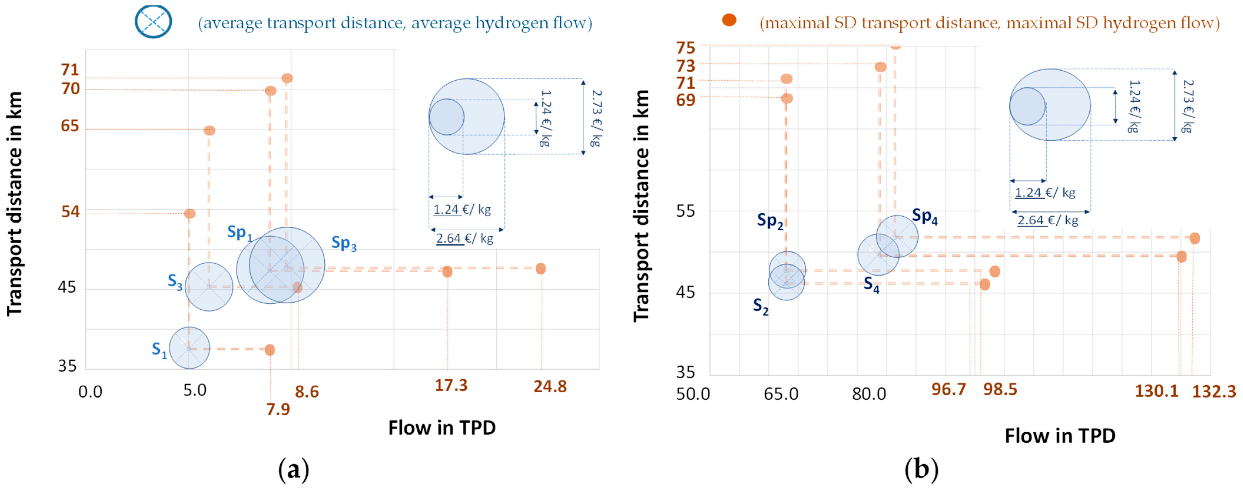
The cost differences between the different scenarios are mainly impacted by the flow transported and the transport distance between intermediate storage nodes. Thus, the average transport distance and the average hydrogen flow are presented by a circle with a radius proportional to the cost rate in Figure 4. The maximum standard deviation (SD) associated to the two parameters of the different scenarios are presented as well to show the distribution of the 34.1% values above the means.
Figure 4 shows that the cost increase can be explained by both an increase of the hydrogen flow and an increase of the distances between the intermediate storage. However, the effect of each parameter depends on the demand capacities, and the production cost and capacity constraints.
In 2030, for low demand scenarios (Figure 4a), the maximum transport distance SD varies with the number of the hydrogen production plants, as the lowest maximum SD of 54 km corresponds to the scenario with the highest HPP S1 in contrast to S3. The results also show that the increase of the cost in Sp1 and Sp3 comes mainly from the increase of the transported flow as maximal standard deviation (SD) increases by 119% and 188%, respectively. In fact, adding the production cost as constrain forces the demand to be fueled from production plants with lowest cost, which increases not only the distance ranges but also the transported and intermediate stored flow.
In 2050, for high demand scenarios (Figure 4b), Sp2 and Sp4 are not only constrained by the production cost, but also by the production capacities because of higher demand. Thus, the maximal standard deviation (SD) increases by less than 2% from S2 and S4, which translates to lower cost variations.
The impact of the transport distance can be seen in the cost variation between the scenarios. Thus, at low demand, a significant difference in the maximum transport distance SD ranging between 54 and 71 km results in a bigger disparity between the scenarios costs. In contrast, in 2050, the cost variation between the scenarios is marginal with regards to the maximum transport distance SD, which ranges between 69 and 75 km.
The results also show the dependency between the production and the demand scenarios. In fact, the choice of the production scenario affects the average transport distance and hydrogen flow, as the increase of the number of production plants decreases the transport distance ranges over which hydrogen is transported while decreasing the hydrogen flow because there are more accessible production sites. Simultaneously, increasing the demand scenarios from 2030 to 2050 increases the hydrogen flow, and because of the limited number of production plants, this increases the transport distance, as more hydrogen has to be transported from remote nodes.
5.2.3. Transport and Storage Technology Analysis
Table 8 shows the impact of the sensitivity analysis on the transport and storage technology used.
The results show that at a low demand (S1, Sp1, S3 and Sp3), using the second optimization allows the improvement of the infrastructure cost by using LOHC storage and transport, which shows more daily flexibility. Thus, for all scenarios, a share of low and high pressure CGH is replaced by LOHC, while medium pressure CGH maintains its share.
Concerning the results at high hydrogen penetration (S2, Sp2, S4, and Sp4), the results showed a small variation between the costs using standard and dynamic optimization. However, concerning the share of different transport states, the results showed a big variation for the LOHC share, but with a lower cost impact.
6. Conclusions
Hydrogen as an energy vector represents an alternative to conventional fuel in order to solve the problems related to the increase of greenhouse gas emissions. Nonetheless, the complexity of hydrogen transport restrains the deployment of adequate infrastructure at the national and European levels and restrains investment only to regional projects. Therefore, this article aims to discuss the optimal solutions that could be used to transport and store hydrogen to reduce the cost associated with the infrastructure deployment for mobility. These solutions are investigated for different production and demand scenarios in France and Germany.
The general modeling approach aims to link production and demand nodes following the road infrastructure and using different transportation cost functions corresponding to seven states of transport. Thus, the model output for each edge gives the optimum capacity transported by each state and then the minimum cost of the entire network. The model uses as a framework the road infrastructure and the hydrogen production and demand scenarios, assuming hydrogen production from wind power projections and a demand driven by mobility.
Besides comparing different transport and hydrogen storage options, the study aims to minimize the annual cost using two optimization methods giving a guideline about the technologies that could be used at different flow, transport distance ranges, production, and demand scenarios. Thus, low to medium compressed hydrogen with lower energy requirements are promoted at low demand. Meanwhile, at higher demand, the total transport distance traveled to deliver hydrogen could be reduced by increasing the capacity transported by every single truck, and thus, promoting higher pressure rates of compressed hydrogen. The use of a different modeling approach underlines how the choice of transport and storage technology is important in low-demand scenarios.
Sixteen scenarios in total were analyzed, which differed by production distribution and cost, hydrogen demand, and modeling method. The results showed a dependency between the model frameworks, mainly production and demand scenarios. Increasing the production plant distribution decreases the transport distance ranges and the hydrogen flow because of more accessible production sites. Simultaneously, increasing the hydrogen demand increases the hydrogen flow and the transport distance, as more hydrogen has to be transported from remote nodes.
The demand change had the highest impact, and the main distribution nodes were located in three main regions: western Germany around North Rhine-Westphalia, the north of France, including the Île-de-France region, and the border between the two countries.
In western Germany, the demand is satisfied by local production in 2030, while regional import is needed to satisfy the demand in 2050, mainly from the north and west of Germany. The north of France has great wind potential, and none of the hydrogen production for both years is imported from surrounding regions. However, up to four production plants are needed to cover, for instance, the main demand hub located in the northwest of Paris. Finally, marginal exchange at the border is noticeable in 2030, while more than 10% of hydrogen demand in 2050 at the German side border is covered via import from France.
Concerning production, the scenarios with distributed production plants have a lower infrastructure cost compared to the centralized one, and low demand scenarios are more impacted when including the cost of hydrogen production as the total cost increases because of an increase in the maximum flow and distance standard deviations by 16 TPD and 6 km, respectively.
Finally, the same conclusion can be made with regards to the impact of the optimization method choice, as low-demand scenarios are mainly impacted using dynamic optimization by achieving a cost reduction averaging 39 M€ compared to standard optimization.
In fact, at low demand, using dynamic optimization improvement of the infrastructure cost is achieved by using liquid organic hydrogen carrier storage and transport, which allows for more daily flexibility. Thus, for all low demand scenarios, a share of compressed gas is replaced with LOHC. In contrast, a significant variation for the LOHC share was noticeable at high hydrogen penetration; however, this had a small cost impact. Thus, a choice of adequate technology to transport hydrogen is more critical at the early stage of infrastructure deployment.
Author Contributions
Conceptualization, A.L., C.W. and D.D.; methodology, A.L.; validation, A.L., C.W. and D.D.; investigation, A.L.; data curation, A.L.; writing—original draft preparation, A.L.; writing—review and editing, A.L., C.W. and D.D.; visualization, A.L.; supervision, C.W. and D.D. All authors have read and agreed to the published version of the manuscript.
Funding
This research received no external funding.
Conflicts of Interest
The authors declare no conflict of interest.
Nomenclature
| Installed capacity for a technology in 2016 | |
| Location in a given country framework | |
| Average capacity factor associated to a technology , in a country | |
| Projected wind farm generation | |
| National generation increase depending on the technology | |
| Total hydrogen production | |
| Higher heating value | |
| Clustering of the wind farms by location | |
| Coordinates associated to a location | |
| Levelized cost of producing hydrogen | |
| Electricity price | |
| Regional population distribution for 2016 | |
| Regional population projection | |
| Regional car park distribution for 2016 | |
| Yearly average travelled distance per capita owning a private vehicle | |
| Share of FCEV in mobility | |
| FCEV driving range | |
| Regional hydrogen demand projection | |
| Hydrogen demand projection of the distribution hub located in | |
| Clustering of the refueling stations by location | |
| Production and demand nodes | |
| Edge linking two nodes and | |
| Flow transported between and at a transport state | |
| Levelized cost of transforming hydrogen from a state to | |
| Levelized cost of storing hydrogen at a state | |
| Levelized cost of transporting hydrogen using a state | |
| Minimum transportation cost function from an initial state to a transport state | |
| Total hydrogen flow between nodes and | |
| Optimum flow the production and the demand nodes | |
| , | Production and demand node, respectively |
| Transport distance between the two nodes and | |
| Intersection of the edge and all the hydrogen flows linking the production and demand nodes | |
| Group of hydrogen transport states | |
| Minimum transportation cost function from the production state to a transport state | |
| Minimum transportation cost function from the transport state to the final conditions | |
| Electricity prices associated to France for the reference year 2016 | |
| Electricity prices associated to Germany for the reference year 2016 | |
| Base case scenarios for infrastructure deployment cost calculation | |
| Scenario including distributed green hydrogen production | |
| Scenario including localized green hydrogen production | |
| Work associated to hydrogen transformation from a state to | |
| Ideal transformation work associated to a process | |
| Process efficiency | |
| Scenarios including production cost |
Acronyms
| Band | |
| CGH | Compressed hydrogen |
| EU4 | Scenario developed by IEA for hydrogen mobility |
| FCEV | Fuel cell electric vehicle |
| HPP | Hydrogen production plants |
| IEA | International energy agency |
| LH | Liquid hydrogen |
| LOHC | Liquid organic hydrogen carrier |
| NREL | National renewable energy laboratory |
| NUTS | Nomenclature of Territorial Units for Statistics |
| PEM | Proton exchange membrane |
| RES | Renewable energy sources |
| SoT | State of hydrogen transport |
References
- Helm, D. The Environmental Impacts of the Coronavirus. Environ. Resour. Econ. 2020, 76, 21–38. [Google Scholar] [CrossRef] [PubMed]
- EU. Energy in Figures, Statistical Pocketbook 2019; European Commission: Luxemburg, 2019. [Google Scholar]
- Amos, W.A. Costs of Storing and Transporting Hydrogen; National Renewable Energy Laboratory: Golden, CO, USA, 1999. [Google Scholar]
- Yang, C.; Ogden, J.M. Determining the lowest-cost hydrogen delivery mode. Int. J. Hydrogen Energy 2007, 32, 268–286. [Google Scholar] [CrossRef] [Green Version]
- Simbeck, D.; Chang, E. Hydrogen Supply: Cost Estimate for Hydrogen Pathways–Scoping Analysis; National Renewable Energy Laboratory: Mountain View, CA, USA, 2002. [Google Scholar]
- Council, N.R. The Hydrogen Economy: Opportunities, Costs, Barriers, and R&D Needs; National Academies Press: Washington, DC, USA, 2004. [Google Scholar]
- Brey, J.; Carazo, A.F.; Brey, R. Using AHP and binary integer programming to optimize the initial distribution of hydrogen infrastructures in Andalusia. Int. J. Hydrogen Energy 2012, 37, 5372–5384. [Google Scholar] [CrossRef]
- Reuß, M.; Grube, T.; Robinius, M.; Preuster, P.; Wasserscheid, P.; Stolten, D. Seasonal storage and alternative carriers: A flexible hydrogen supply chain model. Appl. Energy 2017, 200, 290–302. [Google Scholar] [CrossRef]
- Xu, X.; Xu, B.; Dong, J.; Liu, X. Near-term analysis of a roll-out strategy to introduce fuel cell vehicles and hydrogen stations in Shenzhen China. Appl. Energy 2017, 196, 229–237. [Google Scholar] [CrossRef]
- Lin, Z.; Chen, C.-W.; Ogden, J.; Fan, Y. The least-cost hydrogen for Southern California. Int. J. Hydrogen Energy 2008, 33, 3009–3014. [Google Scholar] [CrossRef]
- Anex, R.P.; Aden, A.; Kazi, F.K.; Fortman, J.; Swanson, R.M.; Wright, M.M.; Satrio, J.A.; Brown, R.C.; Daugaard, D.E.; Platon, A.; et al. Techno-economic comparison of biomass-to-transportation fuels via pyrolysis, gasification, and biochemical pathways. Fuel 2010, 89, S29–S35. [Google Scholar] [CrossRef]
- Almansoori, A.; Shah, N. Design and Operation of a Future Hydrogen Supply Chain. Chem. Eng. Res. Des. 2006, 84, 423–438. [Google Scholar] [CrossRef]
- Almansoori, A.; Shah, N. Design and operation of a future hydrogen supply chain: Multi-period model. Int. J. Hydrogen Energy 2009, 34, 7883–7897. [Google Scholar] [CrossRef]
- Han, J.-H.; Ryu, J.-H.; Lee, I.-B. Modeling the operation of hydrogen supply networks considering facility location. Int. J. Hydrogen Energy 2012, 37, 5328–5346. [Google Scholar] [CrossRef]
- Hwangbo, S.; Lee, S.; Yoo, C. Optimal network design of hydrogen production by integrated utility and biogas supply networks. Appl. Energy 2017, 208, 195–209. [Google Scholar] [CrossRef]
- Kim, M.; Kim, J. Optimization model for the design and analysis of an integrated renewable hydrogen supply (IRHS) system: Application to Korea’s hydrogen economy. Int. J. Hydrogen Energy 2016, 41, 16613–16626. [Google Scholar] [CrossRef]
- Moreno-Benito, M.; Agnolucci, P.; Papageorgiou, L.G. Towards a sustainable hydrogen economy: Optimisation-based framework for hydrogen infrastructure development. Comput. Chem. Eng. 2017, 102, 110–127. [Google Scholar] [CrossRef] [Green Version]
- Nunes, P.; Oliveira, F.; Hamacher, S.; Almansoori, A. Design of a hydrogen supply chain with uncertainty. Int. J. Hydrogen Energy 2015, 40, 16408–16418. [Google Scholar] [CrossRef]
- Woo, Y.-B.; Cho, S.; Kim, J.; Kim, B.S. Optimization-based approach for strategic design and operation of a biomass-to-hydrogen supply chain. Int. J. Hydrogen Energy 2016, 41, 5405–5418. [Google Scholar] [CrossRef]
- Maroufmashat, A.; Fowler, M.; Khavas, S.S.; Elkamel, A.; Roshandel, R.; Hajimiragha, A.H. Mixed integer linear programing based approach for optimal planning and operation of a smart urban energy network to support the hydrogen economy. Int. J. Hydrogen Energy 2016, 41, 7700–7716. [Google Scholar] [CrossRef]
- Li, Z.; Gao, D.; Chang, L.; Liu, P.; Pistikopoulos, E.N. Hydrogen infrastructure design and optimization: A case study of China. Int. J. Hydrogen Energy 2008, 33, 5275–5286. [Google Scholar] [CrossRef]
- Han, J.-H.; Ryu, J.-H.; Lee, I.-B. Multi-objective optimization design of hydrogen infrastructures simultaneously considering economic cost, safety and CO2 emission. Chem. Eng. Res. Des. 2013, 91, 1427–1439. [Google Scholar] [CrossRef]
- Hwangbo, S.; Nam, K.; Han, J.; Lee, I.-B.; Yoo, C. Integrated hydrogen supply networks for waste biogas upgrading and hybrid carbon-hydrogen pinch analysis under hydrogen demand uncertainty. Appl. Therm. Eng. 2018, 140, 386–397. [Google Scholar] [CrossRef]
- André, J.; Auray, S.; De Wolf, D.; Memmah, M.-M.; Simonnet, A. Time development of new hydrogen transmission pipeline networks for France. Int. J. Hydrogen Energy 2014, 39, 10323–10337. [Google Scholar] [CrossRef] [Green Version]
- Almaraz, S.D.-L.; Azzaro-Pantel, C.; Montastruc, L.; Boix, M. Deployment of a hydrogen supply chain by multi-objective/multi-period optimisation at regional and national scales. Chem. Eng. Res. Des. 2015, 104, 11–31. [Google Scholar] [CrossRef]
- Stephens-Romero, S.D.; Brown, T.M.; Kang, J.E.; Recker, W.W.; Samuelsen, S. Systematic planning to optimize investments in hydrogen infrastructure deployment. Int. J. Hydrogen Energy 2010, 35, 4652–4667. [Google Scholar] [CrossRef] [Green Version]
- Almaraz, S.D.-L.; Azzaro-Pantel, C.; Montastruc, L.; Domenech, S. Hydrogen supply chain optimization for deployment scenarios in the Midi-Pyrénées region, France. Int. J. Hydrogen Energy 2014, 39, 11831–11845. [Google Scholar] [CrossRef] [Green Version]
- Lahnaoui, A.; Wulf, C.; Dalmazzone, D. Impact of the optimization method on reducing the infrastructure cost of hydrogen transported at different states of aggregation. In Proceedings of the International Conference on Applied Energy 2019, Västerås, Sweden, 12–15 August 2019. [Google Scholar]
- Lahnaoui, A.; Wulf, C.; Dalmazzone, D. Impact of the optimization method on the cost and the choice of hydrogen transport state of aggregation. In Proceedings of the 2019 International Conference on Applied Energy, ICAE 2019, Västerås, Sweden, 12–15 August 2019. [Google Scholar]
- Heinrichs, H.U.; Wulf, C.; Heinrichs, H.; Dalmazzone, D. Optimizing hydrogen transportation system for mobility by minimizing the cost of transportation via compressed gas truck in North Rhine-Westphalia. Appl. Energy 2018, 223, 317–328. [Google Scholar] [CrossRef]
- Schmidt, O.; Gambhir, A.; Staffell, I.; Hawkes, A.; Nelson, J.; Few, S. Future cost and performance of water electrolysis: An expert elicitation study. Int. J. Hydrogen Energy 2017, 42, 30470–30492. [Google Scholar] [CrossRef]
- NREL. H2A: Hydrogen Analysis Production Models; Version 3.101; NREL: Golden, CO, USA, 2015.
- Eurostat. Archive: Statistics on Regional Population Projections; European Commission: Luxembourg, 2019. [Google Scholar]
- Stolten, D. Hydrogen Science and Engineering: Materials, Processes, Systems and Technology, 2 Volume Set; John Wiley & Sons: Hoboken, NJ, USA, 2016. [Google Scholar]
- IEA. The Future of Hydrogen, Seizing Today’s Opportunities; International Energy Agency: Paris, France, 2019. [Google Scholar]
- Gouv. Plan Climat; Le ministère de la Transition Écologique et Solidaire: Paris, France, 2017.
- Afhypac. L’hydrogène: Défi National, Enjeux Territoriaux; Association Français pour l’hydrogène et les Piles Combustibles: Paris, France, 2018. [Google Scholar]
- Afhypac. Développons l’Hydrogène Pour l’économie Française; Association Français pour L’hydrogène et les Piles Combustibles: Paris, France, 2018. [Google Scholar]
- Jones, D.; Sakhel, A.; Buck, M.; Graichen, P. The European Power Sector in 2018, Up-To-Date Analysis on the Electricity Transition; Sandbag: London, UK; Agora Energiewende: Berlin, Germany, 2019. [Google Scholar]
- Agora. Energiewende 2030: The Big Picture; Agora Energiewende: Berlin, Germany, 2018. [Google Scholar]
- Agora. Transforming the Transport Sector: 12 Insights into the Verkehrswende; Agora Verkehrswende: Berlin, Germany, 2017. [Google Scholar]
- Eolienne, F.E. La Transition Énergétique. Available online: http://fee.asso.fr/politique-de-leolien/la-transition-energetique/ (accessed on 5 January 2018).
- WindEurope. Wind in Power 2017; Annual Combined Onshore and Offshore Wind Energy Statistics: Brussels, Belgium, 2018. [Google Scholar]
- OPSD. Renewable Power Plants DE. Available online: https://data.open-power-system-data.org/renewable_power_plants/ (accessed on 29 May 2018).
- Power, T.W. Total Installed Capacity by Country. Available online: http://www.thewindpower.net/country_list_en.php (accessed on 5 September 2017).
- WindPower. Datasets Countries. 2017. Available online: https://www.thewindpower.net/windfarms_list_en.php (accessed on 5 September 2017).
- OPSD. Renewable Power Plants. Available online: https://doi.org/10.25832/renewable_power_plants/2020-08-25 (accessed on 26 January 2018).
- Eurostat. Energy Statistics—Electricity Prices for Domestic and Industrial Consumers, Price Components. Available online: https://ec.europa.eu/eurostat/cache/metadata/en/nrg_pc_204_esms.htm (accessed on 7 October 2019).
- Eurostat. NUTS Regions in Germany. Available online: http://ec.europa.eu/eurostat/documents/345175/7451602/nuts-map-DE.pdf (accessed on 26 January 2018).
- Eurostat. NUTS Regions in France. Available online: http://ec.europa.eu/eurostat/documents/345175/7451602/nuts-map-FR.pdf (accessed on 26 January 2018).
- Eurostat. Population on 1 January by NUTS 2 Region. Available online: http://ec.europa.eu/eurostat/tgm/table.do?tab=table&init=1&language=en&pcode=tgs00096&plugin=1 (accessed on 12 June 2018).
- Eurostat. Population Projections Data. Available online: http://ec.europa.eu/eurostat/web/population-demography-migration-projections/population-projections-data (accessed on 7 May 2017).
- Eurostat. Stock of Vehicles by Category and NUTS 2 Regions. Available online: http://appsso.eurostat.ec.europa.eu/nui/show.do?dataset=tran_r_vehst&lang=en (accessed on 7 May 2018).
- Eurostat. Passenger Road Transport on National Territory, by Type of Vehicles Registered in the Reporting Country. Available online: http://ec.europa.eu/eurostat/web/transport/data/database (accessed on 7 May 2017).
- European Commission. Renewable Energy Directive; 2009/28/EC, Union; European Commission: Brussels, Belgium, 2009; Volume 2009/28/EC. [Google Scholar]
- European Commission. Revised Renewable Energy Directive; European Commission: Brussels, Belgium, 2018. [Google Scholar]
- IEA. Technology Roadmap: Hydrogen and Fuel Cells; International Energy Agency: Paris, France, 2015. [Google Scholar]
- Hydrogen Council. Hydrogen Scaling Up, a Sustainable Pathway for the Global Energy Transition; Hydrogen Council: Brussels, Belgium, 2017. [Google Scholar]
- FCH JU. Hydrogen Roadmap Europe; FCH JU: Bruxelles, Belgium, 2019. [Google Scholar]
- European Comission. COM(2020) 301, A Hydrogen Strategy for a Climate-Neutral Europe; European Comission: Brussels, Belgium, 2020. [Google Scholar]
- Essofuelfinder. Available online: https://wholesalefuels.esso.de/de-DE/ (accessed on 9 December 2017).
- Lahnaoui, A.; Wulf, C.; Heinrichs, H.; Dalmazzone, D. Optimizing hydrogen transportation system for mobility via compressed hydrogen trucks. Int. J. Hydrogen Energy 2019, 44, 19302–19312. [Google Scholar] [CrossRef]
- Berstad, D.; Stang, J.H.; Neksa, P. Comparison criteria for large-scale hydrogen liquefaction processes. Int. J. Hydrogen Energy 2009, 34, 1560–1568. [Google Scholar] [CrossRef]
Figure 1.
Location of wind farms and distributed hydrogen production plants (HPP). Changing the clustering methodology form narrow to wider allows defining a localized scenario with 22 HPP (12 in Germany).
Figure 1.
Location of wind farms and distributed hydrogen production plants (HPP). Changing the clustering methodology form narrow to wider allows defining a localized scenario with 22 HPP (12 in Germany).

Figure 2.
Regional demand for 2030 and demand hub capacities for 2050.

Figure 3.
Hydrogen transported in and at high demand regions.
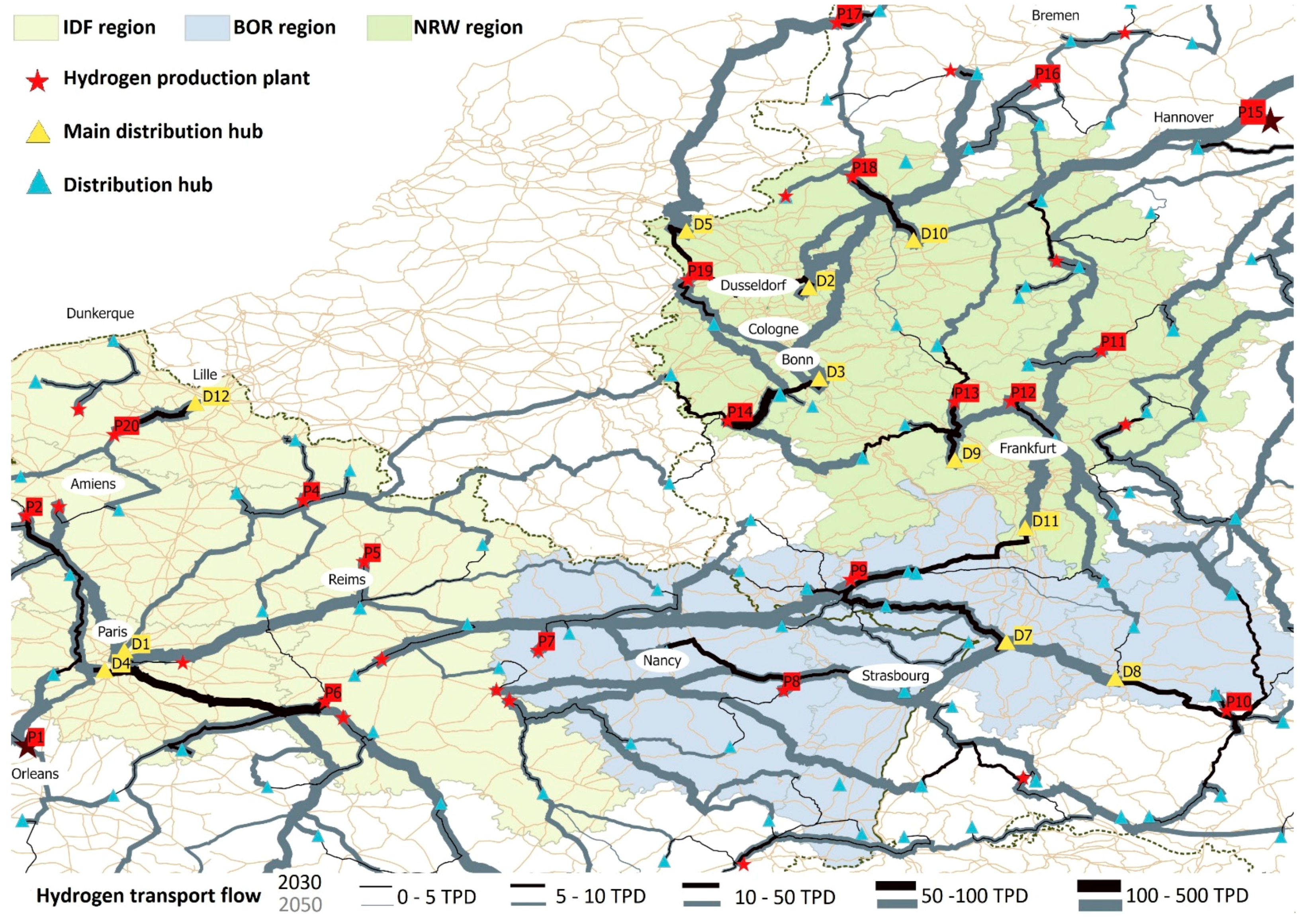
Figure 4.
Average and maximum standard deviation (SD) of the transport distance and flow for low demand (a) and high demand scenarios (b).
Figure 4.
Average and maximum standard deviation (SD) of the transport distance and flow for low demand (a) and high demand scenarios (b).


Table 1.
Wind dataset that contains geographical information.
| Data | France | Germany | ||
|---|---|---|---|---|
| Onshore | Offshore | Onshore | Offshore | |
| Data set of installed wind farms | 13.57 GW | - | 50.42 GW | 5.32 GW |
| Data set of planned wind farms | - | 4.05 GW | - | 8.60 GW |
Table 2.
Maximum production plant (HPP) size for different non-household consumers (band).
| Band Classification | Below IC | ID | IE | IF | IG |
|---|---|---|---|---|---|
| Maximum HPP size in TPD 1 | 1.25 | 12.3 | 42.0 | 97.2 | 200 |
| in €/kWh | 0.111 | 0.092 | 0.077 | 0.064 | 0.055 |
| in €/kWh | 0.197 | 0.170 | 0.136 | 0.118 | 0.110 |
1 A correspondence was calculated between production capacity in TPD and electricity consumption in MWh for the different consumption band introduced by EC Eurostat [48].
Table 3.
Maximum production plant (HPP) size for different non-household consumers (band).
| Production | Distributed | Centralized | ||
|---|---|---|---|---|
| Country | France | Germany | France | Germany |
| Number of production plants | 32 | 41 | 9 | 12 |
| Minimum in €/kg | 2.32 | 3.88 | 2.32 | 3.88 |
| Maximum in €/kg | 3.17 | 6.87 | 2.38 | 4.06 |
Table 4.
Base case scenarios for hydrogen transport and storage in France and Germany.
| Scenario | Demand Penetration | Road Network | ||
|---|---|---|---|---|
| Low (2030) | High (2050) | CS11 | CS22 | |
| S1 | X | X | ||
| S2 | X | X | ||
| S3 | X | X | ||
| S4 | X | X | ||
1CS1 includes 73 production plants (41 in Germany and 32 in France). 2 CS2 includes 22 production plants (12 in Germany and 10 in France).
Table 5.
Assumption for tube trailer used to store and transport from own calculation and sources [28,29,62].
| State of Aggregation (SoT) | CGH | LOHC | LH | ||||
|---|---|---|---|---|---|---|---|
| Storage pressure in bar | 180 | 250 | 350 | 500 | 540 | 1 | 1 |
| Index of SoT | 2 | 3 | 4 | 5 | 6 | 8 | 9 |
| Net truck capacity in kg | 350 | 668 | 885 | 1100 | 1230 | 1500 | 3600 |
| Tube trailer cost in K€ | 385 | 525 | 689 | 1057 | 1197 | 57 | 1732 |
Table 6.
Different scenarios results cost and transport technology.
| Infrastructure Cost in M€ | Transport Technologies Share %/km | |||||
|---|---|---|---|---|---|---|
| Compressed Gas | LOHC | Liquid | ||||
| Low | Medium | High | ||||
| S1 | 672 | 39.58 | 24.61 | 35.81 | 0.00 | 0 |
| S3 | 785 | 29.95 | 16.22 | 53.83 | 0.00 | 0 |
| S2 | 6649 | 0.46 | 2.83 | 96.58 | 0.13 | 0 |
| S4 | 7550 | 0.29 | 1.55 | 94.96 | 3.20 | 0 |
Table 7.
Sensitivity analysis of the cost in M€ and the corresponding cost per transported and stored hydrogen in €/kg.
Table 7.
Sensitivity analysis of the cost in M€ and the corresponding cost per transported and stored hydrogen in €/kg.
| Hydrogen Penetration | Low Demand | High Demand | |||||||
|---|---|---|---|---|---|---|---|---|---|
| Scenario | S1 | S3 | Sp1 | Sp3 | S2 | S4 | Sp2 | Sp4 | |
| Total cost in M€ | Optimization 1 | 672 | 785 | 1083 | 1221 | 6649 | 7550 | 6723 | 7637 |
| Optimization 2 | 634 | 746 | 1050 | 1178 | 6642 | 7546 | 6716 | 7633 | |
| Cost rate in €/kg | Optimization 1 | 1.50 | 1.76 | 2.42 | 2.73 | 1.24 | 1.41 | 1.25 | 1.42 |
| Optimization 2 | 1.42 | 1.67 | 2.35 | 2.64 | 1.24 | 1.40 | 1.25 | 1.42 | |
Table 8.
Sensitivity analysis of the share of transport technology per transported distance.
| Cost Optimization 1 | Cost Optimization 2 | |||||||||
|---|---|---|---|---|---|---|---|---|---|---|
| Compressed Gas | LOHC | Liquid | Compressed Gas | LOHC | Liquid | |||||
| Low | Medium | High | Low | Medium | High | |||||
| S1 | 39.58 | 24.61 | 35.81 | 0.00 | 0.00 | 29.27 | 24.61 | 35.81 | 6.56 | 0.00 |
| Sp1 | 24.58 | 12.99 | 62.43 | 0.00 | 0.00 | 18.43 | 12.99 | 62.43 | 6.15 | 0.00 |
| S2 | 0.46 | 2.83 | 96.58 | 0.13 | 0.00 | 0.05 | 0.00 | 60.57 | 39.43 | 0.00 |
| Sp2 | 1.16 | 2.54 | 94.88 | 1.42 | 0.00 | 0.00 | 0.00 | 54.94 | 45.06 | 0.00 |
| S3 | 29.95 | 16.22 | 53.83 | 0.00 | 0.00 | 21.91 | 16.22 | 55.59 | 6.29 | 0.00 |
| Sp3 | 21.79 | 9.74 | 68.42 | 0.05 | 0.00 | 13.79 | 9.74 | 68.52 | 7.95 | 0.00 |
| S4 | 0.29 | 1.55 | 94.96 | 3.20 | 0.00 | 0.00 | 0.00 | 44.01 | 55.99 | 0.00 |
| Sp4 | 0.70 | 2.34 | 93.81 | 3.16 | 0.00 | 0.00 | 0.00 | 56.76 | 43.24 | 0.00 |
Publisher’s Note: MDPI stays neutral with regard to jurisdictional claims in published maps and institutional affiliations. |
© 2021 by the authors. Licensee MDPI, Basel, Switzerland. This article is an open access article distributed under the terms and conditions of the Creative Commons Attribution (CC BY) license (http://creativecommons.org/licenses/by/4.0/).
Share and Cite
MDPI and ACS Style
Lahnaoui, A.; Wulf, C.; Dalmazzone, D. Optimization of Hydrogen Cost and Transport Technology in France and Germany for Various Production and Demand Scenarios. Energies 2021, 14, 744. https://doi.org/10.3390/en14030744
AMA Style
Lahnaoui A, Wulf C, Dalmazzone D. Optimization of Hydrogen Cost and Transport Technology in France and Germany for Various Production and Demand Scenarios. Energies. 2021; 14(3):744. https://doi.org/10.3390/en14030744
Chicago/Turabian StyleLahnaoui, Amin, Christina Wulf, and Didier Dalmazzone. 2021. "Optimization of Hydrogen Cost and Transport Technology in France and Germany for Various Production and Demand Scenarios" Energies 14, no. 3: 744. https://doi.org/10.3390/en14030744
Note that from the first issue of 2016, this journal uses article numbers instead of page numbers. See further details here.