Article

A Methodology for Provision of Frequency Stability in Operation Planning of Low Inertia Power Systems

1
Department of Automation and System Analysis, Institute of Power Engineering (IEn) Gdańsk Division, PL80-870 Gdańsk, Poland
2
ENEA–Department of Energy Technologies and Renewable Sources, 00196 Rome, Italy
3
FOSS Research Centre for Sustainable Energy, University of Cyprus, 1678 Nicosia, Cyprus
*
Author to whom correspondence should be addressed.
Energies 2021, 14(3), 737; https://doi.org/10.3390/en14030737
Submission received: 15 January 2021 / Revised: 27 January 2021 / Accepted: 27 January 2021 / Published: 31 January 2021

Abstract

:
Along with the increasing share of non-synchronous power sources, the inertia of power systems is being reduced, which can give rise to frequency containment problems should an outage of a generator or a power infeed happen. Low system inertia is eventually unavoidable, thus power system operators need to be prepared for this condition. This paper addresses the problem of low inertia in the power system from two different perspectives. At a system level, it proposes an operation planning methodology, which utilises a combination of power flow and dynamic simulation for calculation of existing inertia and, if need be, synthetic inertia (SI) to fulfil the security criterion of adequate rate of change of frequency (RoCoF). On a device level, it introduces a new concept for active power controller, which can be applied virtually to any power source with sufficient response time to create synthetic inertia. The methodology is demonstrated for a 24 h planning period, for which it proves to be effective. The performance of SI controller activated in a battery energy storage system (BESS) is positively validated using a real-time digital simulator (RTDS). Both proposals can effectively contribute to facilitating the operation of low inertia power systems.

Graphical Abstract

1. Introduction

1.1. Motivation

Following the EU goals for decarbonisation, ENTSO-E has anticipated three possible scenarios for the interconnected European grid of 2050 [1]. These scenarios foresee high levels of renewable energy resources (RES) in the overall generation mix, ranging from 69 to 82%, and in result high level of demand supply from renewables. The shift from traditional generation into more intermittent production based on wind and solar power sources will change how the system is operated. Transition to the generation and loads decoupled from the grid through converters will cause weakening of the systems’ ability to remain stable after significant disturbances, such as generator/load trip or system split [2,3], which has already been reported in countries with high RES penetration, such as Great Britain or Ireland [4]. In other words, as the amount of kinetic energy from the generators spinning masses lowers, the system becomes more prone to disturbances resulting in power imbalances, which leads to severe frequency deviations and a higher rate of change of frequency (RoCoF), reaching 6 Hz/s in extreme cases [3].
It is anticipated that in the future the variations in total system inertia will be much higher [5], both during the day, as hourly RES penetration can be 4–5 times greater than the average penetration [6] and during the year [7]. Situations in which equivalent system inertia will be as low as 1 s (compared to traditional 5–6 s) will pose severe threat to frequency stability. Therefore, system monitoring and system awareness become vital in order to predict these moments in such advance that necessary countermeasures can be prepared in the operation planning phase.
To avoid system collapse after a disturbance, it is essential to limit RoCoF, so that the remaining generators are not tripped by the under-frequency or RoCoF protection [8]. It is also of high importance to evade load shedding, as in the grids with high RES penetration (especially PV), a significant amount of generation is located in the distribution network and, therefore, could be switched off along with the load, resulting in further frequency decline. High RoCoF could also result in UFLS not being able to act sufficiently fast [3].
Several steps have already been undertaken to facilitate the transformation process. Firstly, the concept of synthetic inertia was introduced to the Grid Codes [9,10,11]. Additionally, several Implementation Guidance Documents dealing with RoCoF withstand capability [12], inertia in the system [8] and high penetration of inertia-less devices [6] were released by ENTSO-E. Some of these recommendations, such as increasing the activation threshold of RoCoF-triggered protection, are already being implemented [13,14], but in general, these documents are the prerequisites that need to be supplemented by proper tools and methodologies supporting the operation of the power system in low inertia conditions.

1.2. Overview of Available Countermeasures for Supporting Low Inertia

Both the researchers and the industry acknowledge the need for maintaining inertia, whether by synchronous or synthetic means, mainly in order to keep the RoCoF relay settings unchanged, as there are concerns about synchronous generators’ ability to withstand higher values of RoCoF due to the possible instability and a shorter lifetime [4,12]. A conservative view to address this issue, often expressed by transmission system operators (TSO), is to rely on conventional means such as synchronous compensators or “imported” system strength through the AC connections [6]. However, various countermeasures utilising non-synchronous power sources have also been proposed.
In particular, usage of different energy storage systems (ESS) for frequency support has been of increasing interest. Supercapacitors are fast-acting ESS, which can be used within fast frequency response (FFR) control schemes. While not capable of sustaining their power output for prolonged time, supercapacitors could be used for the initial frequency response, provided that they are backed by another source of active power to achieve frequency stability [15]. A battery energy storage system (BESS), on the other hand, in general, have appropriate dynamic properties for frequency support and can host various control schemes, such as variable droop [16] or specially designed energy management systems (EMS) that utilize inertial response [17]. A comprehensive comparison of alternative types of frequency support from inverter-connected devices, considering different triggers (frequency, RoCoF, time) as well as control schemes can be found in Ref. [4].
Before BESS became applicable to power system problems, wind turbines were broadly investigated for frequency support applications, both in terms of synthetic inertia (SI) and FFR [18,19], and eventually commercially available products became available. System-wide application of such solutions can contribute to RoCoF reduction but might not be fully effective to entirely avoid under-frequency load shedding (UFLS) activation [20]. However, known inherent limitations of wind and PV systems can be overcome by addition of BESS [21].
High-voltage direct current (HVDC) transmission systems are another important group of devices that can participate in system inertia and frequency control. Two forms of support can be distinguished depending on the primary source of energy: the charge accumulated in the DC capacitors [22,23] or the power system on the other side [24].
Irrespective of the technical solution used for synthetic inertia implementation, synthetic inertia controller design and sizing of the contribution of SI to meet system operation constraints pose challenges. There has been a number of approaches to the former problem, varying in complexity and applicability [25,26,27,28], whereas a comprehensive methodology covering the issue of ESS sizing for SI and FFR taking into account RoCoF requirements is presented in Ref. [29].

1.3. Paper Contribution

This paper attempts to address the problem of low inertia from two different perspectives. At the device level, a novel concept for synthetic inertia control is being proposed. The novelty comes from the fact that the proposed synthetic inertia controller utilizes two derivative functions in series in the main control loop. The main purpose of this controller is to limit RoCoF during serious system incidents resulting in significant power imbalance, such as a generator trip. The concept is based on the premise that very shortly after the trip, the frequency response is limited only by the remaining inertia and, therefore, has a linear decline. This assumption allows for application of classic control theory for the derivation of the concept. The details are provided in Section 3, whereas validation based on RTDS is presented in Section 5.
Since, by definition, a derivative output decays when its input stabilises, the controller needs to be precisely tuned to be able to meet the objective of RoCoF limitation at a predefined level. Thus, the paper also demonstrates a methodology for tuning of the proposed controller and for sizing of the SI contribution. This methodology could be used in the operation planning performed by the TSO. The methodology is based on the assumption that a specified level of RoCoF should not be exceeded for the worst-case disturbance, which is defined as tripping off the largest power infeed or load in the power system in a given moment. Because, in general, SI delivered through RES or BESS can have different dynamic properties, a dynamic simulation is necessary to evaluate if the system is going to be RoCoF-stable in each time step in the forecast window. This is achieved with use of both steady state and dynamic simulation embedded in the methodology presented in Section 4.
Finally, in Section 5, the operation of the SI controller is verified in a real-time simulation environment to confirm the feasibility of the proposed concept.

2. Background

2.1. Classic Inertia

Synchronous and, to some degree, asynchronous machines, due to their rotating masses and direct connection with the power system, are sources of “natural” inertia [7]. Their ability to absorb and inject power right after a power imbalance facilitates the system stability through reducing initial rate of change of frequency and allowing slower primary (FSM and LFSM) and secondary controls to act [8] and, therefore, to restore the nominal frequency and system stability. Stages of frequency restoration process have been shown in Figure 1.
During normal operation, the frequency fluctuates around the nominal value due to load variations. This leads to the mismatch between mechanical and electrical torque, causing change in the generator rotor speed (and, therefore, activating inertial response) [30]. System ability to address these constant changes in the power balance is defined by system inertia (Hsys), which is dependent on the inertia constants (Hi) of all synchronous generators in the system and system rated power (Ssys).
H i   = kinetic   energy   at   rated   speed   [ MWs ] rated   power   [ MVA ]
H s y s   =   i = 1 n H i S i S s y s
As can be seen from the equation below, RoCoF is highly dependent on the system inertia and magnitude of power imbalance ΔP.
RoCoF   =   Δ P f n 2 H s y s S s y s  
fn—nominal frequency.

2.2. Synthetic Inertia

There are several definitions of synthetic inertia in the literature. The term is used both in a broad meaning, as well as in a more precise manner and is often used interchangeably with a term relating to fast frequency response mechanism. Reference [18] proposes the following definition of synthetic inertia: “the controlled contribution of electrical torque from a unit that is proportional to the RoCoF at the terminals of the unit”, while FFR is described as “controlled contribution of electrical torque from a unit which responds quickly to changes in frequency in order to counteract the effect of reduced inertial response” or as in [31], “newly emerging class of frequency response that represents a rapid injection (or absorption) of power following a contingency event”. From those, it can be seen that SI is a special case of FFR, in which the controller response is linked to RoCoF rather than to the frequency deviation.
In this paper, the definition used is the one from Network Code on Requirements for Grid Connection of Generators (NC RfG), which is in line with the definition from [18]: “synthetic inertia means the facility provided by a power park module or HVDC system to replace the effect of inertia of a synchronous power-generating module to a prescribed level of performance” [9].

3. Synthetic Inertia Aimed for Large Disturbances and RoCoF Limitation

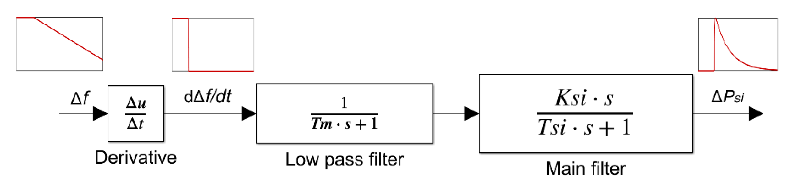
3.1. Derivation of the Method

The SI concept is derived assuming that the frequency dependence of loads is negligible and that in the timeframe of interest, i.e., soon after the disturbance, the frequency response is limited only by the system inertia. A power change ΔP in this system will cause a change in the rotational speed of rotating masses Δω according to the following relationship in its linearised form:
Δ ω ( t )   =   1 2 H s y s ( Δ P ) d t
Taking the integral of power imbalance over time and considering Equation (3), one obtains:
Δ f ( t ) =   f n 2 H s y s S s y s Δ P · t = RoCoF · t
Thus, in order to limit RoCoF over certain period of time, power imbalance ΔP has to be limited. It is, however, difficult because the magnitude of power imbalance is often unknown at the time of its occurrence. Instead, what can be anticipated is the maximum power of a power infeed or load that is in operation, and for this loss, the system can be adjusted. Applying Equation (3) to the worst-case tripping of power supply maximum RoCoF is obtained:
RoCoF max =   f n 2 H s y s S s y s Δ P max
Decreasing RoCoFmax to the required value, RoCoFlim, entails delivering power corresponding to the difference between the two RoCoF values,
RoCoF diff =   RoCoF max RoCoF lim
RoCoF diff =   f n 2 H s y s S s y s ( Δ P max Δ P lim ) = f n 2 H s y s S s y s Δ P diff
where Δ P diff is the power missing in the power system to reach the required RoCoF after the trip.
RoCoFlim is the system security setting as explained in Section 1 of this paper, here assumed to be ±1 Hz/s. RoCoFmax is the worst-case scenario RoCoF calculated in the operation planning phase. Equation (8), therefore, provides a description of how much power on average needs to be delivered in order to reach the required RoCoF. The proposed SI method answers the question how to do it and is explained below.
As described in [32], there has to be a clear distinction between global variations of system frequency and local faster oscillations caused by local imbalances. A measurement window of 500 ms is applied to neglect the latter. The integral of power (Equation (4)) is the energy surplus or deficit that is added or missing in the power system due to tripping of load or generation, respectively. Thus,
Δ f ( t ) =   f n 2 H s y s S s y s Δ E ( t )  
Now, assuming that Δ f ( t ) at t = 500 ms after the trip cannot be larger than that resulting from RoCoFlim, a formula expressing the amount of energy Δ E 1s needed to be supplied in time t in order to change RoCoF by RoCoFdiff is obtained:
Δ E 500 ms =   2 H s y s S s y s f n RoCoF diff  
Proposed controller structure to deliver ΔE500ms is presented in Figure 2. The main premise is that the controller will act only in a short timeframe, which corresponds to the inertial response of the system. In this case, according to Equation (5), the input signal to this controller will be in a form of a linear decrease (or rise, depending on power imbalance sign); therefore, in order to transform it to a constant signal, a derivative function is used. Then, a stabilising low-pass filter and main filter are used to shape the response of the synthetic inertia to a step change in a desired manner.
For the proposed transfer function,
G S I ( s ) = K S I · s ( T m s + 1 ) ( T S I s + 1 )  
The unit step response is given by,
y S I ( t ) = P S I ( t ) = K S I T m T S I ( e t T m e t T S I )  
Taking a definite integral of Equation (12) over a specified time, τ, yields the amount of energy supplied by the device offering the SI service,
Δ E τ   = 0 τ P S I ( t ) d t = K S I T S I T m T S I ( e τ T S I 1 ) K S I T m T m T S I ( e τ T m 1 )
Thus, by tuning gain and time constants of GSI(s) the main control objective can be met:
Δ E τ Δ E 500 m s  

3.2. Tuning of Synthetic Inertia Controller

Tuning of the main filter can be performed under the following considerations. In the abovementioned derivation, it was assumed that RoCoF is measured and additional energy should be supplied within time τ. In general, this period can be arbitrary but should be related to the characteristics of the expected frequency response of the system, in particular to time of occurrence of frequency nadir. Figure 3a shows a comparison of typical governors reacting to a sudden load change causing frequency decrease. Total system inertia Hsys = 4 s was assumed in this case. The grey area corresponds to primary frequency control response range, which should deploy its full reserves within several to fifteen seconds. However, for considerable load imbalances this reaction might be too slow, and the frequency might drop to a level where under-frequency protection might be triggered, thus additional support has to be introduced in order to retain RoCoF above the required level. This support can be offered by synthetic inertia in a much faster regime, during the inertial response period marked as the red area.
Consequently, TSI should be selected in such a way that most of the time response of GSI(s) passes before time τ, as depicted in Figure 3b. This guarantees that the inertial response will not overlap with the FFR response too much. Calculation of the main gain KSI is possible based on Equations (10) and (13). It should be noted, however, that the proposed controller is an open-loop controller, and by definition, its output depends on the magnitude of the input. The magnitude of the input, which is Δf, initially depends on the size of the disturbance but shortly after is influenced by instantaneous power delivered by the SI (which is the controller’s output). Thus, the required energy E500ms can be delivered only if RoCoF is equal to RoCoFlim, which can happen only if Eτ is equal to E500ms. In practice, it is impossible to keep this equilibrium during the dynamic process, thus small deviations should be expected.

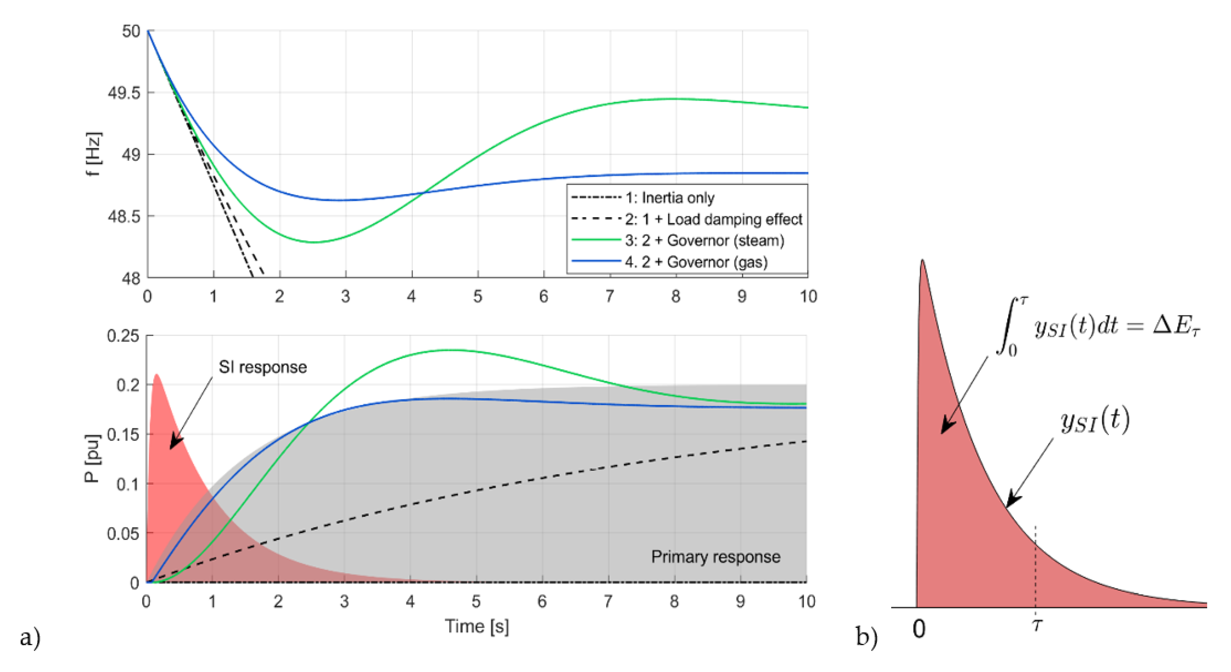
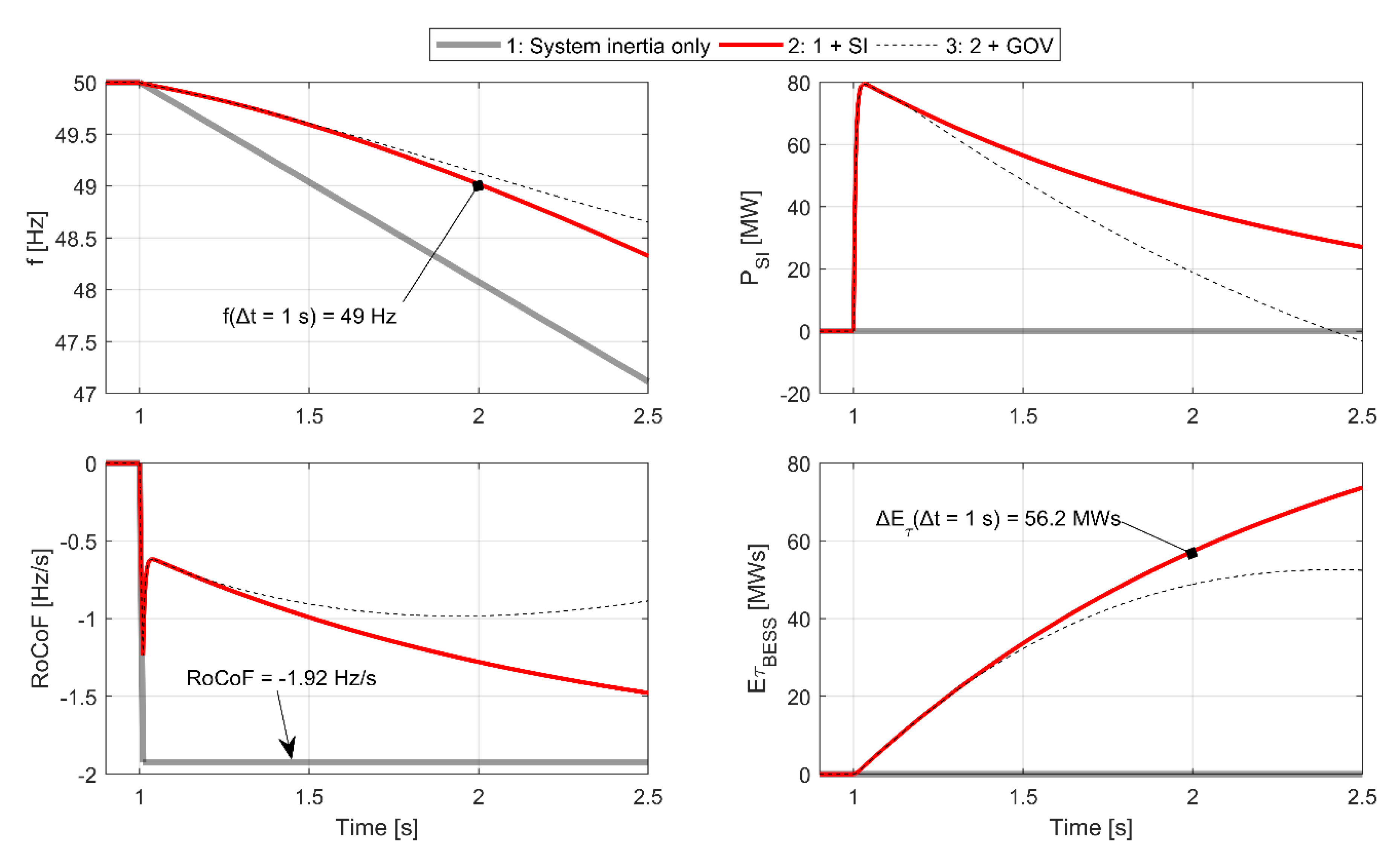
3.3. Synthetic Inertia Concept Verification Based on Simple Theoretical Model of a Power System

A modified version of the IEEE 14-bus system shown in Figure 4 is used for the purpose of providing a proof of concept. The modification regarded ratings of the machines and their type are presented in Table 1. The example is based on data from Scenario 2, in which the largest generation trip was 117 MW (G3). Data for this power flow are provided in Table 1, whereas the calculations are confirmed by the plots in Figure 5. Based on Equation (6), the resulting RoCoFmax for this ΔP is equal to 1.92 Hz/s, whereas the goal is to limit the RoCoF to RoCoFlim = 1.0 Hz/s. According to Equation (10), this task entails delivering additional energy E1s from BESS equal to 56.2 MWs within the time of contribution of synthetic inertia, which in this case, is assumed to be one second. As a rule of thumb, the controller measurement time constant, Tm, is selected to be equal to 20 ms. An inherent feature of the controller described by Equation (12) with Tm = 0.02 s is that after time τ = TSI, it will deliver 61% of total energy, and after time τ = 2 TSI, 86% of energy, which is a direct consequence of Equation (13). By using this relationship, the main time constant TSI can be adjusted to satisfy the requirement of the speed of response of the SI controller. Finally, based on Equations (13) and (14), gain KSI can be calculated to match the required amount of energy Δ E τ and, in this example, is equal to 61.49 MWs/Hz.
Figure 5 shows the result of G3 outage for three configurations of frequency control in the power system. The theoretical case with only inertial response is shown in red; the case with added SI contribution tuned according to the rules described above is shown in thick grey, whereas the same case with primary frequency control active is marked with a dashed line. Synthetic inertia brings considerable improvement to the frequency decline process: the frequency does not drop under the assumed level of 49.0 Hz during the first second, indicating that the average RoCoF is not lower than −1 Hz/s. The results also confirm that for the time period of interest, i.e., up to 1 s after the disturbance, the frequency response can be considered linear, which is the main assumption for parameterisation of the controller. The last plot in Figure 5 shows energy delivered to the power system by BESS during this disturbance. One second after the outage, it reached the value of 56.2, which fulfils the control objective expressed by Equation (14).

4. System Operation Planning Methodology with Focus on RoCoF

As explained in Section 1, the assessment of inertia adequacy to support the required RoCoF throughout the whole planning period can be based on Equation (1) only if synchronous generators are the only type of generation supplying the system with power. Then, it is a matter of summing their respective kinetic energy and identifying the largest possible trip in the power system. However, this simple methodology does not enable us to include other inertia-providing resources in the calculation. For instance, virtual inertia provided by wind turbines or synthetic inertia from BESS with different energy to power ratios and control principles would be very difficult to be accurately represented in this equation. Therefore, there is a need for frequency stability assessment methodology that takes into account non-synchronous contributors to system inertia and frequency support. This methodology is explained below. It consists of five steps depicted in Figure 6.
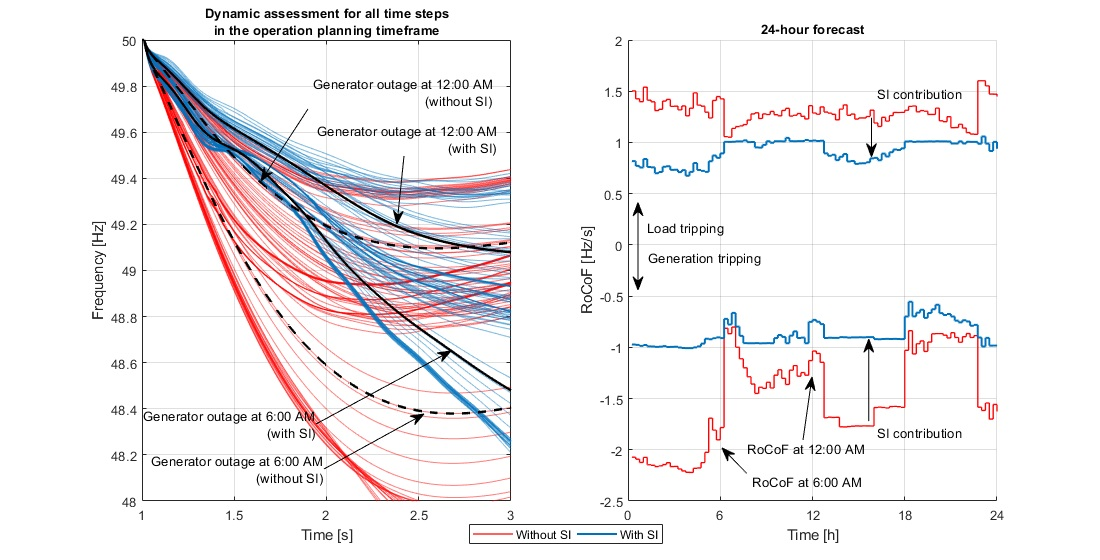
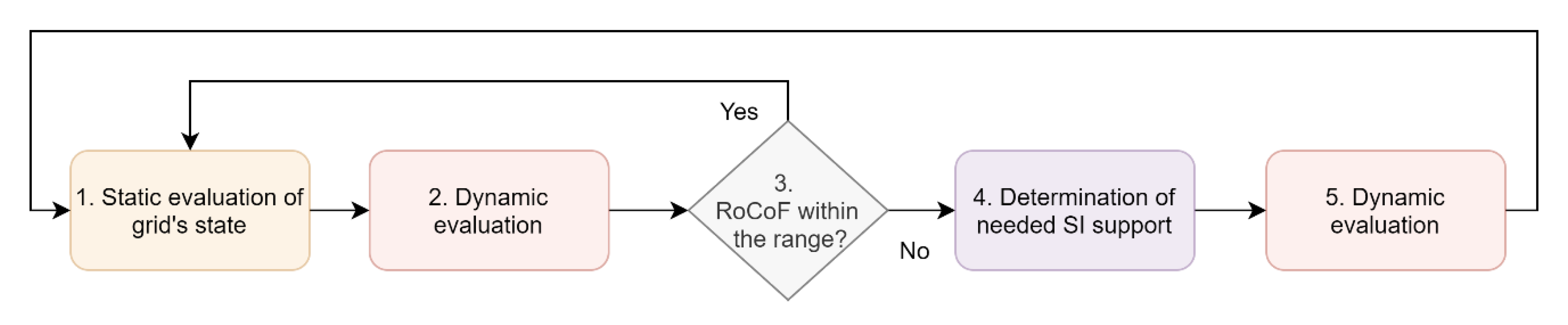
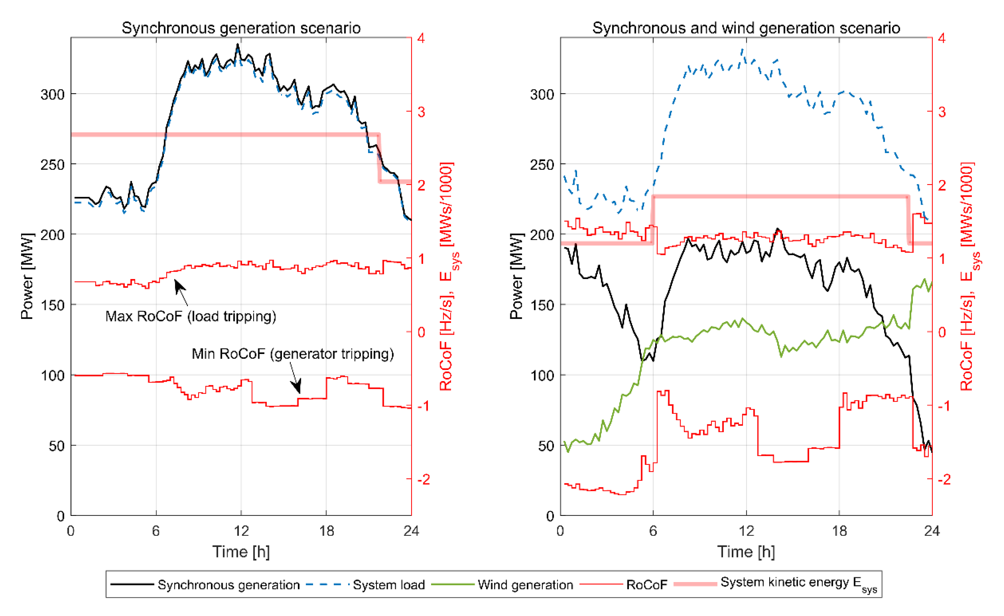
  • For each time step of the forecast the algorithm starts with static evaluation of the grid’s state through a load flow. In this stage equivalent, system inertia is calculated according to Equation (2), and based on Equation (3), maximum and minimum RoCoF are calculated for load and generation tripping, respectively. ΔP in this equation is the largest possible active power imbalance found in the load flow data.
  • In the second stage, dynamic evaluation is performed. This step might be considered optional for Scenario 1 but is a must for Scenario 2, if wind generation or other devices operating in the power system are equipped with synthetic inertia. The purpose is to accurately determine RoCoF through dynamic simulation of a power system model that encompasses dynamic responses of relevant elements to frequency changes.
  • Step three is a simple check—if the resulting value of RoCoF is within the predefined range, the algorithm moves to another time step, as the system is able to withstand the largest possible outage in given grid operation conditions. If not, Step 4 is executed.
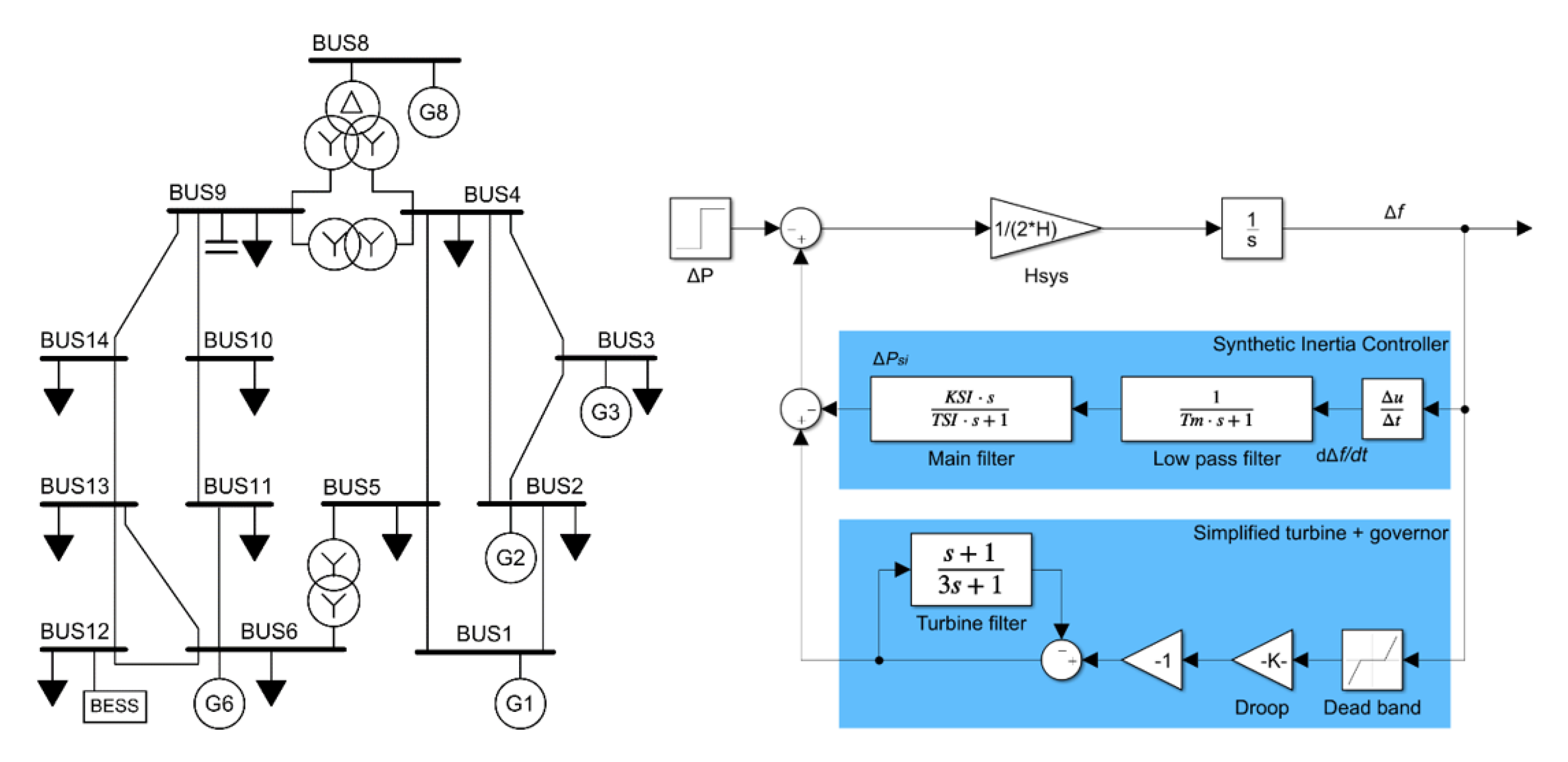
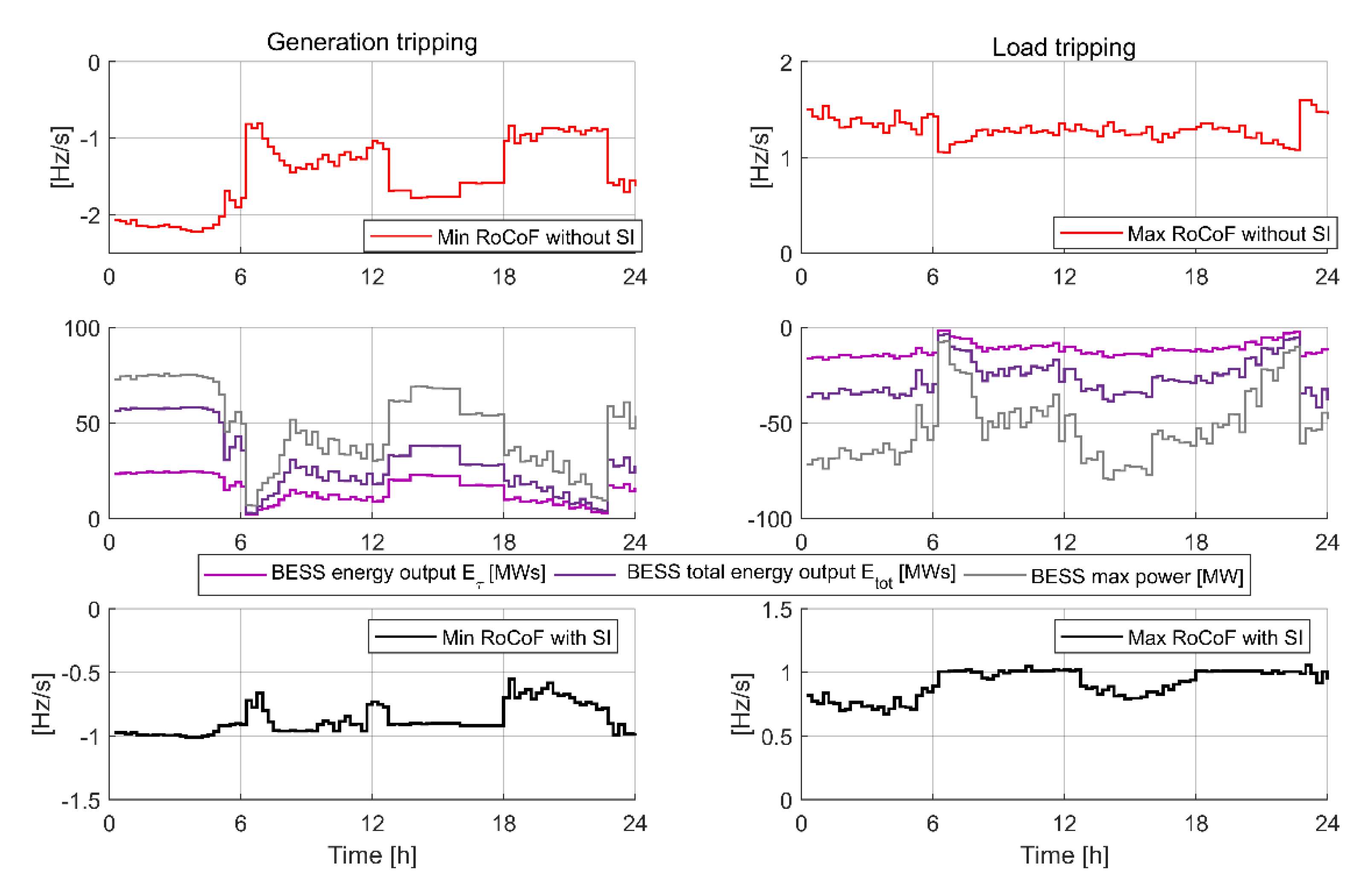
  • Step four consists in determining necessary additional inertia to keep RoCoF in the assumed range, i.e., between RoCoFmin for generation trip and RoCoFmax for load trip. The methodology is demonstrated using BESS, which are used for SI service due to their excellent controllability but support from other devices is also possible. Then, based on Equations (10) and (13), controller parameters are calculated. In fact, controller’s time constants do not have to be updated often. They could even be hardcoded in the SI controllers based on average inertia level in the power system and response time of fast frequency control of the frequency-governing devices. On the other hand, the overall SI gain needs to be calculated for every time step, as it influences the contribution level of SI.
  • In Step five, the SI is distributed among selected assets by assigning a weighting factor to each device so that the sum of weighting factors is equal to 1, and final dynamic simulation is performed to confirm the calculations. It has to be noted that more than one BESS or other device can take part in SI service. Calculated energy ΔEτ can be distributed among available units arbitrarily by the TSO, e.g., by engaging units being furthest from their respective limits, or by typical market mechanisms, such as merit order or long-term contracts, etc.
In the presented case, time series data for 24 h period in 15 min interval is available. These data represent forecasted system load and generation. The results of a set of load flow calculations are presented in Figure 7. Left-hand side plot shows a scenario in which only synchronous generation is present. The plot shows generation (black line) and system load (blue dashed line) patterns and calculated system kinetic energy Esys (red thick line). Note the reduced value of Esys at night indicating temporary tripping of generators due to low demand night period. Expected worst-case scenario RoCoF can also be noticed (red line) and should it exceed the threshold level necessary actions could be taken, as described in Step 4. Right-hand side plot of Figure 7 is constructed for a scenario in which a part of synchronous generation is superseded by wind generation, whose total power output is marked with green line. Calculated system inertia is, thus, lower and resulting RoCoF is lower. In this scenario, generation is also switched off during the night because of wind generation supplying low system demand. Note that there are many intervals for which RoCoF is below the threshold of −1 Hz/s, thus synthetic inertia is introduced.
For each time interval a necessary amount of energy, ΔE500ms, is calculated, and the gain of the SI controller is changed accordingly, based on Equation (13). Figure 8 shows the result of SI activation in BESS for the scenario with synchronous and wind generation for the operation planning period depicted in Figure 7. RoCoF values for the system operating without SI are presented in the top row. Plots in the middle row show quantities associated with BESS and SI: maximum power reached during the transient (grey curve), energy output in the first 500 ms (ΔEτ, light purple curve) and total energy output during the transient (dark purple curve). The bottom plots show minimum and maximum RoCoF values for the scenario with SI active. None of the cases with RoCoF below −1 Hz/s or above 1 Hz/s are observed, which implies that the proposed synthetic inertia controller and deployment methodology can be an effective tool to address issues associated with too low inertia.
The dynamics of the frequency transients are depicted in Figure 9 for four distinct hours, corresponding to different system operating conditions. The same SI control parameters are used in all simulations except for the general gain, KSI, which is changed to achieve the required level of SI. Plots in the top row show power contribution from SI delivered by BESS. Since it is a multimachine system, the responses are more oscillatory than in the theoretical case shown in Figure 3, but the general characteristics of the inertial response are preserved. Note that after the rapid injection of active power has decayed the sign of active power changes to negative, as it is indirectly dependent on the second derivative of frequency (see Figure 2 for control block diagram). This issue is further explained in the subsequent section. Nevertheless, the SI controller improves the frequency decline phase of the frequency regulation process by increasing RoCoF to a permissible level.

5. Validation of the Synthetic Inertia Concept in Real-Time Simulation Environment

5.1. Real-Time Simulation Environment

The essential element of the proposed methodology for power system operation planning with focus on maintaining proper level of inertia and RoCoF is the synthetic inertia controller. As evident from Figure 2, the controller utilizes two derivative functions in the main control loop, thus it might be prone to abrupt changes in the measured input signal. Therefore, validation of its operation in a more accurate simulation environment than basic transient simulation program is necessary to evaluate dynamic limitations of the controller. What is more, a detailed model of battery should be available to account for any limitations possibly imposed by the dynamics of the charging and discharging process. Lastly, the frequency measurement process itself is a challenge if high accuracy and speed of response are required. All these conditions are met by RTDS.
IEEE 14-bus power system model based on [34] has been adopted for the purpose of RTDS testing [35,36]. The single line diagram of the test power system with BESS is the same as the one presented in Figure 4.

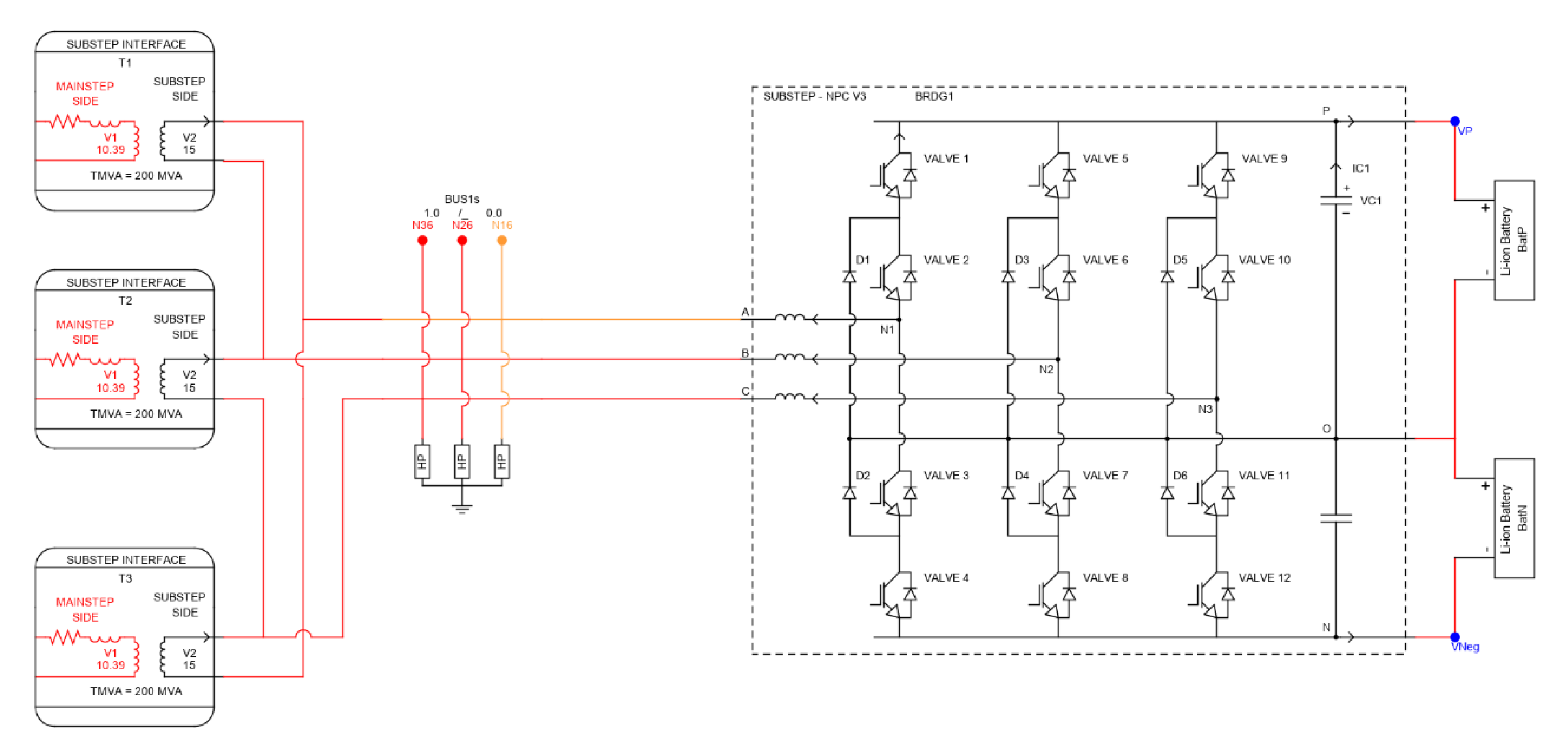
5.2. Battery Energy Storage System Model

BESS model simulated in RSCAD consists of two 9.69 MWh Li-ion batteries interfaced to the grid through three-phase three-level neutral point clamped (NPC) converter and a 10.4 V/15 kV transformer as shown in Figure 10. The converter operates at a switching frequency of 1250 Hz. BESS operates in power range of −100 MW÷100 MW. BESS model is determined by main parameters: number of cells in a stack (10,000), number of stacks in parallel (300) and capacity of a single cell (0.85 Ah).
The battery is represented by the “Min/Rincon-Mora” model [37]. It was extracted from a real commercial Li-ion polymer battery, TCL-PL-383562 from TCL Hyperpower Batteries Inc. The modelling method is focused on the electrical behaviour of the battery and voltage-current characteristics and, as such, is considered to be adequate for this study in which high power gradients are expected.

5.3. Synthetic Inertia Controller in RTDS

BESS’s converter is controlled using dq decoupled control with PI controllers both for the inner loop of current control and outer loop of active and reactive power control. The SI controller is integrated with the main control loop by means of auxiliary active power order signal that is added to the main power reference of BESS. The input to the SI controller is system frequency measured by the by phase-locked loop (PLL). Internal transfer function of the controller is depicted in Figure 11. Apart from the elements also represented in Figure 2, the lower part of the diagram contains blocks that prevent BESS from consuming or delivering power when conventional inertia would, but which would entail slowing down frequency restoration process, i.e., when df/dt ≠ 0 and PSI > 0 when f < fn or PSI < 0 when f > fn.
A comparison of frequency response of the system without synthetic inertia support, with basic controller and with the improved controller, is depicted in Figure 12. The simulated disturbance is a sudden loss of 40 MW produced by a wind farm. This causes a drop in frequency with RoCoF (measured with 100 ms averaging) reaching −1.6 Hz/s and nadir at the level of 48.6 Hz for the variant without SI support. When the support is added without the extra blocking logic, RoCoF is shifted to about −0.85 Hz/s, but due to the fact that BESS is draining power when RoCoF is rising, the whole recovery process is prolonged, and nadir is even decreased. Blocking logic described above, although it introduces nonlinearity to the control structure, improves the response of synthetic inertia by improving RoCoF without lengthening the whole process.
The whole control process in SI controller depends on a reliable frequency measurement. Frequency measurements can often be problematic when voltage asymmetry or distortion is encountered. Here, a standard PLL is used, as it offers stable and filtered measurement with tuneable dynamic performance. Operation of the PLL and its influence on the overall control process is analysed below.
PLL performance is examined for a three-phase and single-phase short-circuit in the grid. As can be deduced from Figure 13, PLL with typical settings appropriate for power electronic applications, here referred to as “Fast PLL”, produces large overshoot for the three-phase short-circuit and highly oscillatory response for the single-phase disturbance. However, when the PLL is purposely detuned to be much slower, both the overshoot and oscillations are much lower (compare blue and black signal PSI ref). The last row of plots shows that irrespective of PLL settings, the power converter of BESS is unable to deliver active power requested by SI due to too high-voltage distortion. This is however, out of scope of this paper. Nevertheless, application of the slower PLL is sufficient for frequency measuring purpose.

6. Conclusions

Control concept based on double derivative proved to be an appropriate solution for a synthetic inertia controller due to its inherent features, mainly self-decaying response, and straightforward scalability. Stability of control, on the other hand, results from open-loop structure and robust frequency measurement method offered by the PLL. Such a control structure is suitable for the purpose of RoCoF limitation, which is the main goal of the proposed operation planning methodology for low inertia systems. This methodology, by combining power-flow calculations and dynamic simulation, can be a helpful tool for the system operation planner or system dispatcher to determine possible issues with frequency stability related to too low inertia and, should this happen, schedule countermeasures such as the synthetic inertia proposed in this paper.

Author Contributions

Conceptualization, M.K.; methodology, M.K. and A.W.; software, A.W.; validation, M.K., A.W. and R.R.; formal analysis, A.W. and R.C.; investigation, A.W. and M.K.; resources, A.W., R.C., R.R. and C.N.P.; data curation, V.E. and G.G.; writing—original draft preparation, A.W., M.K. and R.R.; writing—review and editing, R.C. and C.N.P.; visualization, M.K.; supervision, M.D.S. and V.E.; project administration, M.D.S.; funding acquisition, M.D.S., V.E. and G.G. All authors have read and agreed to the published version of the manuscript.

Funding

This research was funded by European Union’s Horizon 2020 Research and Innovation Programme grant number 773708.

Institutional Review Board Statement

Not applicable.

Informed Consent Statement

Not applicable.

Acknowledgments

The project INTERPLAN has received funding from the European Union’s Horizon 2020 Research and Innovation Programme under Grant Agreement No. 773708.

Conflicts of Interest

The authors declare no conflict of interest.

References

  1. ENTSO-E. Ten Year Network Development Plan (TYNDYP); 2020 Scenario Report; ENTSO-E: Brussels, Belgium, 2020. [Google Scholar]
  2. ENTSO-E; Technical Group on High Penetration of Power Electronic Interfaced Power Sources. High Penetration of Power Electronic Interfaced Power Sources and the Potential Contribution of Grid Forming Converters; Technical Report; ENTSO-E: Brussels, Belgium, 2020. [Google Scholar]
  3. Austalian Energy Market Operator. Black System, South Australia, 28 September 2016—Final Report; Australian Energy Market Operator: Melbourne, Australia, 2017. [Google Scholar]
  4. O’Conell, B.; Cunniffe, N.; Eager, M.; Cashman, D.; O’Sullivan, J. Assessment of Technologies to Limit the Rate of Change of Grid Frequency on an Island System; CIGRE: Paris, France, 2018. [Google Scholar]
  5. ENTSO-E. European Power System 2040: Completing the Map. System Needs Analysis, Part of ENTSO-E’s 2025, 2030, 2040 Network Development Plan 2018; ENTSO-E: Brussels, Belgium, 2019. [Google Scholar]
  6. ENTSO-E. High Penetration of Power Electronic Interfaced Power Sources (HPoPEIPS) ENTSO-E Guidance Document for National Implementation for Network Codes on Grid Connection; ENTSO-E: Brussels, Belgium, 2017. [Google Scholar]
  7. Machowski, J.; Lubośny, Z. Stabilność Systemu Elektroenergetycznego; Wydawnictwo Naukowe PWN: Warsaw, Poland, 2018; ISBN 978-83-01-20006-0. [Google Scholar]
  8. ENTSO-E. Need for Synthetic Inertia (SI) for Frequency Regulation: ENTSO-E Guidance Document for National Implementation for Network Codes on Grid Connection; ENTSO-E: Brussels, Belgium, 2018. [Google Scholar]
  9. European Commission. Commission Regulation (EU) 2016/631 of 14 April 2016 Establishing a Network Code on Requirements for Grid Connection of Generators (Text with EEA Relevance); European Commission: Brussels, Belgium, 2016. [Google Scholar]
  10. European Commission. Commission Regulation (EU) 2016/1447 of 26 August 2016 Establishing a Network Code on Requirements for Grid Connection of High Voltage Direct Current Systems and Direct Current-Connected Power Park Modules (Text with EEA Relevance); European Commission: Brussels, Belgium, 2016. [Google Scholar]
  11. European Commission. Commission Regulation (EU) 2016/1388 of 17 August 2016 Establishing a Network Code on Demand Connection; European Commission: Brussels, Belgium, 2016. [Google Scholar]
  12. ENTSO-E. Rate of Change of Frequency (RoCoF) Withstand Capability ENTSO-E Guidance Document for National Implementation for Network Codes on Grid Connection; ENTSO-E: Brussels, Belgium, 2018. [Google Scholar]
  13. National Grid ESO. Operability Strategy Report; National Grid ESO: Warwick, UK, 2019. [Google Scholar]
  14. Energy Networks Association. The Accelerated Loss of Mains Change Programme: Stakeholder Event; National Grid ESO: Warwick, UK, 2019. [Google Scholar]
  15. You, S.; Liu, Y.; Tan, J.; Gonzalez, M.T.; Zhang, X.; Zhang, Y.; Liu, Y. Comparative Assessment of Tactics to Improve Primary Frequency Response Without Curtailing Solar Output in High Photovoltaic Interconnection Grids. IEEE Trans. Sustain. Energy 2019, 10, 718–728. [Google Scholar] [CrossRef]
  16. Sami, S.S.; Meng, C.; Jianzhong, W. Modelling and Control of Multi-Type Grid-Scale Energy Storage for Power System Frequency Response. In Proceedings of the 2016 IEEE 8th International Power Electronics and Motion Control Conference (IPEMC-ECCE Asia), Hefei, China, 22–25 May 2016; pp. 269–273. [Google Scholar]
  17. Knap, V.; Sinha, R.; Swierczynski, M.; Stroe, D.; Chaudhary, S. Grid Inertial Response with Lithium-Ion Battery Energy Storage Systems. In Proceedings of the 2014 IEEE 23rd International Symposium on Industrial Electronics (ISIE), Istanbul, Turkey, 1–4 June 2014; pp. 1817–1822. [Google Scholar]
  18. Eriksson, R.; Modig, N.; Elkington, K. Synthetic Inertia versus Fast Frequency Response: A Definition. IET Renew. Power Gener. 2017, 12. [Google Scholar] [CrossRef]
  19. Gao, Q.; Preece, R. Improving Frequency Stability in Low Inertia Power Systems Using Synthetic Inertia from Wind Turbines. In Proceedings of the 2017 IEEE Manchester PowerTech; IEEE: Manchester, UK, June 2017; pp. 1–6. [Google Scholar]
  20. Gonzalez-Longatt, F.M. Effects of the Synthetic Inertia from Wind Power on the Total System Inertia: Simulation Study; IEEE: Manchester, UK, 2012; p. 8. [Google Scholar]
  21. Gevorgian, V.; Koralewicz, P.J.; Villegas Pico, H.N.; Shah, S.D.; Wallen, R.B.; Corbus, D.A.; Keller, J.A.; Hovsapian, R.; Mohanpurkar, M.; Kadavi, R.; et al. WGRID-49 GMLC Project Report: Understanding the Role of Short-Term Energy Storage and Large Motor Loads for Active Power Controls by Wind Power; OSTI: Oak Ridge, TN, USA, 2019.
  22. Jiebei, Z.; Booth, C.D.; Adam, G.P.; Roscoe, A.J. Inertia Emulation Control of VSC-HVDC Transmission System. In Proceedings of the 2011 International Conference on Advanced Power System Automation and Protection; IEEE: Beijing, China, 2011; pp. 1–6. [Google Scholar]
  23. Debbarma, S.; Hazarika, C.; Singh, K.M. Virtual Inertia Emulation from HVDC Transmission Links to Support Frequency Regulation in Presence of Fast Acting Reserve. In Proceedings of the 2018 2nd International Conference on Power, Energy and Environment: Towards Smart Technology (ICEPE), Meghalaya, India, 1–2 June 2018; pp. 1–6. [Google Scholar]
  24. Haileselassie, T.M.; Uhlen, K. Primary Frequency Control of Remote Grids Connected by Multi-Terminal HVDC. In Proceedings of the IEEE PES General Meeting; IEEE: Minneapolis, MN, USA, 2010; pp. 1–6. [Google Scholar]
  25. Gonzalez-Longatt, F.M. Activation Schemes of Synthetic Inertia Controller on Full Converter Wind Turbine (Type 4). In Proceedings of the 2015 IEEE Power & Energy Society General Meeting; IEEE: Denver, CO, USA, 2015; pp. 1–5. [Google Scholar]
  26. Chamorro, H.R.; Riaño, I.; Gerndt, R.; Zelinka, I.; Gonzalez-Longatt, F.; Sood, V.K. Synthetic Inertia Control Based on Fuzzy Adaptive Differential Evolution. Int. J. Electr. Power Energy Syst. 2019, 105, 803–813. [Google Scholar] [CrossRef] [Green Version]
  27. Chamorro, H.R.; Malik, N.R.; Gonzalez-Longatt, F.; Sood, V.K. Evaluation of the Synthetic Inertia Control Using Active Damping Method. In Proceedings of the 2017 6th International Conference on Clean Electrical Power (ICCEP); IEEE: Santa Margherita Ligure, Italy, 2017; pp. 269–274. [Google Scholar]
  28. Chamorro, H.R.; Sanchez, A.C.; Overjordet, A.; Jimenez, F.; Gonzalez-Longatt, F.; Sood, V.K. Distributed Synthetic Inertia Control in Power Systems. In Proceedings of the 2017 International Conference on ENERGY and ENVIRONMENT (CIEM); IEEE: Bucharest, Hungary, 2017; pp. 74–78. [Google Scholar]
  29. Knap, V.; Chaudhary, S.K.; Stroe, D.; Swierczynski, M.; Craciun, B.; Teodorescu, R. Sizing of an Energy Storage System for Grid Inertial Response and Primary Frequency Reserve. IEEE Trans. Power Syst. 2016, 31, 3447–3456. [Google Scholar] [CrossRef] [Green Version]
  30. Kundur, P.; Balu, N.J.; Lauby, M.G. Power System Stability and Control; McGraw-Hill: New York, NY, USA, 1994; Volume 7. [Google Scholar]
  31. Stenclik, D.; Richwine, M.; Miller, N.; Hong, L. The Role of Fast Frequency Response in Low Inertia Power Systems; CIGRE: Paris, France, 2018. [Google Scholar]
  32. EIRGRID. System Operator for Northern Ireland. RoCoF Modification Proposal—TSOs’ Recommendations; EIRGRID: Dublin, Ireland, 2012. [Google Scholar]
  33. Pourbeik, P. Simple Model Specification for Battery Energy Storage System; EPRI: Washington, DC, USA, 2015. [Google Scholar]
  34. Freris, L.L.; Sasson, A.M. Investigation of the Load-Flow Problem. Proc. Inst. Electr. Eng. 1968, 115, 1459–1470. [Google Scholar] [CrossRef]
  35. Report, I.C. Excitation System Models for Power System Stability Studies. IEEE Trans. Power Appar. Syst. 1981, PAS-100, 494–509. [Google Scholar] [CrossRef]
  36. Report, I.C. Dynamic Models for Steam and Hydro Turbines in Power System Studies. IEEE Trans. Power Appar. Syst. 1973, PAS-92, 1904–1915. [Google Scholar] [CrossRef]
  37. Min, C.; Rincon-Mora, G.A. Accurate Electrical Battery Model Capable of Predicting Runtime and I-V Performance. IEEE Trans. Energy Convers. 2006, 21, 504–511. [Google Scholar] [CrossRef]
Figure 1. A. Frequency response stages as described in [29].
Energies 14 00737 g001
Figure 2. Proposed structure of the synthetic inertia controller and visualization of the idealized control signals (above).
Energies 14 00737 g002
Figure 3. (a) Response to generation trip (0.2 pu) of 1. purely inertial system (dash–dot line), 2. inertial system with power-frequency load characteristics, 3. as in 2 with simplified steam turbine with governor added, 4. as in 2 with simplified gas turbine with governor added; (b) shape of time response of GSI(s).
Energies 14 00737 g003
Figure 4. Single line diagram of the modified 14-bus IEEE system with BESS added to bus 12; the BESS model is a generic current injection model with WECC BESS Control System for RMS simulation [33] (left) and equivalent block diagram for this model in a lumped form (right).
Energies 14 00737 g004
Figure 5. Response to generation trip of 1. purely inertial system (grey line); 2. inertial system with synthetic inertia (SI support exhibiting linear decline of frequency in the first 0.5 s (red line); 3. same as no. 2 but with governor action (dashed line).
Energies 14 00737 g005
Figure 6. Methodology for frequency stability assessment and synthetic inertia provision.
Energies 14 00737 g006
Figure 7. Generation and consumption data (forecast) for the planning timeframe; plots represent data processed in Step 1 of the proposed methodology.
Energies 14 00737 g007
Figure 8. Effect of SI activation on rate of change of frequency (RoCoF) for the 24 h planning period for generation tripping (left) and load tripping (right): RoCoF for the scenario with synchronous and wind generation (top), BESS power and energy output (middle), RoCoF for the same scenario with SI activated.
Energies 14 00737 g008
Figure 9. Reponses to generation trip of the system equipped with SI (blue) and without SI (grey) for four different instants during the planning period.
Energies 14 00737 g009
Figure 10. The diagram of BESS with batteries, neutral point clamped (NPC) converter with firing controller, filter and transformer.
Energies 14 00737 g010
Figure 11. Synthetic inertia control diagram for BESS; the output of the controller can be either signal P_SI: normal operation of SI or blocked blocking criteria are met.
Energies 14 00737 g011
Figure 12. Comparison of responses to 40 MW trip: with no synthetic inertia support (blue), with SI support without blocking logic (black) and with SI with blocking logic (green).
Energies 14 00737 g012
Figure 13. Comparison of SI controller response to three-phase short-circuit (left column) and singe-phase short-circuit (right column) for fast (kp = 5, Ti = 0.01 s) and slow (kp = 1, Ti = 0.15 s) PLL settings.
Energies 14 00737 g013
Table 1. Operating point of generators in the modified 14-bus IEEE system.
Gen 1Gen 2Gen 3Gen 6Gen 8
TypeSynchronousSynchronousSynchronousWindWind
Rating [MVA]/Load [MW]200/50220/30160/11772/49100/77
H [s]3.24.02.000
Publisher’s Note: MDPI stays neutral with regard to jurisdictional claims in published maps and institutional affiliations.

