Radial Turbine Design for Solar Chimney Power Plants

Abstract

Solar chimney power plants (SCPPs) collect air heated over a large area on the ground and exhaust it through a turbine or turbines located near the base of a tall chimney to produce renewable electricity. SCPP design in practice is likely to be specific to the site and of variable size, both of which require a purpose-built turbine. If SCPP turbines cannot be mass produced, unlike wind turbines, for example, they should be as cheap as possible to manufacture as their design changes. It is argued that a radial inflow turbine with blades made from metal sheets, or similar material, is likely to achieve this objective. This turbine type has not previously been considered for SCPPs. This article presents the design of a radial turbine to be placed hypothetically at the bottom of the Manzanares SCPP, the only large prototype to be built. Three-dimensional computational fluid dynamics (CFD) simulations were used to assess the turbine’s performance when installed in the SCPP. Multiple reference frames with the renormalization group k-$\epsilon$ turbulence model, and a discrete ordinates non-gray radiation model were used in the CFD simulations. Three radial turbines were designed and simulated. The largest power output was 77.7 kW at a shaft speed of 15 rpm for a solar radiation of 850 W/m${}^2$ which exceeds by more than 40 kW the original axial turbine used in Manzanares. Further, the efficiency of this turbine matches the highest efficiency of competing turbine designs in the literature.

1. Introduction

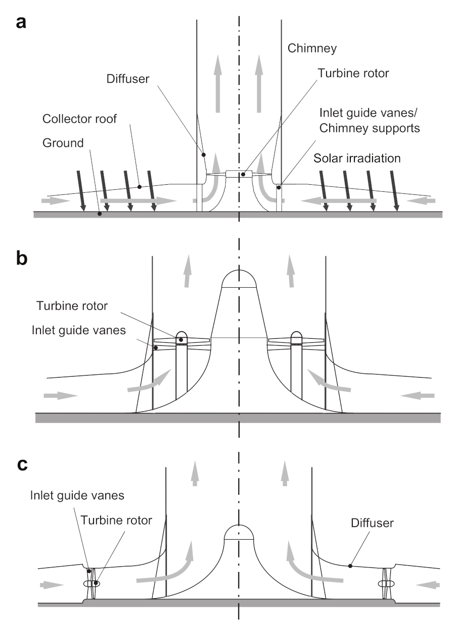
Solar chimney power plants (SCPPs) use solar radiation to increase the temperature of the air collected over a large area of ground, as shown in Figure 1. The resulting airflow drives one or more turbines shown at the base of the chimney. Only one large-scale SCPP demonstration prototype has been built, at Manzanares, Spain [1]. The mean collector radius was 122 m, the chimney height was 194.6 m, and the maximum output power was 37 kW. Due to its uniqueness, most of the literature on SCPP is based on analysis of, or comparisons to the Manzanares design.

The power conversion unit (PCU) comprises the turbine(s), power electronics, grid interface, and the flow passage from the collector exit to the chimney inlet [2]. The main component of the PCU studied in this paper is the turbine.

Previous SCPP prototypes have used axial turbines in different configurations. Gannon and Von Backström ([3,4]) designed and tested a turbine for a SCPP. A free vortex method was used to determine the main dimensions; then a matrix throughflow method (MTM) predicted the flow trough the inlet guide vanes (IGVs) and rotor; and finally, an optimization scheme coupled to a surface vortex method generated blades of minimum chord and low drag. The authors concluded that a total-to-total efficiency of 85–90% and a total-to-static efficiency of 77–80% could be expected in a full-scale turbine. From here on, this paper considers only the total-to-total efficiency. Von Backström and Gannon [5] presented an analytical method to find the influences of turbine flow, load coefficient, and degree of reaction on turbine efficiency for an SCPP. These characteristics were measured on a 720 mm diameter axial turbine model with 12 blades and 18 IGVs.

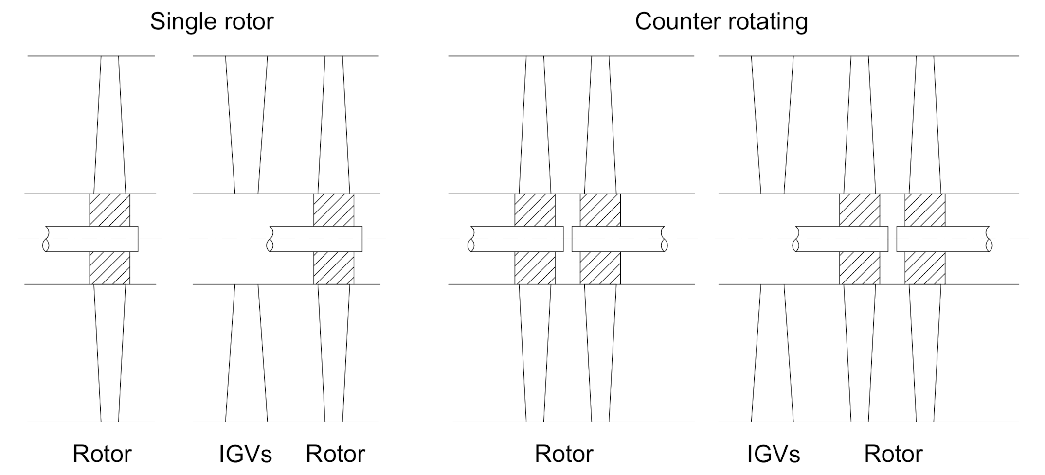
Denantes and Bilgen [7] compared three different turbine layouts using an efficiency model: single vertical axis (VA), six VA, and 36 horizontal axes (HA), as shown in Figure 2. Two different types of turbines are shown in Figure 3: a single runner turbine and a counter-rotating turbine with and without IGVs. The counter-rotating turbines had better performance at higher loads than the single runner turbines, but the latter showed better efficiency at solar radiation greater than 800 W/m${}^2$; SCPPs, however, work most of the time with solar radiation less than 800 W/m${}^2$. Another advantage for a counter-rotating turbine is that it can be designed without IGVs, which reduce the turbine efficiency.

Tingzhen et al. [8] numerically simulated a 3-bladed axial turbine for the Manzanares prototype, and a 5-bladed axial turbine for another 10 MW SCPP. The 3-bladed turbine had higher rotational speed than the 4-blade axial turbine installed in the Manzanares prototype for the same power output of 50 kW. Additionally, they found that a 2-bladed turbine could not extract the same power. They concluded that a 5-bladed turbine would have a maximum power output and efficiency of 10 MW and 50%, respectively. Fluri and Von Backström [2] analyzed the PCU in the three configurations of Figure 2. Configuration (a) generated the highest yearly energy yield; however, the peak torque was 474.3 MNm, making its drive train costly and its feasibility doubtful. The advantage of having more turbines is the distribution of the torque over the individual generators. Each of the six vertical axis turbines operated at a peak torque of 31.3 MNm, and each of the 32 horizontal axis turbines at 2.63 MNm. It is likely that multiple turbines would be more expensive than a single turbine for the same total power.

Rangel et al. [9] compared the VA and the HA turbines in [2,5] respectively to maximize the power in both configurations for the SCPP. CFD simulations showed that a VA turbine produced a maximum power of 78 kW at 58 rpm, and HA turbines produced 58 kW at 86 rpm. Zhou et al. [10] designed an axial turbine for a SCPP with vertical collector using the NACA 63-215 airfoil; they tested the performance of a scale model of the turbine in a wind tunnel where the maximum power was around 11 W at a wind speed of 8 m/s approximately. The conclusion was that the optimum number of blades was six, and the optimum tip speed ratio, defined as the ratio between the tangential speed of the tip of a blade and the actual speed of the wind, was 1.9.

Elmagid and Keppler [12] used the geometry of the chimney and collector of the Manzanares SCPP to design an axial turbine using free vortex analysis to find a first approximation of the blade shape. Then an MTM was used to calculate the airflow inflow and outflow angles; this method is able to simulate the radial inflow and axial outflow. A CFD simulation using ANSYS-CFX gave results in good agreement with the experimental data from [13].

Gholamalizadeh and Chung [14] compared three CFD models of an axial turbine in an SCPP. Two models used the standard k-$\epsilon$ turbulence model, and [15] used RNG k-$\epsilon$ with scalable wall functions and full buoyancy effects for the flow inside the SCPP. The authors claimed that the main reason for selecting the k-$\epsilon$ turbulence model is to reduce the mesh resolution at the wall because the computational cost for simulations is high. There are no previous turbulence studies for radial turbines in similar applications. Zhang et al. [16] used RNG k-$\epsilon$ in a mixed flow pump with guide vanes because it can accurately predict the flow separation, secondary flow, and vortex behavior in the wall region. It is a comparable study to the present one because both involve incompressible flow that changes direction, guide vanes, and curved blades.

Liu et al. [17] used wind turbine blade design methodology to increase the efficiency of axial turbines for SCPPs. Unfortunately, they chose a 1930s airfoil, the NACA 4418, when a more modern section may have led to higher efficiency. Blade element theory was applied to determine the blade airfoil chord and pitch.

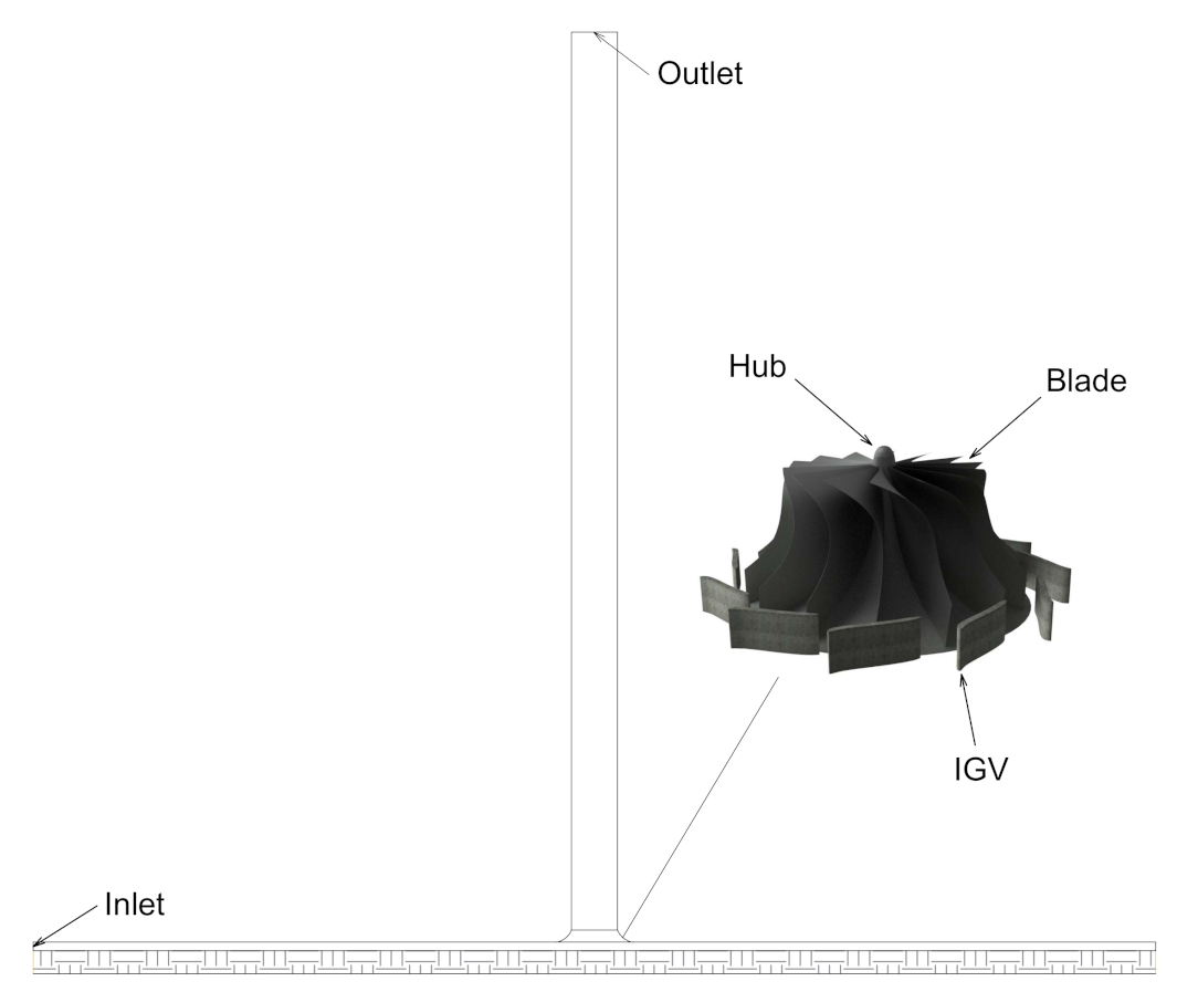
Caicedo [18] estimated the lifetime cost of electricity from SCPPs and summarized the findings in his Table 2.2. This shows the average cost of an SCPP turbine is 15% of the total SCPP investment, and is therefore significant. All the turbines described in this review require blade shapes that are specific to the SCPP being designed. Blades are normally made using molds so that changing the design requires making new molds. Molds, in turn, are expensive, so to improve the cost effectiveness of SCPPs, a turbine type that is new to this application and does not require expensive blade molds is proposed. This is the radial inflow (RIF) turbine shown conceptually in Figure 4. The blades have constant thickness and so can be rolled from a metal sheet or made using thin composite material. In addition, the blades would not require the high dimensional tolerance, as is necessary for efficient blades made from airfoil sections. As the turbine is located at the base of the chimney, the installation of the generator should be easier and cheaper than for some of the axial turbines shown above. The manufacturing and installation issues are not considered any further because the radial turbine can only be cost-effective if it has high efficiency. The paper concentrates, therefore, on using CFD with models for the turbulence, buoyancy effects, heat transfer, and solar radiation, to determine the performance of the turbine that is designed using a much simpler analysis. It is not feasible to use CFD for turbine design because of the large computational cost. The interested reader can find more general aspects of SCPP design in the extensive reviews by [10,19].

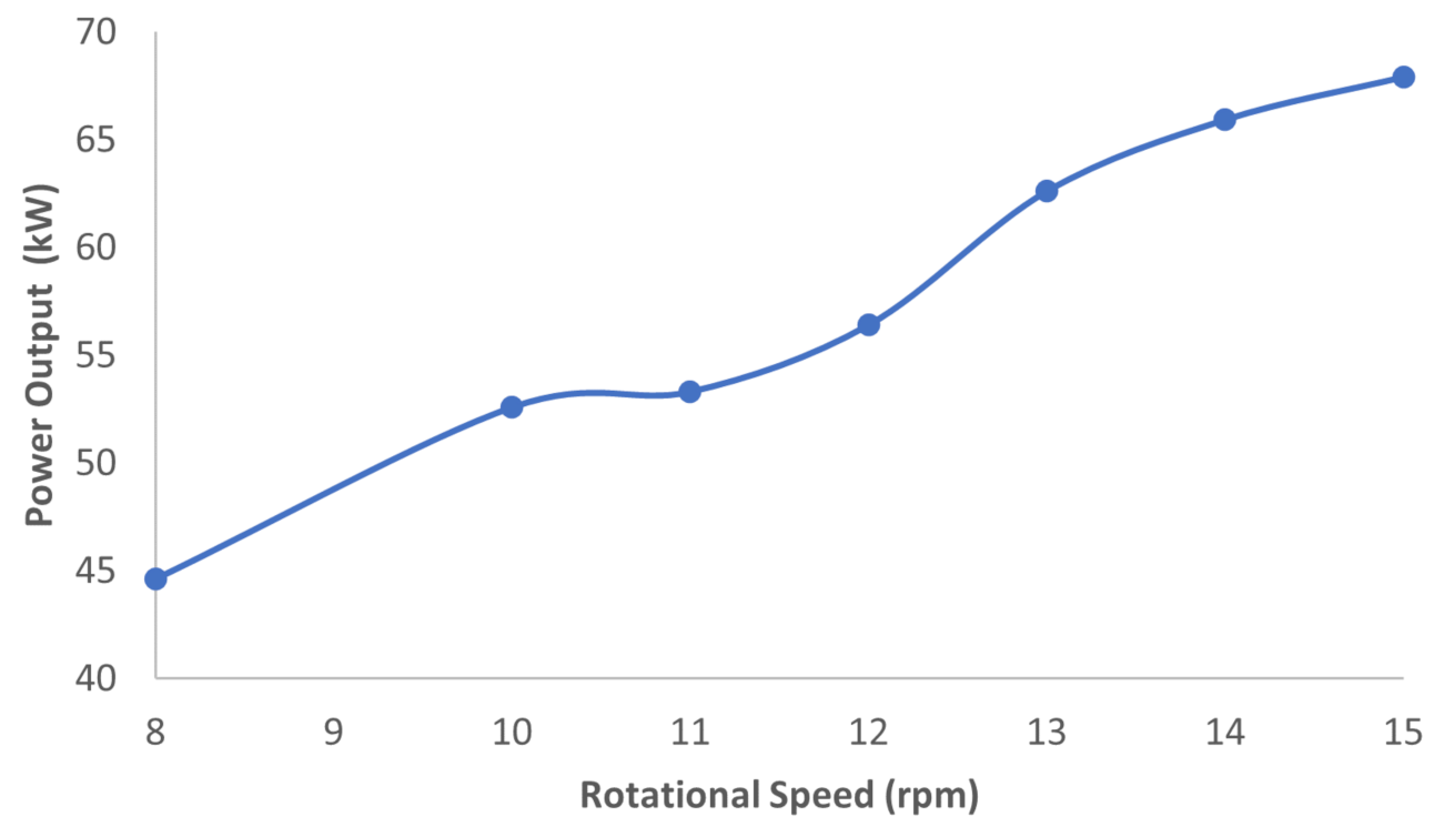
Previous designs considered axial turbines only. The main objective of this work was to assess the performances of several radial turbine designs for the Manzanares SCPP. CFD simulations were used to predict important parameters such as efficiency, power output, rotational speed, and torque. These performance parameters are compared to those of the axial flow turbine used at Manzanares and the axial turbines reviewed above. The feasibility of implementing custom-designed, low-cost radial turbines for SCPP applications in general is discussed.

The following section documents the governing equations that are applied to the whole system. Section 3 describes the turbine design, followed by a description of the CFD methodology. The results are presented in Section 5 and the conclusions in Section 6.

2. Governing Equations

The commercial CFD package ANSYS Fluent version 19.2 was used to solve the flow through the SCPP, including the rotating elements of the radial turbine. The steady, three-dimensional Navier–Stokes equations were solved with Reynolds-averaged Navier–Stokes (RANS) turbulence modeling closure. The next subsection describes the turbulence modeling used for the SCPP and for the turbine. The subsequent subsection describes the overall radiation and heat flow modeling, and the last covers the features specific to the turbine.

2.1. Collector and Chimney

The RANS equations are solved using the pressure-based coupled algorithm wherein the continuity and momentum equations are fully coupled. For brevity, these equations are not shown, and more detail is presented in [18]. The Boussinesq approximation is used because the density variations with temperature are small; the density is assumed constant in the convection terms, and in the gravitational term, it varies linearly with temperature [20]:

$$\rho ={\rho }_0\left(1-\beta \Delta T\right)$$

(1)

where $\beta$ is the thermal expansion coefficient.

The airflow in an SCPP is driven by natural convection. The effects of turbulence in natural convection flows depends on the relative magnitude of the buoyancy and viscous forces in the fluid, measured by the Rayleigh number ($Ra$). It is the product of the Grashof ($Gr$) and Prandtl ($Pr$) numbers:

$$Ra=\frac{g\beta \Delta T{L}^3\rho }{\mu \alpha }$$

(2)

where L is the mean collector height. Transition to turbulence occurs at $Ra$ > 10${}^9$ [21]. In the present case, $Ra$ > 10${}^{10}$ for the collector. Considering the experimental chimney velocity of 8.8 m/s at Manzanares taken from Figure 12b in [13], the Reynolds number at the chimney exit, $Re$ = $\rho$V_cD/$\mu$ > 5 × 10${}^6$, where V_c is the upwind velocity at the chimney and D is the diameter. $Re$ for the updraft tower in the present study is 7.4 × 10${}^6$. Based on the values of $Ra$ and $Re$, the flow is assumed to be turbulent.

RNG k-$\epsilon$ is the turbulence model selected for the whole domain. It has an improved performance compared to the standard k-$\epsilon$ model for swirling flows in which the geometry has a strong curvature [22]. The turbulent kinetic energy (k) and dissipation rate ($\epsilon$) are obtained from the following transport equations in inertial co-ordinates [23]:

$$\frac{\partial }{\partial x_i}\left(\rho k{u}_i\right)=\frac{\partial }{\partial x_j}\left({\alpha }_k{\mu }_{eff}\frac{\partial k}{\partial x_j}\right)+G_k+G_b-\rho \epsilon -Y_M$$

(3)

$$\frac{\partial }{\partial x_i}\left(\rho \epsilon u_i\right)=\frac{\partial }{\partial x_j}\left({\alpha }_k{\mu }_{eff}\frac{\partial \epsilon }{\partial x_j}\right)+C_{1\epsilon }\frac{\epsilon }{k}(G_k+C_{3\epsilon }{G}_b)-C_{2\epsilon }\rho \frac{{\epsilon }^2}{k}-R_{\epsilon }$$

(4)

where $G_k$, $G_b$, and $Y_M$ represent the generation of turbulence kinetic energy due to the mean velocity gradients, the generation of turbulence kinetic energy due to buoyancy, and the contribution of the fluctuating dilation in turbulence to the overall dissipation rate, respectively. $G_k$ and $G_b$ are used in this study. $C_{1\epsilon }$, $C_{3\epsilon }$, $C_{2\epsilon }$, and $R_{\epsilon }$ are other model constants whose values can be found in [23]. The accuracy of the RNG k-$\epsilon$ for the turbine was assessed by simulating a rotationally symmetric flow passage with one blade and no IGVs. The RNG k-$\epsilon$ and Menter’s shear stress transport (SST $k-\omega$) models are compared in Section 4.2.

2.2. Heat Transfer

The energy (E) equation [23] is solved in the following form:

$$\nabla ·\left[\overrightarrow{u_j}\left(\rho E+p\right)\right]=\nabla ·\left[k_{eff}\nabla T-\sum _j{h}_j\overrightarrow{J_j}+\left({\overline{\overline{\tau }}}_{eff}·\overrightarrow{u_j}\right)\right]+S_h$$

(5)

where $k\mathit{eff}$ is the effective conductivity (k + $k_t$, k is the fluid thermal conductivity and $k_t$ is the turbulent thermal conductivity); $\overrightarrow{Jj}$ is the diffusion flux of species j. S_h is the solar load.

The discrete ordinates (DO) radiation model solves the radiative transfer equation, for emission, absorption, and scattering, for a finite number of discrete solid angles, each associated with a vector direction $\overrightarrow{s}$ fixed in the global Cartesian system (x,y,z). It is possible to model semi-transparent walls, for example, the glass in the collector, and to model non-gray radiation using a gray-band model. The DO model equation is written as

$$\nabla ·\left[I_{\lambda }\left(\overrightarrow{r},\overrightarrow{s}\right)\overrightarrow{s}\right]+\left(a_{\lambda }+{\sigma }_s\right)I_{\lambda }\left(\overrightarrow{r},\overrightarrow{s}\right)=a_{\lambda }{n}^2{I}_{b\lambda }+\frac{{\sigma }_s}{4\pi }{\int }_0^{4\pi }{I}_{\lambda }\left(\overrightarrow{r},\overrightarrow{s}\right)\phi \left(\overrightarrow{s}·{\overrightarrow{s}}^{\prime }\right)d{\Omega }^{\prime }$$

(6)

where $\lambda$ is the wavelength, a_$\lambda$ is the spectral absorption coefficient, σ_s is the scattering coefficient, and I_$b\lambda$ is the black body intensity given by the Planck function [23]. Equation (6) can be integrated for each wavelength band, $\Delta \lambda$, by applying the non-gray DO model, resulting in transport equations for Iλ$\Delta \lambda$, the radiant energy contained in the wavelength band $\Delta \lambda$. The behavior in each band is assumed gray. The black body emission in the wavelength band per unit solid angle is written as

$$\left[F\left(0\to n{\lambda }_{2}T\right)-F\left(0\to n{\lambda }_{1}T\right)\right]n^2\frac{\sigma T_4}{\pi }$$

(7)

where F(0 →nλT) is the fraction of radiant energy emitted by a black body in the wavelength interval from 0 to $\lambda$ at temperature T in a medium of refractive index n. $\lambda$₂ and $\lambda$₁ are the wavelength boundaries of the band. The total intensity I_$\lambda$($\overrightarrow{r}$,$\overrightarrow{s}$) in each direction $\overrightarrow{s}$ at position $\overrightarrow{r}$ is computed using

$$I\left(\overrightarrow{r},\overrightarrow{s}\right)=\sum _k{I}_{\lambda k}\left(\overrightarrow{r},\overrightarrow{s}\right)\Delta {\lambda }_k$$

(8)

where the summation is over all the wavelength bands considered.

A solar model provided by ANSYS Fluent is used to calculate radiation that enters the computational domain [23]. There are two available options: solar ray tracing and DO irradiation. The solar ray tracing is used because it can be used for two bands, whereas the DO irradiation is restricted to one band. It applies the solar loads as heat sources (S_h). This solar model takes a beam that is modeled using the sun position vector and illumination parameters. These parameters are the direct and diffuse solar irradiation, and the spectral fraction of the visible part of the spectrum to the whole spectrum. The shading algorithm uses vector geometry where an opaque face completely shades the opposite face and a semi-transparent face attenuates the incident energy. All walls and inlet/outlet zones participate in the radiation heat transfer. It is available in the 3D solver only, and can be used in modeling steady and unsteady flows. The important wavelengths in solar energy are in the range of ultraviolet to near-infrared range, that is, from 0.29 to 25 μm. The radiation outside the atmosphere has the most energy; its wavelength range is from 0.25 to 3 μm. The radiation that reaches the ground is largely in the range from 0.29 to 2.5 μm [24]. This study considers two parts of the spectrum, the visible range (0.38 < $\lambda$ < 0.78 μm) and the infrared (0.78 < $\lambda$ < 2.5 μm). The fraction of incident solar radiation in the visible range out of the infrared range is 0.53.

2.3. Multiple Reference Frame (MRF) Model to Simulate the Turbine

A multiple reference frame (MRF) is used to solve fluid flow problems where there is a moving reference frame zone (rotor) and a stationary zone (stator, collector, and chimney) [25]. MRF is a steady-state approximation of the flow where the computational cost is lower than transient. The fluid velocities in vector form are transformed from the stationary to moving reference frame using

$$\overrightarrow{u_{jr}}=\overrightarrow{u_j}-\overrightarrow{u_{ir}}=\overrightarrow{u_j}-\overrightarrow{u_{jt}}+\overrightarrow{\omega }\times \overrightarrow{r}$$

(9)

For the relative velocity formulation, the continuity equation is not affected, but, as noted above, the momentum equation includes Coriolis and centrifugal forces.

3. Turbine Design

Caicedo [18] presents the detailed design for the radial turbine, of which the following is a summary. The turbomachinery design software CFturbo 10.3 [26] was used to design radial turbines with IGVs. This code uses simplified versions of the conservation equations to determine a parametric design for stators, rotors, and volutes. Optimizing a turbine design using CFD is not feasible due to the large computational costs, but it is necessary to use CFD to assess the design produced from CFturbo within the SCPP considering the solar model, buoyancy, and radiation. The present design considers the stator (IGVs) and rotor only because the flow enters radially to the turbine. There are two empirical equations available to determine the number of blades, N. In the present case, they give significantly different values: N = 14 and 9. Since N is likely to have a big impact on turbine cost, both designs were analyzed for efficiency. The third design considered is a modification of the first (with N = 14) to improve its efficiency.

Table 1. Main turbine parameters, from Haaf [1]. See Figure 5 and Figure 6 for definitions.

Data	Units	Value
Inlet width ($b_1$)	m	1.85
Suction radius ($r_s$)	m	5
Rotor radius ($r_1$)	m	7.5
Inlet angle ($\varphi$1)	${}^{\circ }$	20
IGV thickness ($s_1$)	m	0.3
Mass flow rate ($m_f$)	kg/s	1088
Ambient temperature ($T_a$)	${}^{\circ }$C	23
Ambient pressure ($P_a$)	Pa	93,900
Density (${\rho }_0$)	kg/m${}^3$	1.116

shows the common parameters for the three turbines. The rotor radius of the turbine was calculated from [27], where $ds/d_1$ < 0.7 (see Figure 5). The air density ${\rho }_0$ was taken at 698 m, which is the elevation of Manzanares. A corresponding dry bulb temperature of 23 ${}^{\circ }$C and relative humidity of 22% were based on weather data for the month of September, 2008, at noon [28].

3.1. Velocity Triangles

The velocity triangles of a RIF turbine are plotted in Figure 6, where $C_i$ is the absolute velocity of the air, U is the tangential velocity of the rotor, and W the relative velocities of the fluid. The horizontal projection of $C_i$ is $C_{ui}$ and $\varphi$₁ is the exit flow angle from the stator. The exit swirl is normally small due to the curvature in the blades at the rotor exit.

Two turbines are designed based on different equations to obtain the number of blades and a third one to reduce the bending stress on the blade. In the first turbine design, $\varphi$₁ = 74 ${}^{\circ }$ gave maximum efficiency according to [27]; N was calculated using the empirical relationship by Glassman from [30]:

$$N=\frac{\pi }{30}\left(110-{\varphi }_1\right)tan{\varphi }_1\approx 14\mathrm{blades}.$$

(10)

The equations to calculate the velocity components are obtained from the user manual for CFturbo 10.3 [26]. The inlet velocity at the inlet of the IGVs is found using the mass flow rate given in Table 1 whose value is set in Section 5.1:

$$C_0=8.8\mathrm{m}/\mathrm{s}$$

(11)

Once N is set, the number of IGVs, n, has to be chosen carefully to minimize pressure pulsations [16], caused by the proximity of the leading edge of the rotor blades passing the trailing edge of the IGVs. This can generate mechanical load and noise which is maximized when $n=N$. The interference of the IGVs and blades cannot be calculated exactly. Instead, the design is based on M, the difference between the periodicities, which is calculated by

$$M=|p_I-p_{II}|=|v_{I}N-v_{II}n|$$

(12)

where $p_I$ and $p_{II}$ are the impeller and stator periodicities, respectively, and $v_I$ and $v_{II}$ are integer multipliers. The minimum periodicity for $n=14=N$ is 0, which is not acceptable. When 11 IGVs are specified, the optimum periodicity is M = 3. Knowing n, the inlet meridional velocity at the blades is calculated as

$$C_{m1}=C_{m0}{\tau }_1=11\mathrm{m}/\mathrm{s}$$

(13)

where $\tau$₁ is the blockage of the flow by the IGVs in Section 1 (see Figure 6), which depends on t₁ = 5.43 m, the circular sector of the stator, and σ₁ = 1.1 m, the blockage due to the thickness of the IGV given in Table 1. The blockage and velocities for the IGVs are as follows:

$${\tau }_1=t_1/(t_1-{\sigma }_1)=1.3$$

(14)

$$C_{u1}=C_{m1}tan{\varphi }_1=39\mathrm{m}/\mathrm{s}$$

(15)

$$C_1=C_{m1}/cos{\varphi }_1=40\mathrm{m}/\mathrm{s}$$

(16)

Gholamalizadeh and Chung [31] assessed CFD models of an axial turbine in an SCPP. The calculations were performed for a rotational velocity in the range from 80 to 180 rpm. For the RIF turbine, the rotational velocity is limited by the specific speed Ω_s and the maximum allowed value in CFturbo is $\Omega$ = 14 rpm. The specific speed is a dimensionless parameter that is used to determine the point of high efficiency at the design condition. A turbine can be scaled by maintaining its specific speed to different flow rates. The maximum efficiency in a radial turbine could be more than 80% within the recommended specific speed range, between 0.45 and 0.75. The value of Ω_s is calculated using equation (8.47b) from [32] for a RIF turbine

$${\Omega }_s=8{\left(\frac{m_f}{\rho \Omega r_1^3}\right)}^{1/2}=3.4rad$$

(17)

which gives $U_1$ as

$$U_1=2\pi r_1\Omega /60=11\mathrm{m}/\mathrm{s}$$

(18)

At maximum efficiency there is no circumferential velocity component at the rotor outlet ($C_{u2}$ = 0). In the current work, the hub radius $r_H$ = 0.6 m to maximize the opening according the geometric restrictions. The axial velocity ($C_{m2}$ = $C_2$) is calculated using the outlet area and the mass flow rate through the turbine:

$$C_2=\frac{m_f}{\pi \rho \left(d{S}^2-d{H}^2\right)}=12.5\mathrm{m}/\mathrm{s}$$

(19)

The velocity components $W_2$ and $U_2$ vary with the radius. Those components are calculated iteratively by the software. The blade angles are controlled to avoid a highly twisted profile which could increase the complexity of the manufacturing process.

3.2. Stator and Rotor Geometry Design

An SCPP needs columns to support the chimney, which it is assumed to be integrated with the IGVs as was assumed in [5]. These structural elements should be aerodynamic to minimize their effect on the turbine efficiency. This design considers IGVs with elliptical shapes at the leading and trailing edge to have low drag. Their thickness and length are 0.3 m and 1.9 m, respectively; these are default values recommended by the software. CFturbo allows modification of the curvature of the blades in the hub and shroud with Bezier curves as shown in the meridional contour in Figure 5. It is assumed that the blades are made from metal sheet whose thickness is too small to influence the velocities. The required thickness was calculated using a stress analysis by Caicedo [18].

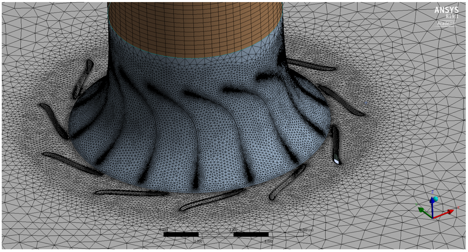
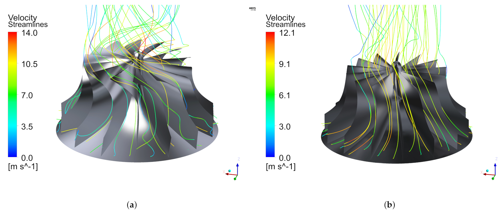
A CAD rendering of the first turbine model is shown in Figure 7a. The resulting CAD geometry was exported to ANSYS for meshing in preparation of CFD analysis as shown in Figure 8. The easiest way to reduce turbine and installation costs is to minimize N. The second design used an inlet angle as defined in Figure 6 of ϕ₁ = 70${}^{\circ }$. N was calculated using Whitfield’s relationship which is Equation (8.31c) from [32]. The result was

$$N={cos}^{-2}{\varphi }_1\approx 9\mathrm{blades}$$

(20)

The number of IGVs in the stator was found using Equation (12) and M = 2, the lowest recommended value.

The third design considers an approximately straight blade profile at the exducer that reduces the stress due to the bending moment caused in large turbines by their own weight. Figure 7c shows that turbine design with 14 blades. The trailing edge has a minimum curvature to reduce the circumferential velocity. N = 14 was used for the first and third turbines to lower the impeller-stator interference as calculated by M compared to $N=9$. CFD simulations will determine if the increase in N is worthwhile.

4. CFD Methodology

4.1. Boundary Conditions, Settings, and Material Properties

Table 2. Boundary conditions.

Location	Type	Description
Bottom of the heat storage layer	Wall	$Ta$ = 296.15 K
Sides of the heat storage layer	Wall	Adiabatic
Collector roof	Semi-transparent wall	h = 15.77 W/(m${}^2$K), $Ta$ = 296.15 K,
		solar irradiation of 850 W/m${}^2$
Chimney wall	Wall	Adiabatic
Collector inlet	Pressure inlet	$P_{\mathrm{gauge}}$ = 0 Pa, $T_a$ = 296.15 K
Chimney outlet	Pressure outlet	$P_{\mathrm{gauge}}$ = 0 Pa
Blades	Wall (MRF)	Adiabatic

provides details for the boundary conditions. Two cell zones were created, one as fluid for air, and one as solid for the ground of the collector which in this case is soil. A heat storage layer thickness of 5 m was used [33]. The heat transfer coefficient for the collector was computed using Equation (4.5) from Burger [34]; it was used in previous SCPP studies because it was developed for wind speeds between 0 and 5 m/s in asphalt pavement samples (horizontal surfaces as the collector in an SCPP). According to data from [28] for Manzanares which is located at latitude 39.04286 and longitude −3.253375 (GMT +1), the wind at noon on September 2nd of a typical year was 14 km/h. The heat transfer coefficient is

$$h=3.87+0.0022v_w\rho C_p{\left(\mu C_p/k\right)}^{-2/3}=15.6\mathrm{W}/({\mathrm{m}}^2\mathrm{K})$$

(21)

The basic settings of the CFD simulation and material properties were taken from Gholamalizadeh and Kim [15] and are listed in

Table 3. Basic settings of the CFD simulation.

Classification	Setting
Solver	Pressure-based coupled algorithm 3-D simulation
	Steady state analysis (second-order upwind discretization)
Rotating reference frame	MRF
Energy equation	Activated
RANS model	RNG k-$\epsilon$ model
	Full buoyancy effects
Radiation model	DO (discrete ordinates)
	Theta divisions: 3
	Phi divisions: 5
	Theta pixels: 3
	Phi pixels: 5
Solar load model	Solar ray tracing

and Table A2 in Caicedo [18].

4.2. Choice of Turbulence Model and Grid Convergence Study

This study was done using rotationally symmetric flow passage around a single blade without IGVs for the first design which was meshed using TurboGrid. The RNG k-$\epsilon$ with wall functions and SST $k-\omega$ turbulence models were used to evaluate the change in power by changing the turbulence model; for this grid 10 < $y^{+}$ < 260. Two other grids were built with 0.2 < $y^{+}$ < 26 and 0.1 < $y^{+}$ < 19, with a prism layer growth rate down to ≅ 1.2; both grids have approximately the same $y^{+}$ range. The last two grids solve the viscous sublayer. See [18] for $y^{+}$ distribution over the blade.

Table 4. Grid convergence study for a flow passage around a blade using different turbulence models and numbers of cells.

Mesh	No. of Cells	Power (kW)	Turbulence Model	${\mathit{y}}^{+}$ Range
Coarse (3)	570,000	81.63	RNG k-$\epsilon$	10–260
Coarse (3)	570,000	83.02	SST $k-\omega$ $k-\omega$	10–260
Medium (2)	1.9 million	80.24	SST $k-\omega$ $k-\omega$	0.2–26
Fine (1)	6.5 million	79.11	SST $k-\omega$ $k-\omega$	0.1–19

presents the results for different grids with a refinement ratio of 1.5. The difference in power between the RNG k-$\epsilon$ and SST $k-\omega$$k-\omega$ model is around 1.7%. It is concluded that the turbulence model does not have a big effect on the calculated turbine efficiency. The decrease in power as the mesh is refined agrees with the CFD results for the 3D turbine model, thus it is not necessary to solve the viscous sublayer and the RNG k-$\epsilon$ turbulence model with scalable functions is a good approximation for the whole domain.

The theory in [35] was applied to assess grid convergence. The order of convergence p can be obtained using three solutions (f${}_1$ to f${}_3$), where f was chosen to be the variable of study for each grid. The constant grid refinement ratio r in 3D is the cube root of the ratio of the numbers of cells in grids 1 and 2 and 2 and 3

$$p=\ln \left(\frac{f_3-f_2}{f_2-f_1}\right)/\ln \left(r\right)$$

(22)

The estimation of the true value is performed using Richardson extrapolation for $f_{h=0}$ which is the limiting value at zero grid spacing

$$f_{h=0}\cong f_1+\frac{f_1-f_2}{r^p-1}$$

(23)

The percentage difference between the computed value and the asymptotic value is the grid convergence index ($GCI$). A small $GCI$ indicates that the computation is within the asymptotic range. It is calculated in two steps, from grids 3 to 2 and from 2 to 1. The equation to compute the $GCI$ is

$$GCI=\frac{F_s\left|\epsilon \right|}{r^p-1}$$

(24)

where F_s is a safety factor recommended to be 1.25 for comparisons over three or more grids and $\epsilon$ is the error between two grids.

5. Results

Four configurations were simulated: the updraft tower without a turbine to get the maximum power that can be extracted, and the SCPP with a turbine for designs 1 to 3 to calculate the maximum power output. Grid convergence studies were undertaken for the updraft without a turbine and the SCPP with the first turbine design.

5.1. The SCPP Available Power

The maximum power without a turbine is the kinetic energy converted from the pressure difference to accelerate the air. CFD results are listed in

Table 5. Grid convergence study for SCPP without turbines.

Mesh	No. of Cells	Mass Flow Rate (kg/s)	Upwind Velocity (m/s)	Kinetic Energy (kW)
Coarse (3)	1 million	1019	11.7	70
Medium (2)	2.7 million	1044	12.0	75
Fine (1)	7.4 million	1060	12.1	78
Richardson Extrapolation		1088	12.5	85

for different numbers of cells. The upwind velocity was calculated at the outlet using the mass flow rate value from the area-weighted average.

These values were used to check whether the solutions are in the asymptotic range of convergence using

$$\frac{GC{I}_{23}}{r^p\times GC{I}_{12}}=1.015\cong 1$$

(25)

The value is approximately one, which indicates that the solutions are within the asymptotic range of convergence. Gholamalizadeh and Chung [31] studied the performance of the Manzanares turbine with a final mesh size of 5.2 million, and the results showed that the maximum power (63.6 kW) could be achieved at 140 rpm. If the actual efficiency is considered ($\eta$_t = 0.83) [13], the maximum power that could be extracted is around 77 kW. This value is between the output power for 2.7 and 7.4 million cells in the present study. Using the same grid convergence analysis for the velocity and the maximum power, the Richardson extrapolated values are 12.5 m/s and 85 kW, respectively.

5.2. SCPP with a Turbine

It was stated on Equation (17) that the maximum angular velocity is determined by the specific speed. The value that maximizes the power will be obtained in this section using MRF and varying the angular velocity of the rotor. It is necessary to model the whole 3D domain instead of one flow passage around a single blade because N and n are not equal; thus, the interfaces between the rotor and stator do not match. Further, the chimney causes a shadow on the collector, which also prevents rotational symmetry. The shadow represents approximately 2% of the collector area and so can be ignored; therefore, the main reason to undertake a full simulation is the difference between N and n of the turbine with IGVs.

The output power is calculated on the medium grid at different rotational speeds (see Figure 9). At rotational speeds higher than 15 rpm, there is backflow in the turbine and its efficiency reduces. Thus, the convergence analysis was performed at 15 rpm. Three grids and their data are listed in

Table 6. Grid convergence study for first turbine at $\Omega$ = 15 rpm.

Mesh	No. of Cells	Mass Flow Rate (kg/s)	Torque (Nm)	Power (kW)
Coarse (3)	5 million	476	44,520	70
Medium (2)	7.2 million	477	42,780	67.2
Fine (1)	10.4 million	479	42,250	66.4
Richardson Extrapolation		516	42,020	66

.

Figure 9 also relates to an important point raised by one of the reviewers: what are the cut-in and cut-out speeds of the RIF turbine? Initially, it was thought that these would be unimportant on the grounds that the turbine would normally start and stop at most once per day. That assumption, however, is likely to be true only for a desert-like climate with excellent winter insulation. A full analysis of the unsteady turbine performance would require detailed time-dependent weather data and an unsteady simulation, which would require a much more comprehensive analysis than that presented here.

This gives a power output of 66 kW at 15 rpm for the first design, which is equivalent to an efficiency of 78%. The mass flow rate is lower than the values presented in Table 5 because the turbine acts as a restrictor. The reported power of the Manzanares prototype was 36 kW. Gholamalizadeh and Chung [31] found that the maximum power of an axial turbine is 63.6 kW at 140 rpm.

The torque for the second design is 30.43 kNm and the power is 31.8 kW at 10 rpm. This represents a significant reduction in output power, as N was reduced from 14 to 9. There is backflow above 10 rpm, which means that the equation to determine the number of blades by Glassman [30] is a better fit for this turbine. The minimum number of blades is directly proportional to the angular velocity.

The mass flow rate in the third design is 582 kg/s; it is higher than the mass flow rate for the first design presumably because of the interaction between the changed outlet geometry and the overall SCPP flow. This is illustrated in Figure 10a,b, where the streamlines are shown for an observer rotating with the blades. As the first turbine has backward facing blades, which cause the blockage, its downstream swirl should be lower than for the third design, which should influence the efficiency. The third turbine’s high efficiency is partly a consequence of the $\Omega$. The specific speed for design three is 2.5 rad, the torque is 49,470 Nm, and the power at 15 rpm is 77.7 kW with an efficiency of 91.9%. This efficiency is comparable to the best achieved by other turbine types in the literature. FEA simulations were performed in [18] to determine the safe blade thickness for each design.

6. Conclusions

This paper describes the first study of a radial inflow (RIF) turbine for use in a solar chimney power plant (SCPP). The motivation is that the turbines for SCPPs are unlikely to be mass produced, so a design that is easily and cheaply produced will reduce the significant cost of the turbine. A collateral benefit is that the generator is located at ground level, which is desirable in terms of mounting. Three turbine designs are presented. The blades for the third turbine could be rolled from a metal sheet or easily manufactured using fiberglass; the other two using fiberglass. These turbines were designed for the Manzanares SCPP to assess the feasibility of RIF turbines in terms of the maximum efficiency. The other features of the design and CFD were:

• The software CFturbo 10.3 was used to design the blade profile for three turbines. CFD was then applied to assess the final design using multiple reference frames, the renormalization group k-$\epsilon$ turbulence model, and a discrete ordinates radiation model. The IGVs were assumed to be integral to the columns to support the chimney, so their thickness made it necessary to simulate them in conjunction with the turbine.
• Grid convergence analysis was applied to determine the accuracy of the results. Richardson extrapolation values were taken to obtain the power output of the turbines.

The following points summarize the findings:

1

The maximum power of the third design of the radial turbine is 77.7 kW at 15 rpm, which is higher than the maximum power that could be extracted from the Manzanares prototype at 140 rpm, computed to be 63.6 kW, and is comparable to the most efficient designs of other turbine types in the literature. CFD calculations show that straight blades in a radial turbine have better performance because they reduce the flow restriction on the rotor outlet.

2

Comparison was made between two turbulence models. It was shown that the power output changed by less than 1.7% when the turbulence model was changed from RNG k-$\epsilon$ to SST $k-\omega$, so the turbulence model does not have a big impact on predicted performance.

3

CFturbo proved invaluable as the initial design tool for the turbine blades and IGVs. It allows control of all the dimensions and curvatures in the trailing edge and leading edge.

Future work on turbine design could determine whether a straight-bladed turbine has equally high efficiency, and whether composite materials can be used to build larger thin blades to get more power out of a SCPP with larger dimensions than the Manzanares prototype. From the discussion of Figure 9, it is likely that detailed unsteady simulations of the turbine and SCPP will be needed to finalize the design.

References

1. Haaf, W.; Friedrich, K.; Mayr, G.; Schlaich, J. Solar Chimneys Part I: Principle and Construction of the Pilot Plant in Manzanares. Int. J. Sol. Energy 1983, 2, 3–20. [Google Scholar] [CrossRef]
2. Fluri, T.P.; Von Backström, T.W. Performance analysis of the power conversion unit of a solar chimney power plant. Sol. Energy 2008, 82, 999–1008. [Google Scholar] [CrossRef]
3. Gannon, A.J.; Von Backström, T.W. Solar Chimney Turbine Part 1 of 2: Design. In Proceedings of the International Solar Energy Conference, Reno, NV, USA, 15–20 June 2002; ASME: Matieland, South Africa, 2002; pp. 335–341. [Google Scholar] [CrossRef]
4. Gannon, A.J.; Von Backström, T.W. Solar Chimney Turbine Part 2 of 2—Experimental Results. In Proceedings of the International Solar Energy Conference, Reno, NV, USA, 15–20 June 2002; ASME: Matieland, South Africa, 2002; pp. 343–349. [Google Scholar] [CrossRef]
5. Von Backström, T.; Gannon, A. Solar chimney turbine characteristics. Sol. Energy 2004, 76, 235–241. [Google Scholar] [CrossRef]
6. Dehghani, S.; Mohammadi, A.H. Optimum dimension of geometric parameters of solar chimney power plants—A multi-objective optimization approach. Sol. Energy 2014, 105, 603–612. [Google Scholar] [CrossRef]
7. Denantes, F.; Bilgen, E. Counter-rotating turbines for solar chimney power plants. Renew. Energy 2006, 31, 1873–1891. [Google Scholar] [CrossRef]
8. Tingzhen, M.; Wei, L.; Guoling, X.; Yanbin, X.; Xuhu, G.; Yuan, P. Numerical simulation of the solar chimney power plant systems coupled with turbine. Renew. Energy 2008, 33, 897–905. [Google Scholar] [CrossRef]
9. Rangel, L.P.; Contessi, B.A.; Copes, T.A.; Alberto, P.; Ropelato, K. Advances in solar chimney turbine modelling. Asociación Argentina de Mecánica Computacional 2016, XXXIV, 897–915. [Google Scholar]
10. Zhou, Y.; Gao, B.; Dong, H.R.; Hao, K. Design for the turbine of solar chimney power plant system with vertical collector. IOP Conf. Ser. Earth Environ. Sci. 2016, 40, 012085. [Google Scholar] [CrossRef] [Green Version]
11. Fluri, T.P. Turbine Layout for and Optimization of Solar Chimney Power Conversion Units. Ph.D. Thesis, University of Stellenbosch, Stellenbosch, South Africa, 2008. [Google Scholar]
12. Elmagid, W.M.; Keppler, I. Axial flow turbine for solar chimney. Hung. Agric. Eng. 2017, 32, 29–37. [Google Scholar] [CrossRef]
13. Haaf, W. Solar Chimneys Part II: Preliminary Test Results from the Manzanares Pilot Plant. Int. J. Sol. Energy 1984, 2, 141–161. [Google Scholar] [CrossRef]
14. Gholamalizadeh, E.; Chung, J.D. A Comparative Study of CFD Models of a Real Wind Turbine in Solar Chimney Power Plants. Energies 2017, 10, 1674. [Google Scholar] [CrossRef] [Green Version]
15. Gholamalizadeh, E.; Kim, M.H. Three-dimensional CFD analysis for simulating the greenhouse effect in solar chimney power plants using a two-band radiation model. Renew. Energy 2014, 63, 498–506. [Google Scholar] [CrossRef]
16. Zhang, X.; Wang, P.; Ruan, X.; Xu, Z.; Fu, X. Analysis of Pressure Pulsation Induced by Rotor-Stator Interaction in Nuclear Reactor Coolant Pump. Shock Vib. 2017, 2017, 7363627. [Google Scholar] [CrossRef] [Green Version]
17. Liu, J.; Tian, R.; Nie, J. Design of Wind Turbine Blade for Solar Chimney Power Plant. J. Shanghai Jiaotong Univ. (Sci.) 2018, 23, 820–826. [Google Scholar] [CrossRef]
18. Caicedo, P.V. Feasibility Study of a Radial Turbine for a Solar Chimney Power Plant. Master’s Thesis, University of Calgary, Calgary, AB, Canada, 2018. [Google Scholar] [CrossRef]
19. Kasaeian, A.; Molana, S.; Rahmani, K.; Wen, D. A review on solar chimney systems. Renew. Sustain. Energy Rev. 2017, 67, 954–987. [Google Scholar] [CrossRef]
20. Ferziger, J.H.; Peric, M. Computational Methods for Fluid Dynamics, 3rd ed.; Springer: Berlin, Germany, 2002; p. 423. [Google Scholar] [CrossRef]
21. Bergman, T.L.; Lavine, A.S. Fundamentals of Heat and Mass Transfer; Wiley: Lawrence, NY, USA, 2017; ISBN ES8-1-119-32042-5. [Google Scholar]
22. Andersson, B.; Andersson, R.; Håkansson, L.; Mortensen, M.; Sudiyo, R.; Van Wachem, B. Computational Fluid Dynamics for Engineers; Cambridge: Cambridge, UK, 2011; Volume 9781107018, pp. 1–189. [Google Scholar] [CrossRef] [Green Version]
23. Ansys, I. Fluent Theory Guide; ANSYS: Canonsburg, PA, USA, 2020. [Google Scholar]
24. Duffie, J.A.; Beckman, W.A. Solar Engineering of Thermal Processes, 4th ed.; Wiley: New York, NY, USA, 2013. [Google Scholar]
25. Luo, J.Y.; Issa, R.I.; Gosman, A.D. Prediction of Impeller Induced Flows in Mixing Vessels Using Multiple Frames of Reference; IChemE Symposium Series; Institute of Chemical Engineers: New York, NY, USA, 1994. [Google Scholar]
26. CFturbo GmbH. CFTurbo; Dresden, Germany, 2018. Available online: https://manual.cfturbo.com/en/index.html (accessed on 20 December 2020).
27. Rohlik, H.E. Analytical Determination of Radial Inflow Turbine Design Geometry for Maximum Efficiency; NASA: Washington, DC, USA, 1968. [Google Scholar]
28. World Weather Online. World Weather Online, 2008. Available online: https://www.worldweatheronline.com/manzanares-weather-history/castilla-la-mancha/es.aspx (accessed on 20 December 2020).
29. López, E. Study on a Radial Turbine Stage with Inlet Guide Vanes for an ORC Process with an Electrical Output of 3, 5 kW; Final Project; Universität Stuttgart: Stuttgart, Germany, 2013. [Google Scholar]
30. Glassman, A.J. Computer Program for Design Analysis of Radial-Inflow Turbines; NASA: Washington, DC, USA, 1976. [Google Scholar]
31. Gholamalizadeh, E.; Chung, J.D. Analysis of fluid flow and heat transfer on a solar updraft tower power plant coupled with a wind turbine using computational fluid dynamics. Appl. Therm. Eng. 2017, 126, 548–558. [Google Scholar] [CrossRef]
32. Dixon, S.L.; Hall, C.A. Fluid mechanics and Thermodynamics of Turbomachinery; Elsevier: Waltham, MA, USA, 2014. [Google Scholar] [CrossRef]
33. Gholamalizadeh, E.; Kim, M.H. CFD (computational fluid dynamics) analysis of a solar-chimney power plant with inclined collector roof. Energy 2016, 107, 661–667. [Google Scholar] [CrossRef]
34. Burger, M. Prediction of the Temperature Distribution in Asphalt Pavement Samples. Master’s Thesis, University of Stellenbosch, Stellenbosch, South Africa, 2005. [Google Scholar]
35. NASA. Examining Spatial (Grid) Convergence; NASA: Washington, DC, USA, 2008.
Figure 1. Sectional view of a solar chimney power plant (SCPP) with an axial turbine in the chimney, adapted from [6]. The dimensions are: D 1 = D 2 = 10 m, H 1 = H 2 = 1.85 m, and H C = 194.6 m.
Energies 14 00674 g001
Figure 2. Configurations of axial turbines in an SCPP; (a) single vertical axis (VA) turbine, (b) multiple VA turbines, and (c) multiple horizontal axis (HA) turbines from Fluri [2].
Energies 14 00674 g002
Figure 3. Schematic drawing of turbine layouts, adapted from [11].
Energies 14 00674 g003
Figure 4. Schematic of the proposed radial turbine using Manzanares SCPP dimensions.
Energies 14 00674 g004
Figure 5. Main geometrical features of the radial inflow (RIF) blade.
Energies 14 00674 g005
Figure 6. Velocity triangles for an RIF turbine with radial inlet flow and axial outlet flow adapted from [29]. C 0 is the radial flow into the turbine located at the base of the chimney. The numbers on the left indicate the turbine sections.
Energies 14 00674 g006
Figure 7. 3D model of the stator and rotor completed in CFturbo for the three designs. Direction of rotation—counterclockwise. (a) First design; (b) second design; (c) third design.
Energies 14 00674 g007
Figure 8. Grid completed in ANSYS Meshing using the 3D turbine model.
Energies 14 00674 g008
Figure 9. Variation in the power output with the turbine rotational speed for the first design.
Energies 14 00674 g009
Figure 10. Streamlines in rotating co-ordinates for the first and third designs. Direction of rotation—counterclockwise. (a) Streamlines for the first design; (b) streamlines for the third design.
Energies 14 00674 g010