Abstract
A Monte Carlo simulation methodology is suggested in order to assess the impact of ambient wind on a vehicle’s performance and emissions. A large number of random wind profiles is generated by implementing the Weibull and uniform statistical distributions for wind speed and direction, respectively. Wind speed data are drawn from eight cities across Europe. The vehicle considered is a diesel-powered, turbocharged, light-commercial vehicle and the baseline trip is the worldwide harmonized light-duty vehicles WLTC cycle. A detailed engine-mapping approach is used as the basis for the results, complemented with experimentally derived correction coefficients to account for engine transients. The properties of interest are (engine-out) NO and soot emissions, as well as fuel and energy consumption and CO2 emissions. Results from this study show that there is an aggregate increase in all properties, vis-à-vis the reference case (i.e., zero wind), if ambient wind is to be accounted for in road load calculation. Mean wind speeds for the different sites examined range from 14.6 km/h to 24.2 km/h. The average increase in the properties studied, across all sites, ranges from 0.22% up to 2.52% depending on the trip and the property (CO2, soot, NO, energy consumption) examined. Based on individual trip assessment, it was found that especially at high vehicle speeds where wind drag becomes the major road load force, CO2 emissions may increase by 28%, NO emissions by 22%, and soot emissions by 13% in the presence of strong headwinds. Moreover, it is demonstrated that the adverse effect of headwinds far exceeds the positive effect of tailwinds, thus explaining the overall increase in fuel/energy consumption as well as emissions, while also highlighting the shortcomings of the current certification procedure, which neglects ambient wind effects.
1. Introduction
Much attention has been paid lately to real-world driving emissions from passenger cars and commercial vehicles. The difference between real-world and type-approval values for fuel consumption and emissions peaked at almost 42%, on average, in 2016 [1]. Since then, there has been some decline, although the gap is far from closed [2], and recent studies show that the newly adopted Worldwide-harmonized Light-duty Test Procedure (WLTP) alone will not be able to bridge that gap [3]. When it comes to light commercial vehicles, their contribution to aggregate transport emissions is expected to come under the spotlight, as home-delivery practices become all the more widespread [4,5,6], with the COVID-19 crisis further accelerating this trend.
One significant contributor to the gap between real-world and type-approval emissions, accounting for more than one-third of it, is the under-estimation of real-world road load forces, namely rolling resistance, aerodynamic drag, and gradient resistance [7,8,9]. To make matters worse, the latter is entirely excluded, mostly for practical reasons, from road load determination during type-approval testing, although its effect on emissions is far from negligible even for a zero net elevation trip [10,11,12,13,14,15].
Another hugely important variable of the real-world driving environment is natural wind and its fluctuations in terms of velocity as well as direction with respect to the vehicle movement. During a typical trip, both wind velocity and wind direction can vary significantly depending on the surroundings, the presence of other vehicles on the road, the appearance of wind gusts, etc. [16]. On the contrary, the aerodynamic development of vehicles typically takes place in wind tunnels or with the use of CFD techniques assuming ideal conditions (e.g., uniform flow), thus introducing discrepancies vis-à-vis the actual aerodynamic performance of a vehicle driven on the road [17,18,19].
Such discrepancies are amplified by the exclusive use of the zero-yaw drag coefficient to determine the vehicle’s aerodynamic performance. The zero-yaw drag coefficient represents the minimum drag condition for a vehicle, with the actual drag experienced by a vehicle expected to rise considerably as a function of the yaw angle [20].
The WLTP provides alternatives with regards to the determination of aerodynamic drag as part of the total road load. On the one hand, the vehicle can be tested in a wind tunnel assuming minimum levels of turbulence and zero yaw [21,22]. On the other hand, the vehicle may undergo a coast-down test in order to determine the road load coefficients for use in dynamometer setting. During this procedure, the vehicle is driven on a flat and dry test track, and average wind speeds do not exceed 3 m/s. The test is conducted in both directions, and the net effect of wind is further eliminated by a relevant wind correction algorithm [23,24,25]. In both cases, natural wind and its effect on vehicle performance and emissions is neglected. The opposite is true for the RDE procedure, as there is no limit on the permissible value for ambient wind speed throughout a trip [23]. However, the RDE procedure focuses on NOx and particle number, not yet accounting for fuel consumption/CO2 emissions [26].
The concept of the wind-averaged drag was introduced as early as the 1970s, with the aim of providing a more accurate representation of the real-world aerodynamic performance of a vehicle [27]. Initial studies were limited to vehicle operation at constant speed but quickly the focus shifted to driving schedules [28]. Several methods have been suggested so far with regards to the derivation of the wind-averaged drag coefficient, all of them considering different distributions of vehicle speed, wind speed, and wind direction relative to the vehicle movement [20]. Recent studies [22,29] applied the wind-averaged drag concept in the context of homologation cycles, including the WLTC as well as EPA drive cycles (FTP, HWFET, US06, SC03), relying on meteorological data for a particular region (e.g., the UK or Western Europe, in general) to derive a reference wind speed for the calculations.
The present study aims to expand on the above methodologies by implementing a Monte Carlo simulation methodology to generate a large number of random wind speed and direction profiles, based on appropriate statistical distributions derived from wind speed data for different cities around Europe. What is more, the scope of study is also expanded to include engine-out pollutants and energy consumption. The driving schedule used to assess the impact of the aforementioned wind profiles on performance and emissions is the worldwide harmonized light-duty vehicles test cycle—WLTC. This allows for a direct comparison to the type-approval case, i.e., no wind. Calculations are performed with the use of a detailed vehicle and engine model that was detailed in previous publications by the present research group [30,31].
The distinctive advantage of the proposed methodology that sets it apart from previous studies is that instead of relying on a suitable correction to be applied on the vehicle’s drag coefficient across the whole cycle (in order to account for real-world aerodynamic performance), here the drag coefficient is calculated on a second-by-second basis, based on the instantaneous values of wind speed and direction, as well as vehicle speed. By doing so, useful correlations between wind speed and direction, on the one hand, and fuel/energy consumption and emissions on the other, can be derived, allowing for the effect of engine transients on emissions (not limited to CO2 but covering pollutants, too, namely soot and NO) to be further highlighted. What is more, a comparison between the methodology presented herein and the cycle-averaged drag coefficient method, presented in Howell et al. [22], is also carried out.
2. Materials and Methods
2.1. Impact of Ambient Wind on Aerodynamic Drag
When a vehicle is driven on the road with a vehicle speed , in the presence of a natural wind blowing with velocity and direction θ, the relative air speed (Figure 1) is as follows:
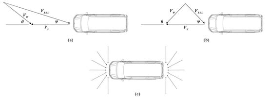
Figure 1.
(a) Velocity triangle for headwind, (b) Velocity triangle for tailwind, (c) Headwinds and tailwinds approaching the vehicle equiprobably.
The relative air speed creates an angle ψ with the vehicle direction of movement. This is called the yaw angle and is given as follows:
Finally, the aerodynamic drag on the vehicle due to the presence of the ambient wind is
where ρ is the ambient air density, A is the vehicle frontal area, and is the aerodynamic drag coefficient as a function of the yaw angle ψ.
The relative change in the vehicle drag coefficient vis-à-vis the yaw angle is shown in Figure 2, normalized with respect to the drag coefficient at zero yaw. The relevant data were drawn from Heisler [32]. It was assumed that the vehicle was symmetrical around the X-axis, and thus the curve in Figure 2 was symmetrical around .
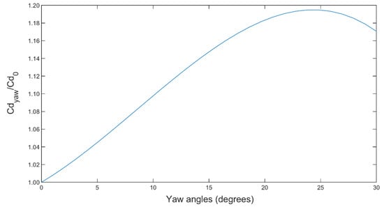
Figure 2.
Increase in the drag coefficient with respect to the yaw angle.
It was noted that the increase of over reached a maximum value at , then started decreasing slowly. Following Sovran [28], we expected that as the yaw angle increased, the drag coefficient would eventually become equal to zero at some yaw angle . A further increase in yaw angle would then see the drag coefficient assuming negative values corresponding to an “aerodynamic push” on the vehicle. Unfortunately, most investigations on the change of drag coefficient with respect to yaw angle were limited to yaw angles of less than 30°, assuming that larger yaw angles were unlikely. In the context of the present study, a cap was imposed on instances of the WLTC where . This was to avoid errors from over-extrapolation, given the lack of data for large yaw angles.
2.2. Generation of Random Wind Profiles
Random wind profiles were generated using the Weibull distribution with respect to wind speed. The Weibull distribution is the most commonly used probability distribution function with respect to the assessment of the wind energy potential of a given area [33,34,35]. The Weibull probability density function is as follows:
where is the probability of observing wind speed , k is the dimensionless shape factor, and c (m/s) is the scale parameter. The mean wind speed can be calculated based on the k and c values as follows:
where Γ is the gamma function.
Data for the Weibull distributions used in this study were drawn from the European Wind Atlas [36]. The European Wind Atlas categorizes data for each site according to three different roughness classes over land. Those roughness classes correspond to different terrain surface characteristics and are defined by the relevant surface roughness length . Table 1 shows the roughness class categorization, including the relevant WLTC phase that can be assumed to exhibit similar terrain characteristics.

Table 1.
Terrain surface characteristics, roughness classes, and roughness lengths for each WLTC phase (data from [35]).
From the roughness classes presented in Table 1, the European Wind Atlas provided data for classes 1 to 3. Weibull distribution parameters for roughness class 4 (city center—low phase of the WLTC) were extrapolated from the tabulated values using Equations (6)–(8) [36], assuming a surface roughness length :
In the above equations, subscripts a and b refer to roughness lengths and Weibull parameters for roughness classes 2 and 3, respectively.
Eight different sites were considered, all of them located near major urban centers that could be assumed to exhibit similar driving conditions to the WLTC phases. Those sites were picked from various regions across Europe, exhibiting different scale and shape parameters for the relevant Weibull probability distribution functions. It was generally observed that for sites in Northern Europe, the shape factor k was close to 2.00; therefore the one-parameter Rayleigh distribution could also be used instead of the two-parameter Weibull one [36].
Table 2 presents geographical data for the sites considered in this study, whereas Table 3 summarizes the scale and shape parameters applicable to each cycle phase and for each site. It is noted here that the altitude of each site was not considered in the calculations and is only listed here for reference. The same goes for other climatological data (e.g., temperature). Such a full-blown investigation of the wind drag components fell out of the scope of the present study.
Table 2.
Geographical data for the eight sites considered (data from [35]).
Table 3.
Weibull scale factor c and shape factor k for the eight sites considered (data from [35]).
It is noted that these Weibull distribution parameters corresponded to a wind blowing at 10 m above ground. This wind speed was then corrected to the vehicle height using the logarithmic law [37,38]. Following Howell et al. [29], we considered to be equal to , where VH is the vehicle height.
With regards to wind direction, the uniform distribution was chosen with min = and max =. This is consistent with most approaches regarding wind-averaged drag calculation that assume equiprobable wind direction in the range of to [20]. The same approach was taken by Khayyam [39] and validated via a Pearson chi-square test against empirical data.
Once the statistical distributions for wind speed and direction were defined, the generation of random profiles proceeded by picking a random wind speed for each cycle phase from the relevant Weibull distribution for each of the sites examined. Then a random wind direction was picked for each of the phase segments. The low and medium phases were broken down to 10 and 8 segments, respectively, whereas for the high and extra-high phases, the number of segments was 5 and 3, respectively (see Figure 3). This was done in order to reflect the influence of traffic conditions, as well as road geometry for the different type of roads that each cycle phase represented (city center, extra-urban, rural, and highway).
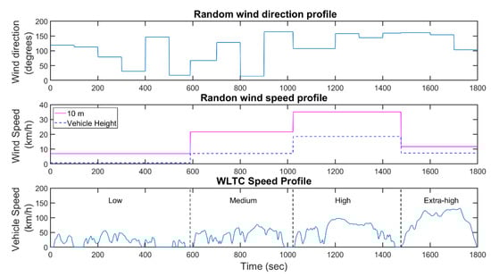
Figure 3.
Random WLTC wind profile.
Finally, the diurnal wind speed variation was also taken into account. The European Wind Atlas [36] presents data on the mean annual observed wind speeds at different hours of the day for each site, with a three-hour step. A light commercial vehicle is typically expected to be driven in the hours between 06:00 and 18:00; therefore a correction factor was applied to each random wind speed, following the below formula for each site:
Correction factors for the wind diurnal variation are included in the rightmost column of Table 3. It was noted that sites in Southern European regions exhibited higher diurnal correction factors as opposed to Northern European ones.
2.3. Experimental Investigation and Engine Modeling
For each of the random wind profile WLTC trips, generated based on the methodology described above, instantaneous emissions from a diesel-powered, turbocharged, light-commercial vehicle were calculated with the use of an integrated engine and vehicle model. This model formed the basis of previous publications of the present research group [30,31] and is briefly discussed here for the sake of completeness.
The engine model was built based on a combined experimental/computational approach. The context of quasi-linear modeling was adopted for the most part, in a similar fashion to previous mapping-based studies [40,41]. The starting point for the model was the steady-state experimental investigation of the engine at hand; polynomial expressions were derived for each of the properties of interest vis-à-vis instantaneous engine load and speed [42]. With regards to engine power, as well as fueling and CO2 emissions, this approach was expected to provide accurate results.
However, that was not the case for NO and soot emissions (also investigated in the present study), mostly due to the effect of turbocharger lag. The latter is strongly related to engine transient events (accelerations and load changes) and can result in significant overshoots for NO and soot emissions [43,44], which a mapping-based approach can easily overlook. Thus, on top of the steady-state mapping of the engine, a detailed transient investigation was also carried out, focusing on transient events similar to the ones encountered during a typical transient driving schedule. Fast-response analyzers were used, enabling the derivation of correction coefficients for both NO and soot based on the magnitude of the transient event [30].
NO was chosen for the present analysis since it forms the biggest part of NOx emissions from diesel engines [45,46]. On the other hand, soot was studied as surrogate to particulate matter, which is very hard to measure instantaneously [47]. For all results presented herein, it was assumed that the engine was fully warmed up, i.e., no cold-start effects were taken into account. Lastly, it is noted that all emitted pollutants referred to engine-out conditions.
2.4. Integrated Engine and Vehicle Model
Coupled to the engine model was a detailed vehicle model capturing instantaneous vehicle longitudinal dynamics based on Equation (11) [32,48]:
Tractive force needs to be exerted on the wheels by the engine in order for the vehicle to overcome the sum of forces applied to it, including rolling resistance , aerodynamic resistance, gradient resistance , and inertia resistance . In the above equation, is the rolling resistance coefficient, is the vehicle mass, g is the gravitational acceleration, and α is the road slope angle. The rolling resistance coefficient was calculated on a second-by-second basis using a detailed mass-spring and damper model to account for tire hysteretic behavior, which is the biggest contributor to rolling resistance losses [49,50]. Tire micro-slippage, as well as tire windage losses, were also considered in the estimation of the rolling resistance coefficient [31].
The gradient angle was set to zero for the whole duration of the driving schedule in order to isolate ambient wind effects. The term MF is the mass factor and was included in the calculation of the inertia resistance to represent the inertia of the driveline rotating components. It is calculated using Equation (12) [48]:
With regards to instantaneous engine speed , we have
where is the instantaneous wheel angular speed, is the tire dynamic radius, is the back-axle transmission ratio, and is the gear transmission ratio.
The tire dynamic radius is defined as the ratio between the vehicle forward speed and the wheel angular speed. Its value sits somewhere between the tire unloaded or geometric radius and the tire static radius. The latter is a function of tire dimensions as well as inflation pressure [51,52], whereas the former is a design feature of the tire. The three radii are related as per Equation (14) [53]:
The instantaneous engine load is
is the auxiliaries power (lighting, A/C, radio, etc.), which was also taken into account.
Instantaneous drivetrain losses are estimated based on Equation (16) below [54]:
where NG is the total number of forward gears used and is the gear used at each second of the cycle. The latter was defined following the procedure detailed in the WLTP technical specifications [21].
Once the instantaneous engine speed and torque were defined, fuel/energy consumption was calculated from the steady-state investigation of the engine, as were the steady-state values for NO and soot. Based on the load and speed change, transient correction coefficients were applied to the estimation of NO and soot transient overshoots that, together with the steady-state values, formed the overall NO and soot emissions [30]. Finally, instantaneous values for fuel/energy consumption, CO2, NO, and soot emissions were translated into cumulative, distance-specific values for the WLTC, as well as for the different cycle phases.
The data of the engine and vehicle used for the analysis are summarized in Table 4.
Table 4.
Engine and vehicle data.
2.5. Monte Carlo Simulation Iterations
The purpose of this study was to examine the expected increase in fuel consumption and emissions, vis-à-vis the type-approval case (i.e., no wind), for a light-commercial vehicle driven in an ambient wind environment. Thus, the results are expressed as the percentage rise over the reference case. In order to do so with a certain level of confidence, the central limit theorem (CLT) was implemented [55] in order to define the necessary number of random-wind WLTC trips to be executed.
The CLT states that for a given sample of simulation runs n, the sample mean
has a normal distribution with mean and variance , where μ and S2 are the mean and variance of all possible random-wind WLTC trips, respectively. Typically, the variance S2 is unknown, however it can be estimated with the relevant sample variance for a sufficiently large sample size n (i.e., number of random-wind WLTC trips):
Thus, the (1−α)100% confidence interval can be defined as follows:
where for a 95% confidence interval (α = 5).
The confidence interval can also be expressed as a percentage of the sample mean :
With the aim of estimating with a (i.e., with an accuracy of at least ), an initial sample was taken, of sample size n = 100, to get a rough estimate of mean and variance . Then these values were imported into Equation (20), and we solved for the number of iterations n required for the desired accuracy. For all of the sites considered, a total number of 5000 random-wind WLTC trips was adequate for delivering the desired accuracy.
It is noted that in the analysis above, the individual outcomes of each random-wind trip for all properties of interest are calculated as follows:
Therefore, the final estimates for the expected change in emissions, compared to the reference case, are as follows:
2.6. Cycle-Averaged Drag Coefficient Method
The cycle-averaged drag coefficient (CADC) method has also been discussed in the context of this study [22,29]. The method relies on the wind-averaged drag coefficient methodology, which considers certain values of vehicle speed, as well as wind speed and direction. In the case of a driving schedule, such as the WLTC 3-2 examined here, for each cycle trace the instantaneous wind-averaged drag coefficient is calculated following Equation (29), considering equiprobable wind direction angle :
The relative air speed , as well as the yaw angle , are calculated following Equation (1) and Equation (2), respectively. Having calculated the wind-averaged drag at each cycle trace, the cycle-averaged drag coefficient is then calculated for the whole duration T of the cycle:
The vehicle aerodynamic drag to be used in Equation (11) is then:
In order to get to the cycle-averaged drag coefficient , we needed a reference wind speed, which we obtained by considering the mean wind for each site, based on the relevant Weibull distribution parameters (Table 3).
3. Results and Discussion
3.1. Simulation Results
First, the reference case was simulated assuming an unloaded vehicle (kerb mass plus driver) and zero wind (zero road gradient, too). The results for the reference case are listed in Table 5, including a phase-by-phase breakdown of the cycle.
Table 5.
Distance-specific results for the type-approval case (zero wind).
The estimated increase in fuel/energy consumption and emissions, vis-à-vis the zero-wind case, is tabulated in Table 6 for all sites, including the relevant accuracy of the estimate.
Table 6.
Monte Carlo simulation method results (mean values and standard deviations are %; all other values correspond to rise % over the reference case).
Figure 4 plots the percentage increase against the mean wind for each site, with the aim of providing insight into the relation between the two. This mean wind for each site was taken to be the Weibull mean (see Equation (5)) for the extra-high phase of the cycle at 10 m above ground. The relevant diurnal wind speed correction factor CF (Equation (10)) was also taken into account.
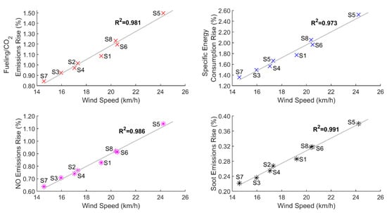
Figure 4.
Expected rise in consumption and emissions vs. mean wind speed.
The windiest site was site 5, with a mean wind speed of 24.2 km/h, whereas the least windy one was site 7, which exhibited a mean wind speed of 14.6 km/h. There was a strong correlation between the percentage rise in emissions and mean wind speed. Specific energy consumption was the property most influenced from the presence of ambient wind, with the percentage increase, vis-à-vis the zero-wind case, being equal to 1.80% on average (max = 2.52%, min = 1.36%, S = 0.38%). Fuel consumption (hence CO2 emissions) followed, with the average increase being 1.10% (max = 1.50%, min = 0.84%, S = 0.22%), whereas NO emissions were modestly increased by 0.83% (max = 1.14%, min = 0.64%, S = 0.16%). Soot was the least influenced property, with its average rise being equal to 0.28%.
Figure 5 plots the increase in all properties of interest with respect to the Weibull scale parameter c (neglecting CF), and Figure 6 does the same, this time with regards to the Weibull shape parameter k. The increase in fuel/energy consumption, as well as NO and soot emissions, correlated well with the scale parameter c (Figure 5), whereas that was not the case at all when it came to the shape parameter k (Figure 6).
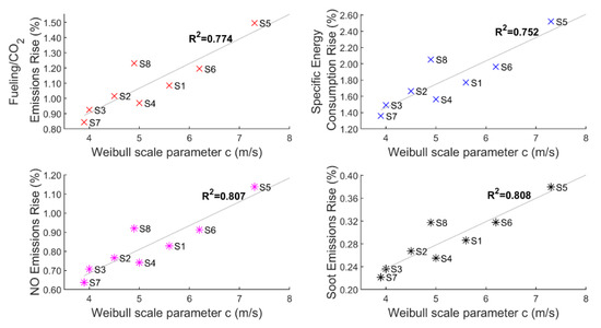
Figure 5.
Expected rise in fuel/energy consumption and emissions vs. Weibull scale parameter c.
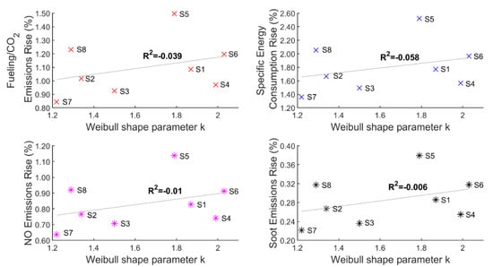
Figure 6.
Expected rise in fuel/energy consumption and emissions vs. Weibull shape parameter k.
3.2. Correlation of Performance and Emissions with Wind Speed and Direction for Individual Trips
The above results give a solid estimate of how much the real-world values for fuel consumption and emissions are expected to vary from the type-approval ones, if the effect of ambient wind is accounted for. In other words, this is the increase that we expect to see from a vehicle being driven in said wind environment over a long period of time. This is not to be confused with the expected increase (or decrease) in consumption and emissions due to wind blowing at a certain speed and direction for an individual trip.
Figure 7, Figure 8, Figure 9, Figure 10, Figure 11, Figure 12, Figure 13 and Figure 14 provide more insight into the latter case. Figure 7, Figure 8, Figure 9 and Figure 10 plot the percentage change in all properties vis-à-vis wind speed, whereas Figure 11, Figure 12, Figure 13 and Figure 14 plot the same change, this time with respect to mean wind direction. The results showcased in the above plots were derived from site 2 and were broken down in the different phases of the WLTC, with the aim of providing more insight into the effect of ambient wind on different vehicle speeds (city center as opposed to highway, etc.).
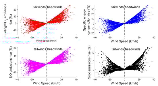
Figure 7.
Percentage increase in consumption and emissions vs. wind speed for the extra-high phase of the WLTC.
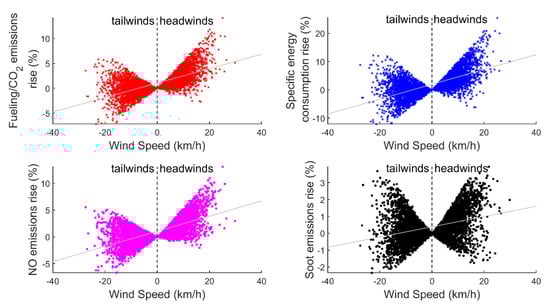
Figure 8.
Percentage increase in consumption and emissions vs. wind speed for the high phase of the WLTC.
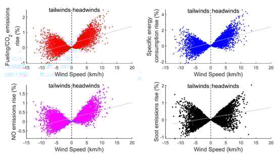
Figure 9.
Percentage increase in consumption and emissions vs. wind speed for the medium phase of the WLTC.
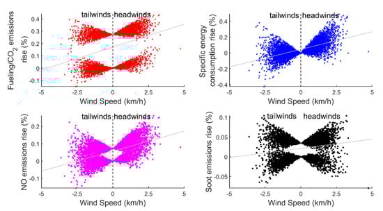
Figure 10.
Percentage increase in consumption and emissions vs. wind speed for the low phase of the WLTC.
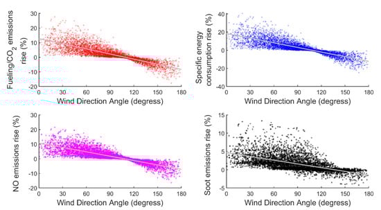
Figure 11.
Percentage increase in fuel/energy consumption and emissions vs. mean wind direction for the extra-high phase of the WLTC.
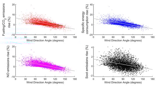
Figure 12.
Percentage increase in fuel/energy consumption and emissions vs. mean wind direction for the high phase of the WLTC.
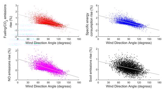
Figure 13.
Percentage increase in fuel/energy consumption and emissions vs. mean wind direction for the medium phase of the WLTC.
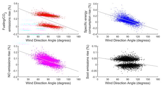
Figure 14.
Percentage increase in fuel/energy consumption and emissions vs. mean wind direction for the low phase of the WLTC.
It is reminded here that the generation of random wind profiles proceeds by picking a single value for wind speed for each cycle phase, whereas for wind direction, each phase is broken down into several segments. Therefore, wind speed in Figure 7, Figure 8, Figure 9 and Figure 10 is the wind speed blowing for the whole duration of each cycle phase, whereas wind direction in Figure 11, Figure 12, Figure 13 and Figure 14 refers to the mean wind direction for the same cycle phase. Idling and deceleration instances of the cycle were discarded in the calculation of mean wind direction, given that wind drag was not contributing to the engine load for the above cases. Moreover, in Figure 7, Figure 8, Figure 9 and Figure 10, “negative” winds correspond to a predominantly tailwind environment (i.e., ), whereas “positive” winds reflect a predominantly headwind environment (). Finally, it is noted that the wind speed referenced in Figure 7, Figure 8, Figure 9 and Figure 10 is the wind blowing at vehicle height and should not be confused with the wind speed at 10 m above ground, referenced in Figure 4.
It is no surprise that the extra-high phase of the WLTC (Figure 7 and Figure 11) exhibited the biggest percentage increases for all properties. Not only were vehicle speeds higher, but the prevailing wind speeds were also higher, due to the different boundary layer characteristics (see Equation (9)). For a wind blowing at 30 km/h (approximately 50 km/h at 10 m reference height) the rise in fueling/CO2 emissions reached 25%, whereas for the specific energy consumption, the equivalent rise was almost 40%. NO emissions for the same case rose up to 21%. Finally, soot, although the most insensitive property with respect to wind for the current engine, still showcased a considerable increase, almost 13%, for the same wind speed. A similar picture is drawn when looking at the high phase of the cycle (Figure 8). For wind speeds above 20 km/h at vehicle height (approximately 40 km/h at 10 m above ground), the increase in fueling/CO2 exceeded 10%, and the same applied to NO emissions.
Focusing on NO emissions, it is noted that higher vehicle speeds, when coupled with strong headwinds, led to increased engine load and therefore higher in-cylinder temperatures, thus favoring the formation of NO [45,56]. The relation between NO emissions and engine load is further illustrated in Figure 15, where the increased NO emissions in the extra-high phase were attributed to the higher operating points, vis-à-vis the reference case, for engine speeds above 2000 rpm.
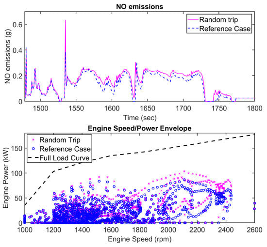
Figure 15.
Engine speed/power envelope (WLTC) and corresponding NO emissions (extra-high phase).
On the other hand, when it comes to soot emissions, it must be clarified that the stated increase happened in a backdrop of relatively low soot emissions for the extra-high phase of the cycle (see Table 5). Therefore, transient events, although instantaneous, can have a relatively big impact on overall soot emissions [57]. It is noted that soot emissions are mostly linked to accelerations from standstill [43,44], typical during city-center driving, where both vehicle and wind speeds (thus aerodynamic drag) are low.
As we moved to the first phases of the cycle, wind speeds, as well as vehicle speeds, were lower and thus the relevant change in all properties of interest was more modest. The maximum rise over the reference case for NO emissions in the low phase of the cycle (Figure 10) was approximately 0.25%, whereas for the soot the maximum rise it was 0.1%. Parameters such as road slope, tire inflation pressure, or auxiliary usage were more prominent in terms of their effect on consumption and emissions for the specific vehicle speed range compared to aerodynamic drag [15,31].
On the other hand, Figure 11, Figure 12, Figure 13 and Figure 14 showcase a generally declining trend for consumption and emissions vis-à-vis wind direction angle. As we gradually moved from a predominantly headwind environment to a predominantly tailwind environment, wind drag on the vehicle and thus engine load and associated fuel/energy consumption and emissions were lowered. However, the decrease in consumption and emissions as we moved towards tailwinds was not enough to offset the relevant increase due to headwinds. Considering the extra-high phase results (Figure 11), where the effect of wind drag was more pronounced, we noted that the maximum increase was 28% for fueling/CO2 emissions, 22% for NO emissions, 13% for soot, and 41% for specific energy consumption. The above numbers correspond to a mean wind direction angle equal to . On the other hand, the minimum values for emissions were observed for a mean wind direction equal to , manifesting an 18% drop in fueling/CO2 emissions, 16% in NO, 4% in soot, and 25% in energy consumption.
The same pattern held true for the rest of the cycle phases (Figure 12, Figure 13 and Figure 14), although for the low and medium phases it was far less pronounced due to vehicle and wind speeds being lower. However, in Figure 12 (high phase) it is shown that there were multiple trips with mean wind direction below , where fueling/CO2 emissions or even NO emissions exhibited a noteworthy increase: above 8% for fueling and NO, and almost 4% for soot. On the contrary, the maximum drop in a tailwind environment was −7.3% for fuel consumption, −6.8% for NO emissions, and −2% for soot.
This fundamental “asymmetry” between the negative effect of headwinds and the positive effect of tailwinds lies behind the findings presented in Figure 4. For a sufficiently large number of trips, the inadequacy of tailwinds to offset the effect of headwinds resulted in a net increase in fuel/energy consumption and emissions, thus highlighting the shortcomings of the current certification procedure, which ignores the effect of ambient wind.
Finally, going back to Figure 11, it is noted that the highest values for consumption and emissions increase did not appear at zero (or close to zero) wind angles, but rather at angles . Going back to Equations (1) and (2) and Figure 1 and Figure 2, we noticed that for such wind angles , the decrease in relative air speed VR compared to the case where (due to was offset from the rise in yaw angle and the subsequent rise in the drag coefficient. This observation challenges the widely accepted notion that vehicle aerodynamics should be optimized for the zero-yaw condition.
3.3. Comparison with the Cycle-Averaged Drag Coefficient Method
The results for the CADC (cycle-averaged drag coefficient) method presented in Section 2.6 are tabulated in Table 7. The difference in the estimated rise compared to the Monte Carlo methodology is included in brackets. In general, the CADC method slightly underestimated the effect of ambient wind on emissions compared to the Monte Carlo method. The discrepancy was more pronounced for soot emissions, although their relative increase vis-à-vis the reference case was rather small in both cases.
Table 7.
Cycle-averaged drag coefficient method result (all values correspond to rise % over the reference case).
Compared to the Monte Carlo method, the CADC method resulted in an estimated 1.04% increase in fueling/CO2 emissions (−5.5% compared to the average Monte Carlo rise), 0.79% in NO (−4.5%), 1.64% in energy consumption (−8.9%), and finally 0.14% soot emissions (−50.0%).
This discrepancy can be attributed to the fundamental difference between the two methods. The cycle-averaged drag coefficient method is a useful and quick tool to assess the impact of a given wind at a given driving schedule [22,29,31]. However, as the name suggests, it relies on replacing the zero-yaw drag coefficient with the cycle-averaged one, which then remains constant throughout the cycle. Contrary to that, the Monte Carlo method suggested in this study calculates the drag coefficient at each second of the cycle (as a function of the yaw angle ψ). By doing so, the aggravation of engine transients due to the instantaneous increase in the wind drag coefficient is allowed to come through.
4. Conclusions
In the present study, fuel and energy consumption, as well as engine-out emissions, were calculated for a light commercial vehicle being driven in a simulated ambient wind environment. This ambient wind environment was constructed by picking random values from the Weibull probability distribution function for wind speed and from the uniform distribution for wind direction. The Weibull scale and shape parameters for the random wind profiles were drawn from eight different sites around Europe. Considering a sufficiently large number of random trips, we arrived at the estimate of the relative increase in fuel/energy consumption and emissions compared to the type-approval case (i.e., zero wind) due to ambient wind presence. The driving schedule employed was the WLTC 3-2.
There was an aggregate increase in all properties, vis-a-vis the reference case (i.e., zero wind), if ambient wind was accounted for in road load calculation. The mean winds for the sites examined ranged from 14.6 km/h to 24.2%. The average fueling/CO2 rise across all sites examined was 1.10% (S = 0.22%), whereas the NO emission average rise was 0.83% (S = 0.16%) and soot emissions exhibited an almost negligible overall increase equal to 0.28% (S = 0.05%). Specific energy consumption was the property most influenced, displaying a 1.80% (S = 0. 38%) increase over the reference case.
However, the above numbers do not tell the whole story. Section 3.2 dug a little deeper by breaking down results from a large number of random trips into the separate phases of the WLTC cycle, i.e., correlations between the change in consumption and emissions on the one hand and wind speed and direction on the other were derived for different vehicle speed regimes. It was shown that for the high and extra-high phases of the cycle, where average vehicle speeds were significantly higher than the low and medium phases (and wind speeds were also expected to be higher as surface roughness decreased), the increase in emissions was much higher, reaching up to 28% for fueling/CO2 emissions, 22% for NO, and 13% for soot in the extra-high phase.
Furthermore, it was noted that although a “tailwind” environment can have a positive effect on the performance and emissions of the vehicle, that effect is not enough to cancel out the adverse effect of a “headwind” environment. Especially with regards to (engine-out) NO and soot emissions, it was found that the instantaneous coupling of a “headwind” with the specific operating point of the engine could greatly affect the overall emissions, even though the overall wind environment may be favorable (i.e., tailwind).
The results from the present study point to the shortcomings of the current homologation procedure, which excludes ambient wind from the calculation of total road load, among other parameters, such as road gradient. Given the technical challenges involved in trying to mechanically simulate the highly dynamic road load in the dynamometer, numerical simulation methodologies such as the one presented herein can prove themselves to be a valuable tool in the effort to accurately capture the real-world performance and emissions of a vehicle. Obviously, real driving emissions testing is expected to play a huge part in that goal, however, simulation is still indispensable, given that a huge number of scenarios can be studied in a fragment of the time and cost involved in RDE testing. What is more, simulation methodologies can further assist engineers in applications such as eco-routing, which, although not directly linked to the challenges of vehicle homologation, can still play a significant role in bringing transportation emissions down.
Author Contributions
A.T.Z. was responsible for the development and execution of the code, as well as the analysis of the results and forming the paper; E.G.G. supervised all the steps of the process and provided the scope for the expansion and better understanding of the work. Both authors have read and agreed to the published version of the manuscript.
Funding
This research received no external funding.
Institutional Review Board Statement
Not applicable.
Informed Consent Statement
Not applicable.
Conflicts of Interest
The authors declare no conflict of interest.
Nomenclature
| Scheme | ||
| vehicle frontal area | m2 | |
| Weibull scale parameter | ms−1 | |
| cycle-averaged drag coefficient | - | |
| drag coefficient | - | |
| Weighted drag coefficient | - | |
| diurnal wind speed variation correction factor | - | |
| 95% confidence interval | % | |
| aerodynamic resistance | N | |
| gradient resistance | N | |
| inertia resistance | N | |
| rolling resistance | N | |
| rolling resistance coefficient | - | |
| tractive force | N | |
| acceleration of gravity | ms−2 | |
| gear used | - | |
| back-axle ratio | - | |
| gear ratio | - | |
| Weibull shape parameter | - | |
| mass factor | - | |
| mass of driveline rotating components | kg | |
| vehicle mass | kg | |
| engine speed | rpm | |
| total number of gears used | - | |
| tire dynamic radius | m | |
| tire geometric radius | m | |
| tire static radius | m | |
| sample standard deviation | % | |
| engine torque | Nm | |
| vehicle/wind relative speed | kmh−1 | |
| vehicle speed | kmh−1 | |
| wind speed | kmh−1 | |
| wind speed at 10 m above ground | kmh−1 | |
| wind speed at vehicle height | kmh−1 | |
| random trip sample mean | % | |
| random trip result | % | |
| surface roughness length | m | |
| height of wind drag application on vehicle | m | |
| height above ground level | m | |
| grade angle | deg | |
| gamma function | - | |
| transmission efficiency | - | |
| angle between vehicle and wind speeds | deg | |
| ambient air density | kgm−3 | |
| yaw angle | deg | |
| wheel angular velocity | rads−1 | |
| Abbreviations | ||
| CADC | cycle-averaged drag coefficient | |
| CFD | computational fluid dynamics | |
| CLT | central limit theorem | |
| EPA | Environmental Protection Agency | |
| FTP | Federal Test Procedure | |
| HWFET | Highway Fuel Economy Test | |
| ICCT | International Council on Clean Transportation | |
| LCV | Light commercial vehicle | |
| RDE | Real driving emissions | |
| US06 (SFTP) | Supplemental Federal Test Procedure | |
| WLTC | Worldwide-harmonized Light-duty Vehicles Test cycle | |
| WLTP | Worldwide-harmonized Light-duty Vehicles Test Procedure | |
References
- Tietge, U.; Diaz, S.; Mock, P.; Bandivadekar, A.; Dornoff, J.; Ligternik, N. From Laboratory to Road—A 2018 Update of Official and ‘Real-World’ Fuel Consumption and CO2 Values for Passenger Cars in Europe; ICCT White Paper: Washington, DC, USA, 2019. [Google Scholar]
- Jiménez, J.L.; Valido, J.; Molden, N. The drivers behind differences between official and actual vehicle efficiency and CO2 emissions. Transp. Res. Part D Transp. Environ. 2019, 67, 628–641. [Google Scholar] [CrossRef]
- Get-Real. Get Real Testing Campaign: Why New Laboratory Tests Will Do Little to Improve Real-World Fuel Economy; Transport and Environment: Ixelles, Belgium, 2019. [Google Scholar]
- Yang, Z.; Tate, J.E.; Morganti, E.; Shepherd, S.P. Real-world CO2 and NOX emissions from refrigerated vans. Sci. Total Environ. 2021, 763, 142974. [Google Scholar] [CrossRef] [PubMed]
- Tsakalidis, A.; Krause, J.; Julea, A.; Peduzzi, E.; Pisoni, E.; Thiel, C. Electric light commercial vehicles: Are they the sleeping giant of electromobility? Transp. Res. Part D Transp. Environ. 2020, 86, 102421. [Google Scholar] [CrossRef] [PubMed]
- Lin, J.; Zhou, W.; Du, L. Is on-demand same day package delivery service green? Transp. Res. Part D Transp. Environ. 2018, 61, 118–139. [Google Scholar] [CrossRef]
- Kadijk, G.; Ligterink, N.; Spreen, J. On-Road NOx and CO2 Investigations of Euro 5 Light Commercial Vehicles; TNO Report 2015R10192; TNO: Delft, The Netherlands, 2015. [Google Scholar]
- Kühlwein, J. The Impact of Official versus Real-World Road Loads on CO2 Emissions and Fuel Consumption of European Passenger Cars; ICCT White Paper: Washington, DC, USA, 2016. [Google Scholar]
- Komnos, D.; Fontaras, G.; Ntziachristos, L.; Pavlovic, J.; Ciuffo, B. An Experimental Methodology for Measuring Resistance Forces of Light-Duty Vehicles under Real-World Conditions and the Impact on Fuel Consumption; SAE Technical Paper Series; SAE Technical Paper 2020-01-0383; SAE: Warrendale, PA, USA, 2020. [Google Scholar]
- Wyatt, D.W.; Li, H.; Tate, J.E. The impact of road grade on carbon dioxide (CO2) emission of a passenger vehicle in real-world driving. Transp. Res. Part D Transp. Environ. 2014, 32, 160–170. [Google Scholar] [CrossRef]
- Lopp, S.; Wood, E.; Duran, A. Evaluating the Impact of Road Grade on Simulated Commercial Vehicle Fuel Economy Using Real-World Drive Cycles; SAE Paper No. 2015-01-2739; SAE: Warrendale, PA, USA, 2015. [Google Scholar]
- Zhang, W.; Lu, J.; Xu, P.; Zhang, Y. Moving towards Sustainability: Road Grades and On-Road Emissions of Heavy-Duty Vehicles—A Case Study. Sustainability 2015, 7, 12644–12671. [Google Scholar] [CrossRef]
- Costagliola, M.A.; Costabile, M.; Prati, M.V. Impact of road grade on real driving emissions from two Euro 5 diesel vehicles. Appl. Energy 2018, 231, 586–593. [Google Scholar] [CrossRef]
- Küng, L.; Bütler, T.; Georges, G.; Boulouchos, K. How much energy does a car need on the road? Appl. Energy 2019, 256, 113948. [Google Scholar] [CrossRef]
- Zachiotis, A.T.; Giakoumis, E.G. Methodology to Estimate Road Grade Effects on Consumption and Emissions from a Light Commercial Vehicle Running on the WLTC Cycle. J. Energy Eng. 2020, 146, 04020048. [Google Scholar] [CrossRef]
- Fontaras, G.; Zacharof, N.-G.; Ciuffo, B. Fuel consumption and CO2 emissions from passenger cars in Europe—Laboratory versus real-world emissions. Prog. Energy Combust. Sci. 2017, 60, 97–131. [Google Scholar] [CrossRef]
- Cooper, K.; Campbell, W. An examination of the effects of wind turbulence on the aerodynamic drag of vehicles. J. Wind Eng. Ind. Aerodyn. 1981, 9, 167–180. [Google Scholar] [CrossRef]
- Lawson, A.A.; Dominy, R.G.; Sims-Williams, D.B.; Mears, P. A Comparison Between On-Road and Wind Tunnel Surface Pressure Measurements on a Mid-Sized Hatchback. SAE Trans. 2007, 116, 983–992. [Google Scholar] [CrossRef]
- Mankowski, O.; Sims-Williams, D.; Dominy, R.; Duncan, B.; Gargoloff, J. The Bandwidth of Transient Yaw Effects on Vehicle Aerodynamics. SAE Int. J. Passeng. Cars Mech. Syst. 2011, 4, 131–142. [Google Scholar] [CrossRef][Green Version]
- Windsor, S. Real world drag coefficient—Is it wind averaged drag? In Proceedings of the International Vehicle Aerodynamics Conference, Holywell Park, Loughborough University, UK, 14–15 October 2014; Holywell Park: Loughborough, UK, 2014; pp. 3–17. [Google Scholar]
- Global Technical Regulation No. 15, 2004. Worldwide Harmonized Light Vehicles Test Procedure. Established in the Global Registry on 12 March 2014. Available online: https://unece.org/fileadmin/DAM/trans/main/wp29/wp29r-1998agr-rules/ECE-TRANS-180a15e.pdf (accessed on 19 October 2020).
- Howell, J.; Passmore, M.; Windsor, S. A Drag Coefficient for Test Cycle Application. SAE Int. J. Passeng. Cars Mech. Syst. 2018, 11, 447–461. [Google Scholar] [CrossRef]
- Ligterink, N.E.; van Mensch, P.; Cuelenaere, R.F.A.; Hausberger, S.; Leitner, D.; Silberholz, G. Correction Algorithms for WLTP Chassis Dynamometer and Coast-Down Testing; TNO report 2015 R10955; TNO: Delft, The Netherlands, 2015. [Google Scholar]
- Giakoumis, E.G. Driving and Engine Cycles; Springer: Cham, Switzerland, 2017. [Google Scholar]
- Palasz, B.; Konrad, J.W.; Lukasz, W. The determination of the rolling resistance coefficient of a passenger vehicle with the use of selected road test methods. In Proceedings of the MATEC Web of Conferences 2019, Sibiu, Romania, 5–7 June 2019; Volume 254, p. 04006. [Google Scholar]
- International Council on Clean Transportation. Real-Driving Emissions Test Procedure for Exhaust Gas Pollutant Emissions of Cars and Light Commercial Vehicles in Europe; Policy Update; ICCT White Paper: Washington, DC, USA, 2017. [Google Scholar]
- Ingram, K.C. The Wind-Averaged Drag Coefficient Applied to Heavy Goods Vehicles; Supplementary Report 392; Transport and Road Research Laboratory: Crowthorne, UK, 1978. [Google Scholar]
- Sovran, G. The Effect of Ambient Wind on a Road Vehicle’s Aerodynamic Work Requirement and Fuel Consumption. SAE Trans. 1984, 93, 449–472. [Google Scholar] [CrossRef]
- Howell, J.; Forbes, D.; Passmore, M. A drag coefficient for application to the WLTP driving cycle. Proc. Inst. Mech. Eng. Part D J. Automob. Eng. 2017, 231, 1274–1286. [Google Scholar] [CrossRef]
- Giakoumis, E.G.; Zachiotis, A.T. Investigation of a Diesel-Engined Vehicle’s Performance and Emissions during the WLTC Driving Cycle—Comparison with the NEDC. Energies 2017, 10, 240. [Google Scholar] [CrossRef]
- Zachiotis, A.T.; Giakoumis, E.G. Non-regulatory parameters effect on consumption and emissions from a diesel-powered van over the WLTC. Transp. Res. Part D Transp. Environ. 2019, 74, 104–123. [Google Scholar] [CrossRef]
- Heisler, H. Advanced Vehicle Technology, 2nd ed.; Butterworth Heineman: Oxford, UK, 2002. [Google Scholar]
- McWilliams, B.; Newmann, M.M.; Sprevak, D. The Probability Distribution of Wind Velocity and Direction. Wind Eng. 1979, 3, 269–273. [Google Scholar]
- Dixon, J.; Swift, R. The directional variation of wind probability and Weibull speed parameters. Atmos. Environ. 1984, 18, 2041–2047. [Google Scholar] [CrossRef]
- Akdağ, S.A.; Dinler, A. A new method to estimate Weibull parameters for wind energy applications. Energy Convers. Manag. 2009, 50, 1761–1766. [Google Scholar] [CrossRef]
- Troen, I.; Lundtang Petersen, E. European Wind Atlas; Roskilde, Riso National Laboratory: Roskilde, Denmark, 1989. [Google Scholar]
- Counihan, J. Adiabatic atmospheric boundary layers: A review and analysis of data from the period 1880–1972. Atmos. Environ. 1975, 9, 871–905. [Google Scholar] [CrossRef]
- Masters, G.M. Renewable and Efficient Electric Power Systems, 2nd ed.; John Wiley & Sons, Inc.: Hoboken, NJ, USA, 2004. [Google Scholar]
- Khayyam, H. Stochastic Models of Road Geometry and Wind Condition for Vehicle Energy Management and Control. IEEE Trans. Veh. Technol. 2012, 62, 61–68. [Google Scholar] [CrossRef]
- Jiang, Q.; Van Gerpen, J.H. Prediction of Diesel Engine Particulate Emission during Transient Cycles; SAE Paper No. 920466; Transportation Research Board: Washington, DC, USA, 1992.
- Bishop, J.D.; Stettler, M.E.; Molden, N.; Boies, A.M. Engine maps of fuel use and emissions from transient driving cycles. Appl. Energy 2016, 183, 202–217. [Google Scholar] [CrossRef]
- Giakoumis, E.G.; Lioutas, S. Diesel-engined vehicle nitric oxide and soot emissions during the European light-duty driving cycle using a transient mapping approach. Transp. Res. Part D Transp. Environ. 2010, 15, 134–143. [Google Scholar] [CrossRef]
- Watson, N.; Janota, M.S. Turbocharging the Internal Combustion Engine; McMillan: London, UK, 1982. [Google Scholar]
- Rakopoulos, C.D.; Giakoumis, E.G. Diesel Engine Transient Operation; Springer: London, UK, 2009. [Google Scholar]
- Heywood, J.B. Internal Combustion Engine Fundamentals; McGraw-Hill: New York, NY, USA, 1988. [Google Scholar]
- Qiu, J.; Pan, C.; Mu, X.; Zhou, M. Design and Simulation of an Electronically Controlled Single-Cylinder Diesel Engine to Lower Emissions. J. Energy Eng. 2017, 143, 04017024. [Google Scholar] [CrossRef]
- Zhang, J.; Jing, W.; Roberts, W.L.; Fang, T. Effects of Ambient Oxygen Concentration on Soot Temperature and Concentration for Biodiesel and Diesel Spray Combustion. J. Energy Eng. 2015, 141, C4014002. [Google Scholar] [CrossRef]
- Gillespie, T.D. Fundamentals of Vehicle Dynamics; SAE International: New York, NY, USA, 1992. [Google Scholar]
- Wong, J.Y. Theory of Ground Vehicles, 3rd ed.; Wiley: New York, NY, USA, 2001. [Google Scholar]
- Michelin. The Tyre Rolling Resistance and Fuel Savings; Société de Technologie, Michelin: Clermont-Ferrand, France, 2003. [Google Scholar]
- Rhyne, T.B. Development of a Vertical Stiffness Relationship for Belted Radial Tires. Tire Sci. Technol. 2005, 33, 136–155. [Google Scholar] [CrossRef]
- Padula, S.M. Tire Load Capacity. In The Pneumatic Tire; U.S. Department of Transportation, National Highway Traffic Safety Administration: Washington, DC, USA, 2006; Chapter 5. [Google Scholar]
- Jazar, R.N. Vehicle Dynamics, Theory and Application, 3rd ed.; Springer: Cham, Switzerland, 2017. [Google Scholar]
- Lucas, G.G. Road Vehicle Performance: Methods of Measurement and Calculation; Gordon and Breach, Routledge: New York, NY, USA, 1986. [Google Scholar]
- Rubinstein, R.Y.; Kroese, D.P. Simulation and the Monte Carlo Method; John Wiley & Sons, Inc.: Hoboken, NJ, USA, 2017. [Google Scholar]
- Huang, C.; Lou, D.; Hu, Z.; Feng, Q.; Chen, Y.; Chen, C.; Tan, P.; Yao, D. A PEMS study of the emissions of gaseous pollutants and ultrafine particles from gasoline- and diesel-fueled vehicles. Atmos. Environ. 2013, 77, 703–710. [Google Scholar] [CrossRef]
- Saari, S.; Karjalainen, P.; Ntziachristos, L.; Pirjola, L.; Matilainen, P.; Keskinen, J.; Rönkkö, T. Exhaust particle and NOx emission performance of an SCR heavy duty truck operating in real-world conditions. Atmos. Environ. 2016, 126, 136–144. [Google Scholar] [CrossRef]
Publisher’s Note: MDPI stays neutral with regard to jurisdictional claims in published maps and institutional affiliations. |
© 2021 by the authors. Licensee MDPI, Basel, Switzerland. This article is an open access article distributed under the terms and conditions of the Creative Commons Attribution (CC BY) license (http://creativecommons.org/licenses/by/4.0/).