Abstract
This paper addresses very short-term (10 s) forecasting of power demand of highly variable loads. The main purpose of this study is to develop methods useful for this type of forecast. We have completed a comprehensive study using two different time series, which are very difficult to access in practice, of 10 s power demand characterized by big dynamics of load changes. This is an emerging and promising forecasting research topic, yet to be more widely recognized in the forecasting research community. This problem is particularly important in microgrids, i.e., small energy micro-systems. Power demand forecasting, like forecasting of renewable power generation, is of key importance, especially in island mode operation of microgrids. This is due to the necessity of ensuring reliable power supplies to consumers. Inaccurate very short-term forecasts can cause improper operation of microgrids or increase costs/decrease profits in the electricity market. This paper presents a detailed statistical analysis of data for two sample low voltage loads characterized by large variability, which are located in a sewage treatment plant. The experience of the authors of this paper is that very short-term forecasting is very difficult for such loads. Special attention has been paid to different forecasting methods, which can be applied to this type of forecast, and to the selection of explanatory variables in these methods. Some of the ensemble models (eight selected models belonging to the following classes of methods: random forest regression, gradient boosted trees, weighted averaging ensemble, machine learning) proposed in the scope of choice of methods sets constituting the models set are unique models developed by the authors of this study. The obtained forecasts are presented and analyzed in detail. Moreover, qualitative analysis of the forecasts obtained has been carried out. We analyze various measures of forecasts quality. We think that some of the presented forecasting methods are promising for practical applications, i.e., for microgrid operation control, because of their accuracy and stability. The analysis of usefulness of various forecasting methods for two independent time series is an essential, very valuable element of the study carried out. Thanks to this, reliability of conclusions concerning the preferred methods has considerably increased.
1. Introduction
Microgrids, i.e., small energy micro-systems, are autonomous systems which can operate in two different modes: in synchronous (parallel) mode with grids of distribution system operators or in the island mode. In both modes, one of the most important challenges is how to control the microgrid. In particular, this problem is essential in the island mode which needs for its operation proper very short-term forecasts of power demand and power generated from renewable energy sources. Especially, it is a key issue in industrial microgrids or in some public utility microgrids with big dynamics of power demand. In this way, the issue of very short-term power demand forecasting is gaining prominence, in particular due to the necessity of ensuring reliable electricity supplies to consumers in such microgrids. It is also worth mentioning that inaccurate very short-term forecasts can cause improper operation of microgrids or increase costs/decrease profits in the electricity market.
1.1. Related Works
The first parts of the publications related to this paper are the ones which specifically address microgrids.
The subject of microgrids has been described thoroughly in the literature. A formal definition of microgrids as well as detailed characteristics of different kinds of microgrids are presented in [1,2]. Many other publications describe the idea of microgrids, e.g., [3,4]. A lot of publications concern the topic of microgrids operation control [3,4,5,6,7,8,9,10,11,12,13,14]. These papers address different aspects of the control with the use of active components of microgrids. A very comprehensive overview of publications concerning optimal control in microgrids is presented in [5,13,14]. These contributions describe different ways of controlling microgrids, in particular, they discriminate between two main control strategies: centralized control logic and decentralized (distributed) control logic. The centralized control logic is presented, e.g., in [6,13]. Papers [7,8,9,13,14] describe the distributed control logic in microgrids. In [13,14], the problem of optimal control operation in rural low voltage microgrids with the use of the centralized control logic and the Particle Swarm Optimization (PSO) algorithm as well as the decentralized (distributed cooperative) control logic and a modified Monte Carlo method is addressed. The subject-matter of implementation of optimal operation control algorithms in microgrids is presented in [10]. The model of predictive control in microgrids is described in [6]. Meanwhile, other papers [6,9,11] address the problem of microgrid operational control in the island mode. Paper [12] presents the use of fuzzy logic to build a coordinated control system of energy storage and dispatchable generation for microgrids.
The second part of the literature sources related to this paper are the ones which address short-term forecasting. Within this area, we distinguish between power generation forecasts and load demand forecasts.
Many different methods (models) can be used to prepare short-term or very short-term forecasts of wind power generation. Some examples are given as follows: the model of wavelet decomposition and weighted random forest optimized by the niche immune lion algorithm utilized for ultra-short-term wind power forecasts [15]; hybrid empirical mode decomposition and ensemble empirical mode decomposition models (for wind power forecasts) [16]; a neuro fuzzy system with grid partition, a neuro fuzzy system with subtractive clustering, a least square support vector regression, and a regression tree (in the forecasting of hourly wind power) [17]; different approaches for minute-scale forecasts of wind power [18]; the Takagi–Sugeno fuzzy model utilized for ultra-short-term forecasts of wind power [19]; the integration of clustering, two-stage decomposition, parameter optimization, and optimal combination of multiple machine learning approaches (for compound wind power forecasts) [20]; hybrid model using modified long short-term memory for short-term wind power prediction [21]; extreme gradient boosting model with weather similarity analysis and feature engineering (for short-term wind power forecasts) [22]; a model for wind power forecasts utilizing a deep learning approach [23]; hybrid model using data preprocessing strategy and improved extreme learning machine with kernel (for wind power forecasts) [24]; the use of dual-Doppler radar observations of wind speed and direction for five-minute forecasts of wind power [25]; the multi-stage intelligent algorithm which combines the Beveridge–Nelson decomposition approach, the least square support vector machine, and intelligent optimization approach called the Grasshopper Optimization Algorithm (for short-term wind power forecasts) [26]; hybrid model, which combines extreme-point symmetric mode decomposition, extreme learning machine, and PSO algorithm (for short-term wind forecasts) [27]; chicken swarm algorithm optimization support vector machine model for short-term forecasts of wind power [28]; hybrid neural network based on gated recurrent unit with uncertain factors (for ultra-short-term forecasts of wind power) [29]; discrete time Markov chain models for very short-term wind power forecasts [30].
Similarly, different methods (models) can be used for very short-term or short-term solar (photovoltaic) power prediction. The examples are: using smart persistence and random forests for forecasts of photovoltaic energy production [31]; an ensemble model for short-term photovoltaic power forecasts [32]; hybrid method based on the variational mode decomposition technique, the deep belief network and the auto-regressive moving average model (for short-term solar power forecasts) [33]; a model which combines the wavelet transform, adaptive neuro-fuzzy inference system, and hybrid firefly and particle swarm optimization algorithm (for solar power forecasts) [34]; a physical hybrid artificial neural network for the 24 h ahead photovoltaic power forecast in microgrids [35]; a hybrid solar and wind energy forecasting system on short time scales [36].
Another aspect to be considered is short-term load demand forecasting. Selected methods used for this purpose are presented here: a random forest model utilized for short-term electricity load forecasts [37]; a technique based on Kohonen neural network and wavelet transform (for short-term load forecasts of power systems) [38]; univariate models based on linear regression and patterns of daily cycles of load time series (for short-term load forecasts) [39].
Several publications, e.g., [40,41,42], present the problem of very short-term forecasting of power demand. A very comprehensive overview of ultra-short-term and short-term load forecasting methods is offered in [43]. This overview addresses topics such as forecast time horizons and different areas and location types to which forecasts can be dedicated (small city, microgrid, smart building). Mainly, different kinds of neural networks are used in the papers for ultra-short-term and short-term power demand forecasts.
In the analyzed publications, loads associated with big dynamics of power demand are very rarely addressed by very short-term forecasting exercises. This is the clue and the key aspect of this paper. Very short-term forecasts refer to microgrid components characterized by significant dynamics in the level of received power. Two of the main technological components of a sewage treatment plant play the role of loads characterized by considerable power demand variability. Some other active and passive components are also part of the microgrid.
Very short-term forecasting of power demand of loads with big dynamics is presented in paper [44]. The current paper very significantly builds on [44]. In comparison with the study described in [44], the scope of studies presented in this paper has been significantly expanded. Two time series from a December day instead of the one from the same month described in [44] are analyzed. Thanks to this, the credibility of conclusions has considerably increased. Fifteen forecasting methods were subjected to extensive testing, including advanced ensemble methods, which utilize machine learning, in comparison with six forecasting methods described in [44]. Many more nonlinear forecasting methods have been tested. The number of evaluation (quality) criteria of forecasts has been increased from 4 to 7. Thanks to this, the analysis of obtained results has significantly deepened. The selection of explanatory variables to the models as well as the choice of predictors to ensemble methods is also a novelty in comparison with the study described in [44].
1.2. Objective and Contribution
The main objectives of this paper are described as follows:
- Conduct statistical analysis of two distinct time series of values of 10 s power demand together with the initial choice of input data with the use of six different selection methods;
- Verify the efficiency of 10 s horizon power demand forecasting with the use of 15 forecasting methods, including ensemble methods; more than 150 various models with different values of parameters/hyperparameters have been tested for this purpose;
- Verify a newly developed strategy of choosing the best four predictors to be included in ensemble methods; the strategy, apart from the criterion of the least RMSE error of forecasts as well as dissimilarity of predictors action, utilizes an additional criterion, with the biggest differences in rests from the forecasts obtained with the use of methods being candidates for inclusion into the ensemble;
- Check whether there are any effective methods for very short-term forecasting of 10 s power demand (characterized by big volatility of loads) which can be used in practice;
- Indicate forecasting methods which are most efficient for this type of time series based on our analysis of forecasting results obtained for the two time series studied here.
Below are described selected contributions of this paper:
- This study has been done using two distinct time series, very difficult in practice to access, of 10 s power demand of highly variable loads, which is a significant novelty in the area of forecasting. It is a new, very promising topic yet to be widely recognized by forecasting researchers;
- Very comprehensive analyses concerning usefulness of different forecasting methods have been conducted for two distinct time series—starting from methods utilizing only time series itself, to the newest machine learning techniques, and finally to ensemble methods using additional explanatory variables;
- The authors of the study have developed some of the ensemble models proposed in the range of choice of methods sets constituting the models set;
- Very significant, detailed suggestions concerning the most effective methods for very short-term forecasts of power demand of big dynamics of load changes have been developed; similarly, a list of the least useful methods for this type of time series has also been presented;
- The analysis of usefulness of various forecasting methods for two independent time series of very big dynamics of load changes is an essential, very valuable element of our study. Credibility of conclusions concerning the preferred methods has increased considerably thanks to the mentioned analysis.
Our studies allow us to conclude that there exist effective very short-term forecasting methods for 10 s power demand (characterized by big dynamics of load changes), which are suitable to practical use, although such a forecasting task is very complicated.
The remainder of this paper is organized as follows: Section 2.1 presents statistical analysis of the two time series of power demand data considered in this paper. The analysis leading to the selection of proper explanatory variables for forecasting methods is presented in Section 2.2. Section 3 describes the methods employed in this paper. The criteria used to evaluate the quality of individual forecasting models are discussed in Section 4. Section 5 presents an extensive comparative analysis of very short-term forecasts obtained with the use of different forecasting methods. Section 6 discusses the results and presents the findings of this paper. Main conclusions resulting from our study are included in Section 7. The paper ends with a list of references.
2. Data
2.1. Statistical Analysis of the Two Time Series of Power Demand Data
Power demand data in particular circuits of the sewage treatment plant were acquired using the WAGO PFC200 PLC controller, a part of a modern microprocessor system whose modular design allowed us to create a set matching the needs of our measurements. Measurements of network parameters on individual circuits were carried out using a special three-phase power measurement module. The module provides all measurement values, including: active/reactive/apparent power, energy consumption, power factor, phase angle, without involving large computing power of the control system. These numerous measurements allowed us to conduct comprehensive analysis of the power supply via a network located inside the facility considered here. The switching functions were realized by two-state input/output modules. Through the built-in router with a 3G modem, the acquired data were sent in an event-based manner directly to the server with the SCADA system for further analysis. The mobile sim card worked in a dedicated private network within a private APN. This solution ensures that the communication system is isolated from the public communication network at the level of the mobile operator’s network. Additional encryption was implemented at the level of the communication protocol based on IEC 61850-7 standard.
Statistical analysis is based on two time series from one December day. Each of the time series is the active power demand in different technological parts of the sewage treatment plant being components of the microgrid. The first time series represents a circuit which supplies power to the main process of the sewage treatment plant. The second time series represents a circuit supplying power to another important process of the sewage treatment plant. The daily time series includes 8640 periods of 10 s. In the first time series, 169 data points are missing. In the second time series, 144 data points are missing. Missing data from the December day were supplemented with information about the values neighboring the missing ones. Missing data occur in rather random places of the time series. In several cases, a longer fragment of the time series (several minutes) has been missing. The data from both time series were normalized separately for anonymization to relative units (1 relative unit is equal to an average value from the time series). The real power demand in both time series ranges from about 20 W to about 40 kW. The relationship between both time series is very small—the value of Pearson linear correlation coefficient is 0.100 (statistically significant at the 5% significance level). Table 1 shows selected statistical measures of the two mentioned time series of power demand.

Table 1.
Statistical measures of the two time series of the power demand in the technological parts of the sewage treatment plant.
The first time series has characteristics significantly different from the second time series. The first time series has (more than two times) greater variance than the second one. Forecasting errors will be probably higher for the first time series, assuming that the random component is dominant. The Kolmogorov–Smirnov and Lilliefors tests show that both time series of power demand do not have normal distribution. Figure 1 shows the percentage distribution of cases in both time series depending on power demand. Power demand below 1 p.u. is definitely dominant in both time series. As much as 22% of power demand from the first time series are very small values, below 0.05 p.u. (which is at least 20 times less than the average value). In contrast, the second time series has only 5% of very small values (below 0.05 p.u.).
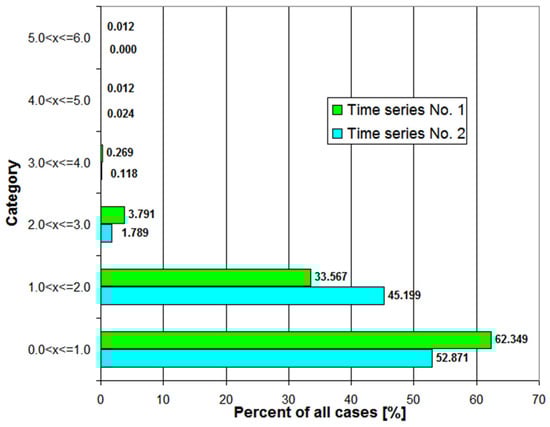
Figure 1.
Percentage distribution of cases in both time series depending on the power demand value.
Figure 2 shows the two daily time series of power demand for the December day considered here. Dynamic changes (rapid jumps) in power demand are clearly visible. For both time series, periods of different length with very similar power demand are characteristic. These periods are usually alternated by much shorter periods (or isolated periods) of much bigger power demand. Meanwhile, Figure 3 shows a specific part of the December day for both time series (from 8:00 to 8:30 a.m.).
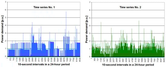
Figure 2.
The two daily time series of power demand for the analyzed December day (figure of time series No. 1 is similar to the one from [44]).
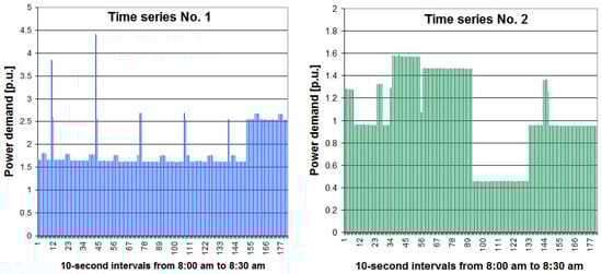
Figure 3.
Two selected 30 min periods of power demand in the considered December day.
The seasonality problem of the time series of power demand was not analyzed due to unavailability of data. For both time series, it was examined whether there were daily variations in power demand in 1 h periods (see Figure 4). For each hour, average 10 s power demand was calculated. For the first time series, R2 equal to 0.3588 was obtained for the function of polynomial degree 8. For the second time series, R2 equal to 0.7464 was obtained for the function of polynomial degree 8. The value of the determination coefficient is low for the first time series and high for the second one. The function of polynomial degree 8 explains about 75% of the variability of the explanatory variable for the second time series. The value of Pearson linear correlation coefficients between the first time series and the second time series of average power demand in 1 h periods calculated based on the functions of polynomial degree 8 is 0.2956 (statistically significant at the 5% significance level).
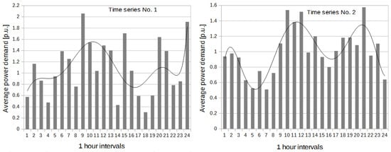
Figure 4.
Daily variation of power demand in 1 h periods for both time series.
For the first time series, the autocorrelation coefficient dynamically decreases from 0.946 (1 period back) to 0.300 (90 periods back, i.e., 15 min) (see Figure 5). The autocorrelation coefficient temporarily increases (a big peak) up to 0.439 (150 periods back, i.e., 25 min). After 240 periods back (40 min), the autocorrelation coefficient falls to almost zero.
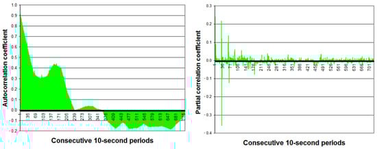
Figure 5.
Autocorrelation function (ACF) and partial autocorrelation function (PACF) of the first time series in the analyzed December day (they are similar to figures of the ACF and PACF from [44]).
For the second time series, the autocorrelation coefficient dynamically decreases from 0.910 (1 period back) to 0.169 (90 periods back, i.e., 15 min) (see Figure 6). Unlike in the first time series, there are also temporary, repeated increases in the autocorrelation coefficient (big peaks) every 180 periods (i.e., 30 min) for the second time series. Autocorrelation coefficient for the first peak is 0.400. The next peaks gradually decrease. It means that the process element of the sewage treatment plant (second time series) probably has a 30 min periodicity.
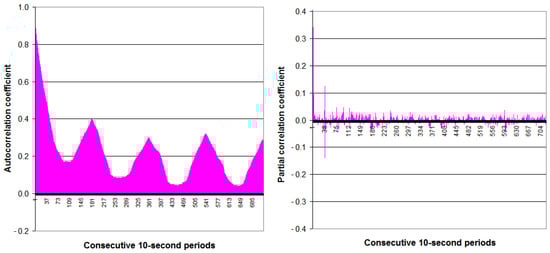
Figure 6.
Autocorrelation function (ACF) and partial autocorrelation function (PACF) of the second time series in the analyzed December day.
For both time series, the partial autocorrelation coefficients are statistically significant (5% significance level) only for the first several values and several single values distant from each other (see Figure 5 and Figure 6).
The Table 2 shows, for both time series, Pearson linear correlation coefficients between 10 s power demand and the potential explanatory variables considered. All correlation coefficients are statistically significant (5% level of significance). For the variable coded AVEW (weighted average), optimal weights were calculated by optimization process using the Newton optimization algorithm which maximized the value of the correlation coefficient between the values of the AVEW and the time series. The sum of weights is equal to 1 (the limit for weights).
Table 2.
Values of Pearson linear correlation coefficients between 10-second power demand of the first time series and the second time series and the explanatory variables considered (partially based on [44]).
It is noteworthy that the sum of the power demand values from period t − 1 with weight w1 and period t − 2 with weight w2 (AVEW) has the maximum correlation coefficient of all potential explanatory variables for both time series. Moreover, the 24-h profile of the variation of power demand (FUNC) seems to be definitely a much better explanatory variable than the hour of power demand (HOUR).
2.2. Analysis of Potential Input Data for Forecasting Methods
Only time-lagged variables are used for the explained variable for methods based on the time series. The selection of explanatory variables is very often related to the process of testing the quality of models.
In the case of other methods using also exogenous variables, the process of selection of adequate explanatory variables can be supported by various methods of selection. Theoretically, for methods other than those based on time series, the forecasting model may contain 1 to 13 explanatory variables (see Table 2). Finding the optimal set of input variables for each model involves checking 8192 (213) different combinations of variables (brute force method). Six methods of selection were used to select proper explanatory variables (see Figure 7).
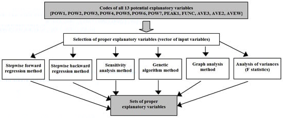
Figure 7.
Scheme of selecting proper sets of explanatory variables.
The purpose of using these methods was to obtain a reduced set of explanatory variables without losing important information for the model and to eliminate non-essential explanatory variables from the model. The results of the selection of explanatory variables are only suggestions for the expert (see Table 3 and Table 4). The expert makes the final decision on the selection of proper explanatory variables by testing forecasting models with various sets of explanatory variables.
Table 3.
Results of initial selection of explanatory variables for all 6 methods of selection—selection for time series No. 1.
Table 4.
Results of the initial selection of explanatory variables for all 6 methods of selection—selection for time series No. 2.
The analysis of the selection of input variables has shown that for both time series (No. 1 and No. 2) the input variable coded HOUR is the input variable most often selected for elimination. Therefore, the input variable coded HOUR has been eliminated from the forecasting process. The most often indicated input variables are coded AVEW (seven indications), AVE3, AVE2 and POW1 (six indications). For time series No. 1, the input variable coded PEAK1 also yielded six indications.
3. Forecasting Methods
This section describes the methods employed in this paper. Forecasts are made using single methods based only on the time series, the other single methods using also additional exogenous variables, including machine learning methods and the most advanced (complex) ensemble methods.
Autoregressive Integrated Moving Average. The autoregressive (AR) part of Autoregressive Integrated Moving Average (ARIMA) indicates that the evolving variable of interest is regressed on its own lagged values. The moving average (MA) part indicates that the regression error is actually a linear combination of error terms whose values occurred contemporaneously and at various times in the past. The term I (integrated) indicates that the data values have been replaced with the difference between their values and the previous values. The model has three parameters for tuning: p is the order (number of time lags) of the autoregressive model, d is the degree of differencing (the number of times the data have had past values subtracted) if the time series is not stationary, and q is the order of the moving-average model. The model is fitted using the least squares approach [45,46].
Autoregressive model. This is a simplified model of ARIMA. There is only one parameter for tuning—p which is the number of time lags. The model with p = 1 is only used for research, assuming that this model is a quality reference model for other methods. The model is fitted using the least squares approach [47,48].
Multiple Linear Regression model. This is a linear model that assumes a linear relationship between input variables (more than one) and the single output variable. The input data are chosen values of lags of the forecasted output variable and other input explanatory variables corelated to the output variable. The model is fitted using the least squares approach [49].
K-Nearest Neighbors. The k-nearest neighbors algorithm is a non-parametric method used for classification and regression [49]. The input consists of k closest training examples in the feature space. In k-nearest neighbors (KNN) regression, the property value for the object is the output. This value is the average of the values of k nearest neighbors. The main hyperparameter for tuning is the number of nearest neighbors. Distance metric is the second hyperparameter.
Support Vector Regression. Support vector machine (SVM) for regression of the Gaussian kernel (non-linear regression) transforms the classification task into regression by defining a certain tolerance region with the width of ε around the target [49,50]. The learning task is reduced to the quadratic optimization problem and dependents on several hyperparameters: regularization constant C, width parameter σ of the Gaussian kernel, and tolerance ε.
Type MLP artificial neural network. This is a class of feedforward artificial neural networks (ANNs). MLP is a popular and effective non-linear or linear (depending on the type of activation function in hidden layer/layers and output layer) global approximator [51,52]. It consists of one input layer, typically has one or two hidden layers, one output layer and often uses the backpropagation algorithm for supervised learning. The main hyperparameter for tuning is the number of neurons in hidden layer(s). The Broyden–Fletcher–Goldfarb–Shanno (BFGS) method used for solving unconstrained non-linear optimization problems has been chosen as a learning algorithm of the neural network.
Interval Type-2 Fuzzy Logic System. Type-2 fuzzy logic systems (T2 FLSs) use type-2 fuzzy sets (T2 FS). Type-2 fuzzy sets were defined by L. Zadeh in 1975 as an extension of type-1 fuzzy sets (T1 FS). Further works on the subject were carried out by Karnik, Mendel and Liang [53,54,55]. T2 FSs are characterized by 3-dimensional membership functions (MF), which include footprint of uncertainty (FOU) [56]. The FOU and the third dimension of MF deliver additional degrees of freedom, which enables them to deal with uncertainties. The structure of type-2 fuzzy logic inference system is presented in Figure 8. The following components of T2 FLSs can be distinguished: fuzzification block, fuzzy inference block, base of fuzzy rules, type reduction block, and defuzzification block. The conversion of T2 FS to T1 FS takes place in the type reduction block. The Karnik–Mendel (KM) algorithm is usually applied for type reduction [54].
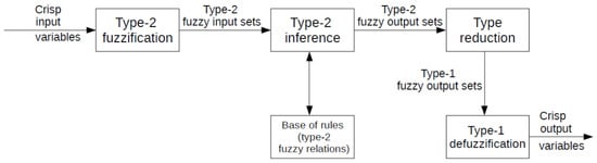
Figure 8.
The structure of type-2 fuzzy logic inference system; elaborated based on [56].
Taking into account computational complexity of T2 FLSs, interval type-2 fuzzy logic systems (IT2FLSs) (see, e.g., [56]) are often used in practice [57]. The latter systems are characterized by a smaller computational effort of inference process in comparison with T2 FLSs. The IT2FLS with Takagi–Sugeno–Kang inference model, i.e., the IT2 TSK FLS [56], or the IT2FLS with Sugeno inference model, i.e., the IT2 S FLS, can be distinguished among the different IT2FLSs. The latter systems require a lower number of model parameters and in this way, they seem to be easier to use. In the training process of the system being designed to determine values of its particular parameters, genetic algorithm (GA) or PSO algorithm can be used.
Ensemble methods, using more than one individual predictor and supported by a simple or more complex integration system of individual forecasts, are addressed next. The general scheme of establishing an ensemble of predictors is presented in Figure 9. The simplest integration system is weighted averaging of individual predictors. The most advanced integrator systems are based on machine learning methods.
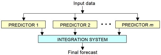
Figure 9.
General structure of ensemble methods.
Random Forest Regression. Random forest is an ensemble method based on many single decision trees. Random forest is a versatile machine learning algorithm that can perform both classification and regression tasks. In the regression task, the prediction in a single decision tree is the average target value of all instances associated with the single leaf node. The final prediction is the average value of all m single decision trees. The regularization hyperparameters depend on the algorithm used, but generally restricted are: the maximum depth of the single decision tree, maximum number of levels in each decision tree, minimum number of data points placed in a node before the node is split, minimum number of data points allowed in a leaf node and maximum number of nodes. The number of predictors for each of the m single decision trees is made by the random choice of k predictors from all available n predictors [49,58,59].
Gradient Boosted Trees for Regression. Gradient boosting refers to an ensemble method that can combine several weak learners into a strong learner. It works by sequentially adding predictors (single decision tree) to the ensemble, each one correcting its predecessor. The method tries to fit the new predictor to the residual errors made by the previous predictor. The final prediction is the average value from all m single decision trees. This machine learning method is very effective and is recommended in many papers for forecasting tasks [22,60,61]. In comparison with random forest, this method has one additional hyperparameter—learning rate which scales the contribution of each tree [49,59,62,63].
Weighted Averaging Ensemble. This is an integration of the results of selected predictors into final verdict of the ensemble. The final forecast is defined as the average of the results produced by all m predictors organized in an ensemble [50]. The final prediction result is calculated by formula (1). This formula makes use of the stochastic distribution of the predictive errors. The process of averaging reduces the final error of forecasting.
where, i is the prediction point, is the final predicted value, is predicted value by predictor number j, and m is the number of predictors in ensemble. Note: all weights are equal in this case.
The averaging of the forecast results is an established method of reducing the variance of forecast errors. An important condition for including the predictor into the ensemble is independent operation from the others and also similar level of prediction error [50]. Two main strategies of predictor choice were tested:
- The choice of predictors based on RMSE (code WAE_RMSE). Three or four predictors based on the smallest RMSE errors on validation subset and only predictors of different types are selected to the ensemble;
- The choice of predictors based on RMSE and R (code WAE_R/RMSE). The time series of the residues from forecasts should be most different from each other and RMSE error should be small. The choice algorithm of predictors based on RMSE and R is presented in Figure 10.
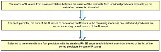 Figure 10. Algorithm of selection of predictors to the ensemble based on RMSE and R.
Machine Learning (ML) as an Integrator of Ensemble. This is an integration of the results of the selected predictors into final verdict of the ensemble using ML model. Four predictors based on the smallest RMSE errors on validation subset are included in the ensemble, and these predictors must be of different types. Four ML methods are adopted as the integrator of the ensemble: MLP, KNN, random forest (RF) and linear regression (LR). Each ML integrator uses forecasts of power demand from four individual predictors as input data and the real values of power demand as the output. A training dataset is used for training ML integrator, and a validation dataset is used for RMSE control and tuning of hyperparameters. Finally, the evaluation criteria are verified against the test dataset. The general structure of four machine learning methods as an integrator of ensemble is presented in Figure 11 [49,64].
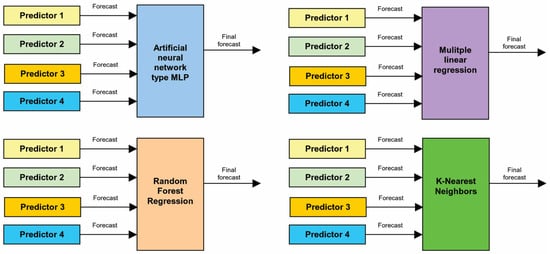
Figure 11.
The general structure of four machine learning methods as an integrator of ensemble.
Summary description of fifteen tested forecasting methods is shown in Table 5. There are two methods based on time series and thirteen methods based on time series and exogenous input data. The eight methods are ensemble methods, and the seven ones are single methods. Ten methods all are machine learning methods.
Table 5.
Summary description of fifteen tested forecasting methods.
4. Evaluation Criteria
In order to have a broader view of the quality of individual forecasting models, seven evaluation criteria are used. The main evaluation criterion is Root Mean Square Error (RMSE) due to the specificity of the forecast time series (more important for predictions of values which are greater than values close to zero or very small). Other major evaluation criteria are Maximum Absolute Error (MAE), Symmetric Mean Absolute Percentage Error (sMAPE) and Mean Absolute Percentage Error (MAPE) errors. Three auxiliary evaluation criteria are R (Pearson linear correlation coefficient), Mean Bias Error (MBE) and Maximum Absolute Error (MaxAE).
Root Mean Square Error is calculated by formula (2). RMSE is sensitive to large errors and is more useful when large errors are particularly undesirable.
where, is the predicted value, is the actual value, and is the number of prediction points.
Mean Absolute Error is calculated by formula (3)
In the process of forecasting of electric power demand, changes in RMSE and MAE have the same trend, and the smaller the two error values, the more accurate the prediction results.
Maximum Absolute Error is calculated by formula (4)
Mean Absolute Percentage Error is calculated by formula (5). MAPE is asymmetric and it puts a heavier penalty on negative errors (when forecasts are higher than actuals) than on positive errors. This is due to the fact that percentage error cannot exceed 100% for forecasts that are too low. Meanwhile, there is no upper limit for forecasts which are too high. As a result, MAPE will favor models that yield under-forecast rather than over-forecast.
Symmetric Mean Absolute Percentage Error is calculated by formula (6). sMAPE error overcomes the asymmetry of MAPE error— the boundlessness of the forecasts that are higher than the actuals and it has both the lower (0%) and the upper (200%) bounds.
Mean Bias Error captures the average bias in the prediction and is calculated by formula (7)
Pearson linear correlation coefficient of the observed and predicted data is calculated by formula (8)
where, is the covariance value between the actually observed and predicted data, and denotes standard deviation of the appropriate variable.
The bigger the error R value (range from −1 to 1), the more accurate the prediction results.
5. Results
This section presents an extensive comparative analysis of very short-term forecasting methods for active power demand in two different technological elements of the sewage treatment plant.
Both time series, including 8640 periods of 10 s, were divided into three subsets—training and validation subsets were composed of the initial 85% of time series (division into training and validation subsets which are different depending on the forecasting method) and the test subset comprised the last 15% of the time series. The training subset is used for estimation of model parameters. The validation subset is used for tuning hyperparameters of parts of methods. The test subset is applied to the final results of errors of the applied methods. For most of the methods, a random strategy choice of data for training and validation subsets was applied to get the right representation of data in each subset. Some methods, e.g., gradient boosted trees (GBT), used bootstrap technique for the choice of the training and validation subsets from the initial 85% data of the time series. Some other methods, e.g., AR, used only the training subset (the initial 85% of data in the time series) without validation subset.
Table 6 shows performance measures of proposed single methods (on test subset) for time series No. 1. Detailed description of the results of hyperparameters tuning for the single methods tested is provided in Table A1 of Appendix A.
Table 6.
Performance measures of proposed single methods (on test subset) for time series No. 1.
Table 7 presents performance measures of proposed ensemble methods (on test subset) for time series No. 1. Detailed description of the results of hyperparameters tuning for the ensemble methods tested is provided in Table A2 of Appendix A.
Table 7.
Performance measures of proposed ensemble methods (on test subset) for time series No. 1.
Table 8 shows performance measures of proposed single methods (on test subset) for time series No. 2. Detailed description of the results of hyperparameters tuning for the single methods tested is provided in Table A3 of Appendix A.
Table 8.
Performance measures of proposed single methods (on test subset range) for time series No. 2.
Table 9 presents performance measures of proposed ensemble methods (on test subset) for time series No. 2. Detailed description of the results of hyperparameters tuning for the ensemble methods tested is provided in Table A4 of Appendix A.
Table 9.
Performance measures of proposed ensemble methods (on test subset) for time series No. 2.
6. Discussion
This section discusses the forecasts obtained for active power demand in two different technological parts of a sewage treatment plant.
Based on the results from Table 6, the following preliminary conclusions can be drawn regarding the proposed single methods for time series No. 1:
- The best methods in terms of RMSE value are, respectively: MLP, LR, ARIMA; for MLP and LR, a more favorable solution is to utilize all 11 input data instead of 5 input data selected on the basis of the analysis of variables selection;
- An advantage of the LR method in comparison with MLP is very short time of calculations, low computational complexity and no necessity of proper selection of hyperparameter values which are required by MLP (only selection of the most advantageous input data may be needed);
- Qualitative differences between the best three methods are very small;
- The worst methods in terms of RMSE value, in comparison with the reference method AR(1), are: SVR, KNN and IT2FLS; for IT2FLS method the use of five input data instead of four last time-lagged values of variables of time series being forecast allowed to decrease RMSE error;
- A disadvantage of IT2FLS is very long time of calculations (the time depends on CPU and RAM memory of computer being used) and the necessity of proper selection of many hyperparameter values; for the KNN method with five input data, the smallest MAPE and sMAPE errors have been obtained from all tested methods, although the RMSE error for the method is significant in comparison with the best methods.
In turn, based on the results from Table 7, it is possible to formulate the following preliminary conclusions concerning the proposed ensemble methods for time series No. 1:
- The best ensemble methods are, respectively: GBT and LR as an integrator of ensemble; for GBT, it is more useful to utilize all 11 input data;
- GBT ensemble method seems to be more useful than LR as an integrator of ensemble, considering greater simplicity of the method (no necessity to integrate four different method types), in which the ensemble is an internal component of the algorithm (single decision trees);
- All ensemble methods have smaller RMSE errors than the reference AR(1) method;
- Among ensemble methods, only RF as an integrator of ensemble has greater RMSE error than the best single method, i.e., MLP; it clearly shows that using ensemble methods (except RF) is justified in this forecasting exercise and allows us to decrease RMSE error in comparison with single methods;
- Similarly, as in the KNN single method, using KNN as an integrator of ensemble allows us to get the smallest MAPE and sMAPE errors of all tested ensemble methods, at the same time the RMSE error for the method is significant in comparison with the best ensemble methods;
- WAE_R/RMSE ensemble method is less advantageous than WAE_RMSE ensemble method;
- RF is the worst of all ensemble methods.
Based on the results from Table 8, the following preliminary conclusions can be drawn which concern the proposed single methods for time series No. 2:
- The best methods in terms of RMSE value are, respectively: LR, ARIMA and MLP; for MLP and for LR, it is more useful to utilize 5 input data, selected on the basis of the analysis of variables selection, instead of all 11 input data;
- Qualitative differences among the best three methods are very small;
- The worst methods in terms of RMSE value, in comparison with the reference method AR(1), are: KNN utilizing 11 input data and IT2FLS; for IT2FLS, the use of five input data instead of four last time-lagged values of variables of time series being forecast allowed us to decrease RMSE error.
Lastly, based on the results from Table 9, the following partial conclusions can be formulated concerning proposed ensemble methods for time series No. 2:
- The best ensemble methods are: MLP, GBT and LR as an integrator of ensemble; for GBT, it is more useful to utilize all 11 input data;
- GBT ensemble method seems to be more useful than MLP as an integrator of ensemble because of the greater simplicity of the method (no necessity to integrate four different method types), in which the ensemble is an internal algorithm component (single decision trees);
- All ensemble methods have smaller RMSE errors than the reference method AR(1);
- Among ensemble methods, only the last four ones in the ranking (as integrators of ensemble) have a greater RMSE error than the best single method, i.e., LR(6); it suggests that using an ensemble method (except for the last four ones) is justified in this forecasting exercise and allows us to decrease RMSE error in comparison with single methods;
- As for the KNN single method, using KNN as an integrator of ensemble resulted in the smallest MAPE and sMAPE errors of all tested ensemble methods, at the same time the RMSE error for the method is significant in comparison with the best ensemble methods;
- WAE_RMSE ensemble method is more useful than WAE_R/RMSE ensemble method;
- RF is the worst of all ensemble methods.
Table 10 shows the best eight methods chosen from single and ensembles methods for both time series sorted in descending order by RMSE and the basic (reference) method.
Table 10.
Summary comparison—the best eight methods chosen from single and ensembles methods for both time series sorted in descending order by RMSE and the basic (reference) method.
Actual values from test range (subset) of time series and the forecasted values by the best method are presented in Figure 12 for time series No. 1 and in Figure 13 for time series No. 2.
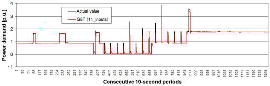
Figure 12.
Actual values from the test range (subset) of time series No. 1 and the forecast values by the best method.
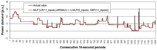
Figure 13.
Actual values from the test range (subset) of time series No. 2 and the forecast values by the best method.
7. Conclusions
Very dynamic random rises of power demand of only 10 s duration (basic time interval) have been a major problem, and are impossible to forecast very accurately in practice. It is difficult to identify the best of the single methods. However, for both time series, the following three methods have always performed best: MLP, LR and ARIMA. Finally, from the point of view of forecasting efficiency (RMSE error value) and complexity level of the method, the most beneficial method is the GBT ensemble method, which utilizes all 11 input data. Comparative analysis of the results obtained for both time series shows that single methods—KNN, IT2FLS (with the use of four last time-lagged values of variables of time series being forecasted) and SVR—belong to the category of less recommended methods for this type of forecasting exercise.
Other observations and conclusions of the study can be summarized as follows:
- (1)
- The fact that the two time series being forecast are untypical ones means that achieving significantly smaller RMSE errors than in the case of the reference method AR(1) is difficult, but the studies carried out show that it is possible. For time series No. 1, improvement in comparison with the AR(1) method is equal to 10.94%, whereas for time series No. 2, improvement reaches 19.00% for the best methods being tested.
- (2)
- For both time series, the validity of using a vast majority of ensemble methods in comparison with single methods has been demonstrated. It is necessary to pay attention to the great complexity of such methods, their time demand as well as very small differences in RMSE error value for the best eight ensemble methods for both forecast time series.
- (3)
- RF is the worst performing ensemble method in both time series, thus this technique of machine learning should not be preferred as an ensemble method for this forecasting exercise.
- (4)
- Very small MAPE and sMAPE errors for the KNN method, used as a single method or applied as an integrator of ensemble, together with quite large RMSE error at the same time, is a characteristic and recurring phenomenon.
- (5)
- The impact of proper selection of input data varies from case to case; some methods achieved smaller RMSE errors with the use of 5 input data, whereas other methods performed better with the use of 11 input data, depending on time series being forecast, the exception being the GBT method, for which it was more useful to utilize all 11 input data.
- (6)
- For both time series, it was better to use the criterion of the least RMSE errors for selection of the four most beneficial predictors used for constructing the ensemble methods, as well as the rule of dissimilarity of predictor action, rather than to use an additional criterion of the biggest differences in rests from forecasts obtained with the use of methods being candidates to the ensemble.
The studies conducted allow us to conclude that there are effective methods of forecasting very short-term (10 s) power demand values (characterized by big dynamics of load changes) which are suitable for practical use, although it is a very complicated forecasting exercise. This is due to very dynamic random rises of the received power of 10 s duration. In further studies on methods of very short-term forecasting of power demand, we intend to conduct, among others, research on the development of forecasts for time intervals from t + 1 to t + 6, that is, with the time horizon up to 1 min.
Author Contributions
Conceptualization, P.P. and M.P. (Mirosław Parol); formal analysis, P.P.; methodology, P.P., P.K. and M.P. (Mirosław Parol); investigation, P.P., P.K. and M.P. (Mariusz Piotrowski); supervision, M.P. (Mirosław Parol); validation, P.P.; writing, P.P., M.P. (Mirosław Parol), P.K. and M.P. (Mariusz Piotrowski); visualization P.P.; project administration, P.P. All authors have read and agreed to the published version of the manuscript.
Funding
This research received no external funding.
Acknowledgments
The dataset used for calculations in this paper has been collected under the RIGRID research project being part of the ERA-Net Smart Grid Plus initiative, having a support from the European Union’s Horizon 2020 research and innovation program. The data acquisition system used for the mentioned data measurements has been also developed under the RIGRID project.
Conflicts of Interest
The authors declare no conflict of interest.
Abbreviation
The following abbreviations are used in this manuscript:
| ACF | Autocorrelation Function |
| APN AE | Access Point Name Absolute Error |
| EIASC | Enhanced iterative algorithm with stop condition |
| ANN | Artificial Neural Network |
| AR | Autoregressive model |
| ARIMA | Autoregressive Integrated Moving Average |
| BFGS | Broyden–Fletcher–Goldfarb–Shanno algorithm |
| EKM | Enhanced Karnik–Mendel |
| FLS | Fuzzy Logic System |
| GA | Genetic Algorithm |
| GBT | Gradient Boosted Trees |
| IASC | Iterative algorithm with stop condition |
| IT2FLS | Interval Type-2 Fuzzy Logic System |
| KM | Karnik–Mendel |
| KNN | K-Nearest Neighbors |
| MAE | Mean Absolute Error |
| MAPE | Mean Absolute Percentage Error |
| MBE | Mean Bias Error |
| ML MLP | Machine Learning Multi-Layer Perceptron |
| MaxAE | Maximum Absolute Error |
| LR | Linear Regression |
| PACF | Partial Autocorrelation Function |
| PSO | Particle Swarm Optimization |
| R | Pearson linear correlation coefficient |
| R2 | Determination coefficient |
| RBF | Radial Base Function |
| RF | Random Forest |
| RMSE | Root Mean Square Error |
| sMAPE | Symmetric Mean Absolute Percentage Error |
| SVM | Support Vector Machine |
| SVR | Support Vector Regression |
Appendix A
Table A1 shows the results of hyperparameter tuning for proposed single methods for time series No. 1.
Table A1.
Results of hyperparameter tuning for proposed single methods for time series No. 1.
Table A2 presents the results of hyperparameter tuning for the proposed ensemble methods for time series No. 1.
Table A2.
Results of hyperparameter tuning for the proposed ensemble methods for time series No. 1.
Table A3 shows the results of hyperparameter tuning for proposed single methods for time series No. 2.
Table A3.
Results of hyperparameters tuning for proposed single methods for time series No. 2.
Table A4 presents the results of hyperparameter tuning for the proposed ensemble methods for time series No. 2.
Table A4.
Results of hyperparameter tuning for the proposed ensemble methods for time series No. 2.
References
- Microgrids 1: Engineering, Economics, & Experience—Capabilities, Benefits, Business Opportunities, and Examples—Microgrids Evolution Roadmap; Study Committee: C6, CIGRÉ Working Group C6.22, Technical Brochure 635; CIGRE: Paris, France, 2015.
- Marnay, C.; Chatzivasileiadis, S.; Abbey, C.; Iravani, R.; Joos, G.; Lombardi, P.; Mancarella, P.; von Appen, J. Microgrid evolution roadmap. Engineering, economics, and experience. In Proceedings of the 2015 Int. Symp. on Smart Electric Distribution Sys-tems and Technologies (EDST15); CIGRE SC C6 Colloquium, Vienna, Austria, 8–11 September 2015. [Google Scholar]
- Hatziargyriou, N.D. (Ed.) Microgrids: Architectures and Control; Wiley-IEEE Press: Hoboken, NJ, USA, 2014. [Google Scholar]
- Low Voltage Microgrids. Joint Publication Edited by Mirosław Parol; Publishing House of the Warsaw University of Technology: Warsaw, Poland, 2013. (In Polish)
- Li, Y.; Nejabatkhah, F. Overview of control, integration and energy management of microgrids. J. Mod. Power Syst. Clean Energy 2014, 2, 212–222. [Google Scholar] [CrossRef]
- Olivares, D.E.; Canizares, C.A.; Kazerani, M. A Centralized Energy Management System for Isolated Microgrids. IEEE Trans. Smart Grid 2014, 5, 1864–1875. [Google Scholar] [CrossRef]
- Han, Y.; Zhang, K.; Li, H.; Coelho, E.A.A.; Guerrero, J.M. MAS-Based Distributed Coordinated Control and Optimization in Microgrid and Microgrid Clusters: A Comprehensive Overview. IEEE Trans. Power Electron. 2018, 33, 6488–6508. [Google Scholar] [CrossRef]
- Morstyn, T.; Hredzak, B.; Agelidis, V.G. Control strategies for microgrids with distributed energy storage systems: An over-view. IEEE Trans. Smart Grid 2018, 9, 3652–3666. [Google Scholar] [CrossRef]
- Li, Q.; Peng, C.; Chen, M.; Chen, F.; Kang, W.; Guerrero, J.M.; Abbott, D. Networked and Distributed Control Method With Optimal Power Dispatch for Islanded Microgrids. IEEE Trans. Ind. Electron. 2016, 64, 493–504. [Google Scholar] [CrossRef]
- Parol, R.; Parol, M.; Rokicki, Ł. Implementation issues concerning optimal operation control algorithms in low voltage mi-crogrids. In Proceedings of the 5th Int. Symp. on Electrical and Electronics Engineering (ISEEE-2017), Galati, Romania, 20–22 October 2017; pp. 1–7. [Google Scholar]
- Lopes, J.A.P.; Moreira, C.L.; Madureira, A.G. Defining Control Strategies for MicroGrids Islanded Operation. IEEE Trans. Power Syst. 2006, 21, 916–924. [Google Scholar] [CrossRef]
- Zhao, H.; Wu, Q.; Wang, C.; Cheng, L.; Rasmussen, C.N. Fuzzy logic based coordinated control of battery energy storage system and dispatchable distributed generation for microgrid. J. Mod. Power Syst. Clean Energy 2015, 3, 422–428. [Google Scholar] [CrossRef]
- Parol, M.; Rokicki, Ł.; Parol, R. Towards optimal operation control in rural low voltage microgrids. Bull. Pol. Ac. Tech. 2019, 67, 799–812. [Google Scholar]
- Parol, M.; Kapler, P.; Marzecki, J.; Parol, R.; Połecki, M.; Rokicki, Ł. Effective approach to distributed optimal operation con-trol in rural low voltage microgrids. Bull. Pol. Ac. Tech. 2020, 68, 661–678. [Google Scholar]
- Niu, D.; Pu, D.; Dai, S. Ultra-Short-Term Wind-Power Forecasting Based on the Weighted Random Forest Optimized by the Niche Immune Lion Algorithm. Energies 2018, 11, 1098. [Google Scholar] [CrossRef]
- Bokde, N.; Feijóo, A.; Villanueva, D.; Kulat, K. A Review on Hybrid Empirical Mode Decomposition Models for Wind Speed and Wind Power Prediction. Energies 2019, 12, 254. [Google Scholar] [CrossRef]
- Adnan, R.M.; Liang, Z.; Yuan, X.; Kisi, O.; Akhlaq, M.; Li, B. Comparison of LSSVR, M5RT, NF-GP, and NF-SC Models for Predictions of Hourly Wind Speed and Wind Power Based on Cross-Validation. Energies 2019, 12, 329. [Google Scholar] [CrossRef]
- Würth, I.; Valldecabres, L.; Simon, E.; Möhrlen, C.; Uzunoğlu, B.; Gilbert, C.; Giebel, G.; Schlipf, D.; Kaifel, A. Minute-Scale Forecasting of Wind Power—Results from the Collaborative Workshop of IEA Wind Task 32 and 36. Energies 2019, 12, 712. [Google Scholar] [CrossRef]
- Liu, F.; Li, R.; Dreglea, A. Wind Speed and Power Ultra Short-Term Robust Forecasting Based on Takagi–Sugeno Fuzzy Model. Energies 2019, 12, 3551. [Google Scholar] [CrossRef]
- Sun, S.; Fu, J.; Li, A. A Compound Wind Power Forecasting Strategy Based on Clustering, Two-Stage Decomposition, Parameter Optimization, and Optimal Combination of Multiple Machine Learning Approaches. Energies 2019, 12, 3586. [Google Scholar] [CrossRef]
- Son, N.; Yang, S.; Na, J. Hybrid Forecasting Model for Short-Term Wind Power Prediction Using Modified Long Short-Term Memory. Energies 2019, 12, 3901. [Google Scholar] [CrossRef]
- Zheng, H.; Wu, Y. A XGBoost Model with Weather Similarity Analysis and Feature Engineering for Short-Term Wind Power Forecasting. Appl. Sci. 2019, 9, 3019. [Google Scholar] [CrossRef]
- Mujeeb, S.; Alghamdi, T.A.; Ullah, S.; Fatima, A.; Javaid, N.; Saba, T. Exploiting Deep Learning for Wind Power Forecasting Based on Big Data Analytics. Appl. Sci. 2019, 9, 4417. [Google Scholar] [CrossRef]
- Wang, K.; Niu, D.; Sun, L.; Zhen, H.; Liu, J.; De, G.; Xu, X. Wind Power Short-Term Forecasting Hybrid Model Based on CEEMD-SE Method. Process. 2019, 7, 843. [Google Scholar] [CrossRef]
- Valldecabres, L.; Nygaard, N.G.; Vera-Tudela, L.; von Bremen, L.; Kühn, M. On the Use of Dual-Doppler Radar Measurements for Very Short-Term Wind Power Forecasts. Remote Sens. 2018, 10, 1701. [Google Scholar] [CrossRef]
- Zhao, H.; Zhao, H.; Guo, S. Short-Term Wind Electric Power Forecasting Using a Novel Multi-Stage Intelligent Algorithm. Sustainability 2018, 10, 881. [Google Scholar] [CrossRef]
- Zhou, J.; Yu, X.; Jin, B. Short-Term Wind Power Forecasting: A New Hybrid Model Combined Extreme-Point Symmetric Mode Decomposition, Extreme Learning Machine and Particle Swarm Optimization. Sustainability 2018, 10, 3202. [Google Scholar] [CrossRef]
- Fu, C.; Li, G.Q.; Lin, K.P.; Zhang, H.J. Short-Term Wind Power Prediction Based on Improved Chicken Algorithm Optimiza-tion Support Vector Machine. Sustainability 2019, 11, 512. [Google Scholar] [CrossRef]
- Meng, X.; Wang, R.; Zhang, X.; Wang, M.; Ma, H.; Wang, Z. Hybrid Neural Network Based on GRU with Uncertain Factors for Forecasting Ultra-short-term Wind Power. In Proceedings of the 2020 2nd International Conference on Industrial Artificial Intelligence (IAI), Shenyang, China, 23–25 October 2020. [Google Scholar]
- Carpinone, A.; Giorgio, M.; Langella, R.; Testa, A. Markov chain modeling for very-short-term wind power forecasting. Electr. Power Syst. Res. 2015, 122, 152–158. [Google Scholar] [CrossRef]
- Tato, J.H.; Brito, M.C. Using Smart Persistence and Random Forests to Predict Photovoltaic Energy Production. Energies 2018, 12, 100. [Google Scholar] [CrossRef]
- Zhu, R.; Guo, W.; Gong, X. Short-Term Photovoltaic Power Output Prediction Based on k-Fold Cross-Validation and an En-semble Model. Energies 2019, 12, 1220. [Google Scholar]
- Xie, T.; Zhang, G.; Liu, H.; Liu, F.; Du, P. A Hybrid Forecasting Method for Solar Output Power Based on Variational Mode Decomposition, Deep Belief Networks and Auto-Regressive Moving Average. Appl. Sci. 2018, 8, 1901. [Google Scholar] [CrossRef]
- Abdullah, N.A.; Rahim, N.A.; Gan, C.K.; Adzman, N.N. Forecasting Solar Power Using Hybrid Firefly and Particle Swarm Optimization (HFPSO) for Optimizing the Parameters in a Wavelet Transform-Adaptive Neuro Fuzzy Inference System (WT-ANFIS). Appl. Sci. 2019, 9, 3214. [Google Scholar] [CrossRef]
- Nespoli, A.; Mussetta, M.; Ogliari, E.; Leva, S.; Fernández-Ramírez, L.; García-Triviño, P. Robust 24 Hours ahead Forecast in a Microgrid: A Real Case Study. Electronics 2019, 8, 1434. [Google Scholar] [CrossRef]
- Huang, J.; Boland, J. Performance Analysis for One-Step-Ahead Forecasting of Hybrid Solar and Wind Energy on Short Time Scales. Energies 2018, 11, 1119. [Google Scholar] [CrossRef]
- Dudek, G. Short-Term Load Forecasting Using Random Forests. In Intelligent Systems’2014. Advances in Intelligent Systems and Computing; Filev, D., Ed.; Springer: Berlin/Heidelberg, Germany, 2015; Volume 323, pp. 821–828. [Google Scholar]
- Kim, C.; Yu, I.; Song, Y.H. Kohonen neural network and wavelet transform based approach to short-term load fore-casting. Electr. Power Syst. Res. 2002, 63, 169–176. [Google Scholar] [CrossRef]
- Dudek, G. Pattern-based local linear regression models for short-term load forecasting. Electr. Power Syst. Res. 2016, 130, 139–147. [Google Scholar] [CrossRef]
- Shamsollahi, P.; Cheung, K.W.; Chen, Q.; Germain, E.H. A neural network based very short term load forecaster for the interim ISO New England electricity market system. In Proceedings of the 2001 Power Industry Computer Applications Conf., Sydney, Australia, 20–24 May 2001; pp. 217–222. [Google Scholar]
- Parol, M.; Piotrowski, P. Very short-term load forecasting for optimum control in microgrids. In Proceedings of the 2nd International Youth Conference on Energetics (IYCE 2009), Budapest, Hungary, 4–6 June 2009; pp. 1–6. [Google Scholar]
- Parol, M.; Piotrowski, P. Electrical energy demand forecasting for 15 minutes forward for needs of control in low voltage electrical networks with installed sources of distributed generation. Przegląd Elektrotechniczny (Electr. Rev.) 2010, 86, 303–309. (In Polish) [Google Scholar]
- Hernandez, L.; Baladron, C.; Aguiar, J.M.; Carro, B.; Sanchez-Esguevillas, A.J.; Lloret, J.; Massana, J. A Survey on Electric Power Demand Forecasting: Future Trends in Smart Grids, Microgrids and Smart Buildings. IEEE Commun. Surv. Tutor. 2014, 16, 1460–1495. [Google Scholar] [CrossRef]
- Parol, M.; Piotrowski, P.; Piotrowski, M. Very short-term forecasting of power demand of big dynamics objects. E3S Web Conf. 2019, 84, 01007. [Google Scholar] [CrossRef]
- Ziegel, E.R.; Box, G.; Jenkins, G.; Reinsel, G. Time Series Analysis, Forecasting, and Control. Technometrics 1995, 37, 238. [Google Scholar] [CrossRef]
- Brockwell, P.J.; Davis, R.A. Introduction to Time Series and Forecasting; Springer: Berlin/Heidelberg, Germany, 2016. [Google Scholar]
- Shumway, R.H.; Stoffer, D.S. Time Series Analysis and Its Applications: With R Examples, 4th ed.; Springer: Berlin/Heidelberg, Germany, 2017. [Google Scholar]
- Rojas, I.; Pomares, H.; Valenzuela, O. (Eds.) Time Series Analysis and Forecasting. Selected Contributions from ITISE 2017; Springer: Berlin/Heidelberg, Germany, 2018. [Google Scholar]
- Géron, A. Hands-on Machine Learning with Scikit-Learn, Keras, and TensorFlow, 2nd ed.; O’Reilly Media, Inc.: Sevastopol, CA, USA, 2019. [Google Scholar]
- Osowski, S.; Siwek, K. Local dynamic integration of ensemble in prediction of time series. Bull. Pol. Acad. Tech. 2019, 67, 517–525. [Google Scholar]
- Piotrowski, P.; Baczyński, D.; Kopyt, M.; Szafranek, K.; Helt, P.; Gulczyński, T. Analysis of forecasted meteorological data (NWP) for efficient spatial forecasting of wind power generation. Electr. Power Syst. Res. 2019, 175, 105891. [Google Scholar] [CrossRef]
- Dudek, G. Multilayer perceptron for short-term load forecasting: From global to local approach. Neural Comput. Appl. 2019, 32, 3695–3707. [Google Scholar] [CrossRef]
- Karnik, N.; Mendel, J.; Liang, Q. Type-2 fuzzy logic systems. IEEE Trans. Fuzzy Syst. 1999, 7, 643–658. [Google Scholar] [CrossRef]
- Karnik, N.N.; Mendel, J.M. Centroid of a type-2 fuzzy set. Inf. Sci. 2001, 132, 195–220. [Google Scholar] [CrossRef]
- Mendel, J.; John, R. Type-2 fuzzy sets made simple. IEEE Trans. Fuzzy Syst. 2002, 10, 117–127. [Google Scholar] [CrossRef]
- Khosravi, A.; Nahavandi, S.; Creighton, D.; Srinivasan, D. Interval Type-2 Fuzzy Logic Systems for Load Forecasting: A Comparative Study. IEEE Trans. Power Syst. 2012, 27, 1274–1282. [Google Scholar] [CrossRef]
- Liang, Q.; Mendel, J.M. Interval type-2 fuzzy logic systems: Theory and design. IEEE Trans. Fuzzy Syst. 2000, 8, 535–550. [Google Scholar] [CrossRef]
- Kam, H.T. The Random Subspace Method for Constructing Decision Forests. IEEE Trans. Pattern Anal. 1998, 20, 832–844. [Google Scholar]
- Berk, R.A. Statistical Learning from a Regression Perspective, 3rd ed.; Springer: Berlin/Heidelberg, Germany, 2020. [Google Scholar]
- Abbasi, R.A.; Javaid, N.; Ghuman, M.N.J.; Khan, Z.A.; Ur Rehman, S. Amanullah Short Term Load Forecasting Using XGBoost. In Web, Artificial Intelligence and Network Applications. WAINA 2019. Advances in Intelligent Systems and Computing; Barolli, L., Takizawa, M., Xhafa, F., Enokido, T., Eds.; Springer: Berlin/Heidelberg, Germany, 2019; Volume 927. [Google Scholar]
- Wang, W.; Shi, Y.; Lyu, G.; Deng, W. Electricity Consumption Prediction Using XGBoost Based on Discrete Wavelet Transform. In Proceedings of the 2017 2nd International Conference on Artificial Intelligence and Engineering Applications (AIEA 2017), Guilin, China, 23–24 September 2017; pp. 716–729. [Google Scholar]
- Friedman, J.H. Stochastic gradient boosting. Comput. Stat. Data Anal. 2002, 38, 367–378. [Google Scholar] [CrossRef]
- Hastie, T.; Tibshirani, R.; Friedman, J.H. The elements of Statistical Learning. Data Mining, Inference, and Prediction, 2nd ed.; Springer: Berlin/Heidelberg, Germany, 2009. [Google Scholar]
- Alpaydin, E. Introduction to Machine Learning, 4th ed.; MIT Press: Cambridge, MA, USA, 2020. [Google Scholar]


Publisher’s Note: MDPI stays neutral with regard to jurisdictional claims in published maps and institutional affiliations. |
© 2021 by the authors. Licensee MDPI, Basel, Switzerland. This article is an open access article distributed under the terms and conditions of the Creative Commons Attribution (CC BY) license (http://creativecommons.org/licenses/by/4.0/).