Energy Storage Economic Optimization Scheduling Method for Multi-Scene Demand of Peak and Frequency Modulation

Abstract

Energy storage (ES) only contributes to a single-scene (peak or frequency modulation (FM)) control of the power grid, resulting in low utilization rate and high economic cost. Herein, a coordinated control method of peak modulation and FM based on the state of ES under different time scales is proposed. Firstly, for monotone peak and FM control scenarios, the ES configuration and scheduling model is constructed with the goal of maximizing net profit. Secondly, to further improve the ES utilization rate and optimize the operating cost of ES, a cooperative control method of peak modulation and FM is proposed. This method can realize the switch between peak modulation and FM control of ES and improve the ES utilization rate and system economy. Finally, the simulation results show that, compared with that of mono-peak and single-FM control, the ES efficiency of the peak-FM multiscenario optimization scheduling method is improved by 16.25% and 37.29%, respectively. The annual net income is increased by €28,021.50, the investment recovery period is shortened by 0.27 years, and the ES configuration economy is effectively improved.

1. Introduction

With the introduction of a series of clean energy grid-connection policies in China in recent years, especially the “dual carbon” policy in 2021, the speed of new energy grid-connection accelerated. The 13th Five-Year Plan sets out the target proportion of nonfossil energy in total energy consumption as high as 50% by 2050 [1,2]. However, the antipeak regulation characteristics and intermittence of clean energy output [3,4] bring new challenges to the peak and frequency regulation of the power grid [5,6], making it urgent to develop new means for the regulation of peak and frequency.

The energy storage (ES) system has the characteristics of fast response, high energy density, and flexible configuration. In recent years, it was widely concerned in power grid auxiliary services [7,8]. Peak modulation and frequency modulation (FM) are the two most widely applied fields in large-scale grid side ES power station demonstration projects [9]. In the application scenario of peak regulation, in [10,11], with economic optimization as the goal in the application scenario of peak regulation, time-of-use (TOU) electricity price is used to carry out peak-valley arbitrage, thus achieving a peak regulation effect. In [12], peak shaving optimization of power grid is realized by optimizing and coordinating ES and other peak shaving means by using annual probability of insufficient peak shaving and cost indicators. In the application scenario of FM, control strategies received wide attention [13,14]. Literature [15] proposed strategy includes online frequency characteristic estimator and online optimization controller. Then, the power setpoint of ESS is determined adaptively to participate in frequency control by the proposed model predictive controller. In another work, an intelligent control strategy completely based on the adaptive dynamic programming (ADP) is developed for the frequency stability, which is designed to adjust the power outputs of microturbine and ESS when photovoltaic (PV) power generation is connected into the microgrid [16]. It also validates the energy-storage-based intelligent frequency control strategy for the microgrid with stochastic model uncertainties.

However, the cost of ES is high, and the configuration capacity is limited. To improve the utilization rate of ES, an economic optimization model of the combined peak modulation return and FM return for load-side ES was established [17], which proved that the combined peak modulation return is greater than the sum of the two individual returns, and analyzed the feasibility of multiple scenarios of peak modulation FM from the perspective of economy. In a further study, non-FM ES was used to suppress wind power fluctuations, which effectively improved the system’s wind power consumption capacity and pure energy utilization rate and evaluated the feasibility of multiscene coordinated control from a technical perspective. In addition, the research on state of charge (SOC) has also been widely concerned. One study [18] proposed to optimize the allocation of FM power in wind farms, ES and synchronous generator sets according to battery SOC. To avoid frequency regulation at high discharge depths, a SOC feedback control strategy for a wind-power battery hybrid system was presented [19]. The recovery of battery/ultracapacitor SOC was performed in a microgrid and verified by an experimental device [20,21]. A variable droop coefficient adaptive control method was based on the relationship between ES SOC and charge and discharge power, which effectively sustained the maintenance effect of ES capacity and effectively avoided the problem of SOC exceeding the limit.

Based on the above research results, this paper proposes a coordinated control method of peak modulation and FM based on ES SOC. Firstly, the method optimizes the ES allocation and scheduling model for the purpose of maximizing the net ES revenue. Secondly, after dividing working areas according to ES SOC, ES can be switched between peak regulation and frequency regulation control, thus improving the ES utilization rate and system economy. Finally, the simulation results show that the ES utilization rate is increased by 16.25% and 37.29% respectively, compared with the monotonous peak and FM scenarios. The annual net income can be increased by €28,021.50, and the investment recovery period is shortened by 0.27 years.

The other parts of this paper are as follows: the second part focuses on the feasibility of energy storage “off-time reuse” strategy; the third part focuses on multiscene division and coordination control strategy based on SOC; the fourth part introduces ES multiscenario economic scheduling model; the fifth part is the example simulation analysis; and the sixth part is the conclusion.

2. Coordinated Control Ideas of ES in Power Grid

2.1. Application Classification of ES in Power Grid

In addition to the normal production, transmission and use of electric energy, the power market provides auxiliary services referring to the services provided by power generation enterprises, power grid operating enterprises and power users, to maintain the safe and stable operation of the power system and ensure the quality of electric energy. These operations include primary FM, automatic power generation control (AGC), peak regulation, reactive power regulation, standby, and black start, as shown in

Table 1. Categories of ancillary services.

Service Project	Service Description
Peak peel	Battery storage stations capture energy during off-peak hours and sell it during peak hours to reduce peak power demand and the need for higher-cost energy
Frequency regulation	Battery storage stations capture or absorb power from the grid to stabilize the frequency, and thus manage grid imbalances
Voltage regulation	Battery storage stations provide or absorb reactive power to regulate voltage across the grid
Peak shaving	Battery storage stations regulate peak consumption when the grid is overloaded
Black start	After the whole system is shut down due to a fault, it can gradually expand its recovery range by starting the units with self-start ability to drive the units without self-start ability without the help of other networks, and finally realize the recovery of the whole system

.

The mode of auxiliary service is due to change from free to planned compensation. The “two detailed rules” define the basic compensation rules for electric auxiliary services in China for the first time, namely, “call on demand, call on merit” and “who benefits and who bears”. The peak and FM auxiliary service market is a breakthrough of the “two detailed rules” marketization policy, with a clear compensation mechanism. Accordingly, this paper mainly studies the coordination control of peak FM.

2.2. Coordinated Control Idea of Peak Modulation and FM

The peak load adjustment of a power grid includes day-ahead scheduling, which is usually allocated to the ES and output plan of each power plant by the power dispatching department according to historical load data and the predicted load value for the next day, thus providing relative stability in the power system. While FM means real-time intra-day regulation, when there is imbalance between the power supply and the load, frequency fluctuation will occur, which produces FM demand with randomness.

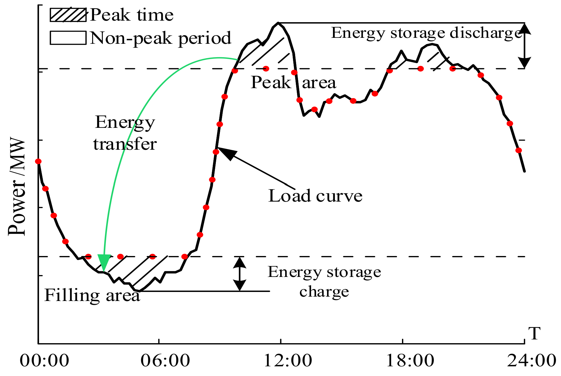
According to the peak regulation market, ES, as a third-party independent subject, needs to provide the output in strict accordance with the day-ahead power generation plan. Figure 1 is the schematic diagram of ES peak regulation. However, when the ES is only applied to a single peak load shaving scenario, it can only charge and discharge in the peak load period or the low load period, and remains idle in other periods, greatly reducing the ES utilization rate. Therefore, this paper adopts the method of “off-time reuse” for ES. In the non-peak regulating stage of ES, idle ES is used to improve the power grid frequency, and then improve the utilization rate. 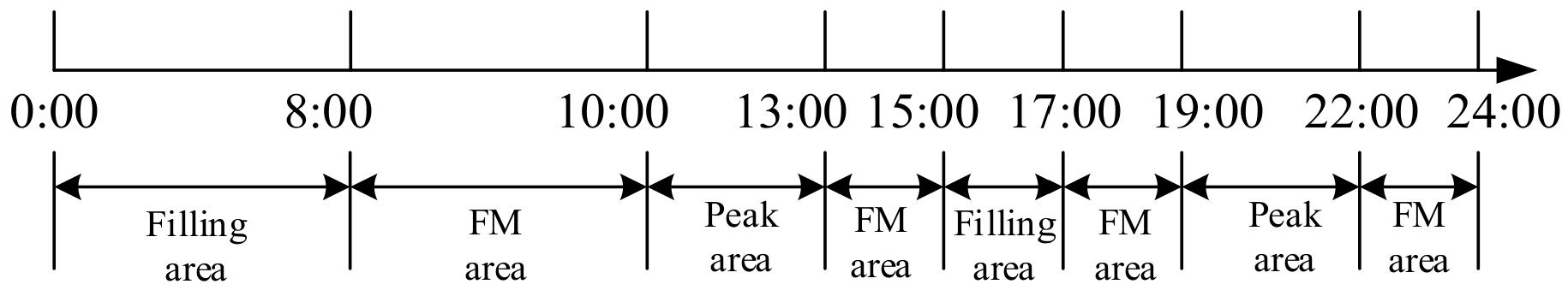According to the peak adjustment curve in Figure 1, ES can be divided into multiple working areas, as shown in Figure 2.

Figure 1 shows that the peak modulation frequency modulation state of the energy storage at a certain moment is unique, that is, the energy storage locks the energy storage frequency modulation function in the valley filling area or peak clipping area, while other idle time areas outside the peak modulation can participate in the frequency modulation scene. As shown in Figure 2, the working area of the collaborative scenario in which energy storage participates in peak-FM is valley filling area—FM area—peak clipping area—FM area connected end to end, fully improving the utilization rate of ES.

3. Multiscene Division and Coordination Control Strategy Based on SOC

Because ES operation is limited by installed capacity and SOC state. Therefore, this paper proposes an ES peak FM multiscene partitioning method and coordination control strategy based on SOC state.

(1)

SOC-based multi-scene division model of ES peak and FM

Based on the limited ES capacity, when ES is applied to peak-FM collaborative scenarios, it is necessary to reasonably plan the ES SOC to achieve the maximum utilization of ES. When the ES operates in the valley filling area, it enters the charging state, and the SOC can rise to 0.9. Meanwhile, when it operates in the peak clipping area, the SOC can be reduced to 0.1 when entering discharge state. 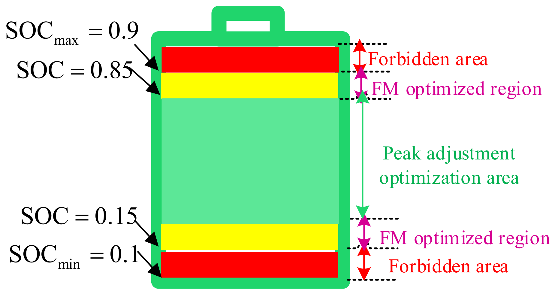Based on Figure 2, ES works end-to-end in multiple peak FM scenarios, including valley filling, frequency FM, peak clipping, and frequency FM. Therefore, when the ES switches from peak to FM state, the initial SOC value may be 0.1 or 0.9. However, the frequency deviation is bidirectional. Consequently, when SOC is 0.1, the ES cannot further discharge to improve the low frequency, and when SOC is 0.9, the ES cannot charge to improve the high frequency, which poses the hidden risk of low reliability. At the same time, considering the small capacity required by ES to participate in FM, the SOC in peak modulation scenario is set to 0.15–0.85 in this paper, and the SOC in FM scenario is set to 0.85 to 0.9 or 0.1 to 0.15, as shown in Figure 3.

(2)

Multiscene coordination control strategy

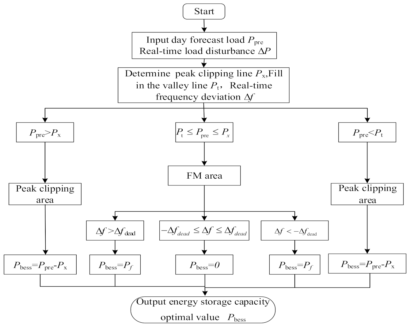
According to the above analysis, the realization process of a comprehensive control strategy for the collaborative scene of ES peak and FM is detailed as follows:

Step 1: import forecast load and real-time load disturbance data;

Step 2: determine the peak clipping line and the valley filling line based on predicted load data, and determine the frequency deviation based on real-time load disturbance data;

Step 3: when the predicted load data is outside the peak clipping line and valley filling line, it indicates that the ES is in the peak regulation area, and the ES output is determined according to the peak regulation control strategy;

Step 4: if the ES is not in the peak regulation zone, it is in the inner frequency regulation zone. Judge whether the frequency deviation crosses the dead zone; if it crosses it, determine the ES output according to the FM control strategy; otherwise, the ES output is 0;

Step 5: Output the optimal output value of ES. The multiscene coordination control strategy flow is shown in Figure 4.

4. ES Multiscenario Economic Scheduling Model

Based on the division method of energy storage scenarios in Section 3, it can be seen that energy storage only participates in a single scene in a certain period of time. Therefore, the multiscenario economic model of energy storage is the sum of single peak modulation scenario and single frequency modulation economic model. The objective function of the multiscenario economic optimization model of peak modulation and FM can be expressed as:

$$I=I_{\mathrm{total}-f}+I_{\mathrm{total}-p}$$

(1)

where I_total-f and I_total-p are the annual net benefits of monotone peak and single FM scenarios respectively. Among them, the single-scene economic model is as follows.

4.1. Single-Scenario Economic Optimization Model of ES Peak Shaving

The economic optimization model for the scenario of ES participating in peak shaving is mainly constructed from two aspects: investment cost and operating income. The investment cost mainly includes initial investment cost, operation and maintenance cost, and scrap cost.

(1)

Initial investment cost

Initial investment cost refers to the capital invested in the construction of an ES power station, which can be further divided into capacity cost and power cost. The formula is as follows:

$$C_t=\frac{M_p·P_m+M_E·E_m}{n}$$

(2)

where M_p denotes investment cost per unit power during the construction of ES power station, €/MW; M_E denotes investment cost per unit capacity, €/MWh; P_m denotes the rated power of the ES station, MW; E_m denotes the rated capacity of ES power station, MWh; n denotes the operating life of lithium iron phosphate battery ES power station, years.

(2)

Operation and maintenance costs

Operation and maintenance costs refer to the expenses dynamically invested in equipment overhaul and maintenance to ensure the normal operation of the ES power station, and is expressed as

$$C_y=N_p·P_m+N_E·E_m$$

(3)

where N_p denotes the maintenance cost per unit power of the ES station within its service life, €/MW; N_E denotes maintenance cost per unit capacity, €/MWh.

(3)

Scrap cost

This is the cost of cleaning up, destroying, and partially recovering the ES power station at the end of its service life, which has the following formula:

$$C_b=\frac{{\lambda }_{\mathrm{pcs}}·P_m-{\alpha }_{ecs}·E_m}{n}$$

(4)

where λ_pcs denotes the scrap cost of ES PCS per unit power, €/MW; α_ecs is the recovery cost of ES battery per unit capacity, €/MWh.

The operating benefits of ES involved in peak shaving include direct benefits and indirect benefits, as listed below. The direct income mainly involves peak load adjustment subsidy and peak load filling, and the indirect benefits mainly refer to environmental benefits, as well as delayed grid investment and construction benefits.

(1)

Revenue from peak cutting and valley filling:

$$I_{\mathrm{xf}}=\eta ·(P_{\mathrm{bess}-i}^{+}-P_{\mathrm{bess}-i}^{-})·\Delta t·P_{price}$$

(5)

where P_price is the difference in the real-time peak/valley electricity prices of the grid, η is the charging and discharging efficiency of ES, $P_{\mathrm{bess}-i}^{+}$ and $P_{\mathrm{bess}-i}^{-}$ respectively mean the discharge and charging power of ES at time i, and △t is the calculated time step.

(2)

Peak adjustment subsidy

The compensation standard of auxiliary services was clarified with the introduction of “two detailed rules” in China:

$$I_{tf}={\displaystyle \sum _{j=1}^{365}{\displaystyle \sum _{i=0}^n(P_{\mathrm{bess}-i}^{+}-P_{\mathrm{bess}-i}^{-})}·\Delta t·\varphi }$$

(6)

where $\varphi$ is the peak regulation subsidy standard, €/MWh.

(3)

Environmental benefits

Energy storage can assist with and reduce the peak load regulation power of the thermal power unit, thus reducing fuel and sewage costs.

$$E_{bess}={\displaystyle \sum _{i=0}^n{P}_{\mathrm{bess}-i}^{+}}·\Delta t$$

(7)

The environmental benefits of ES participating in peak shaving are calculated as shown in Equation (8):

$$I_{env}={\displaystyle \sum _{k=1}^{365}(E_{bess}·({\displaystyle \sum _{j=1}^m{G}_j}·R_j}))$$

(8)

where G_j denotes the emission of the j th pollutant, kg/MWh; R_j denotes the environmental control cost of the j th pollutant, €/kg; m is the number of pollutant types.

(4)

Delaying the income from power grid investment and construction

As the load increases, new equipment is needed to upgrade the distribution network. The load rate of the substation and the capacity demand of the distribution network can be reduced by building an ES station on the grid side and releasing electric energy at the peak load, replacing the traditional grid expansion scheme.

$$I_{delay}=\frac{C_{inv}·P_g·{(1-\frac{1+i_t}{1+i_d})}^n}{n}$$

(9)

where P_g denotes the capacity of power grid expansion delayed due to ES investment and construction, namely, the rated power of ES; C_inv denotes the cost of unit capacity expansion, which is €/MW; i_t and i_d represent the inflation rate and discount rate, respectively.

Overall, the economic optimization model of grid side ES participating in peak shaving is shown in Equation (10).

$$I_{\mathrm{total}-f}=I_{\mathrm{x}f}+I_{tf}+I_{env}+I_{delay}-C_t-C_y-C_b$$

(10)

4.2. Economic Optimization Model of Single-Scenario FM

Cost in the economic optimization model of ES participating in the FM scenario is similar to that in peak modulation scenario and will not be described here. The operation income mainly includes FM subsidy and reserve power income.

(1)

FM subsidy

According to the existing market mechanism of primary FM auxiliary service, a third-party independent entity provides economic subsidies according to its own power and capacity scale, such as

$$I_{\mathrm{S}}={\displaystyle \sum _{j=1}^{365}{\displaystyle \sum _{i=1}^n(P_{\mathrm{bess}-i}^{+}}+P_{\mathrm{bess}-i}^{-})·\Delta t·P_{\mathrm{PFR}}}$$

(11)

where PPFR denotes the subsidy of ES FM unit capacity, €/MWh.

(2)

Reserve power gain

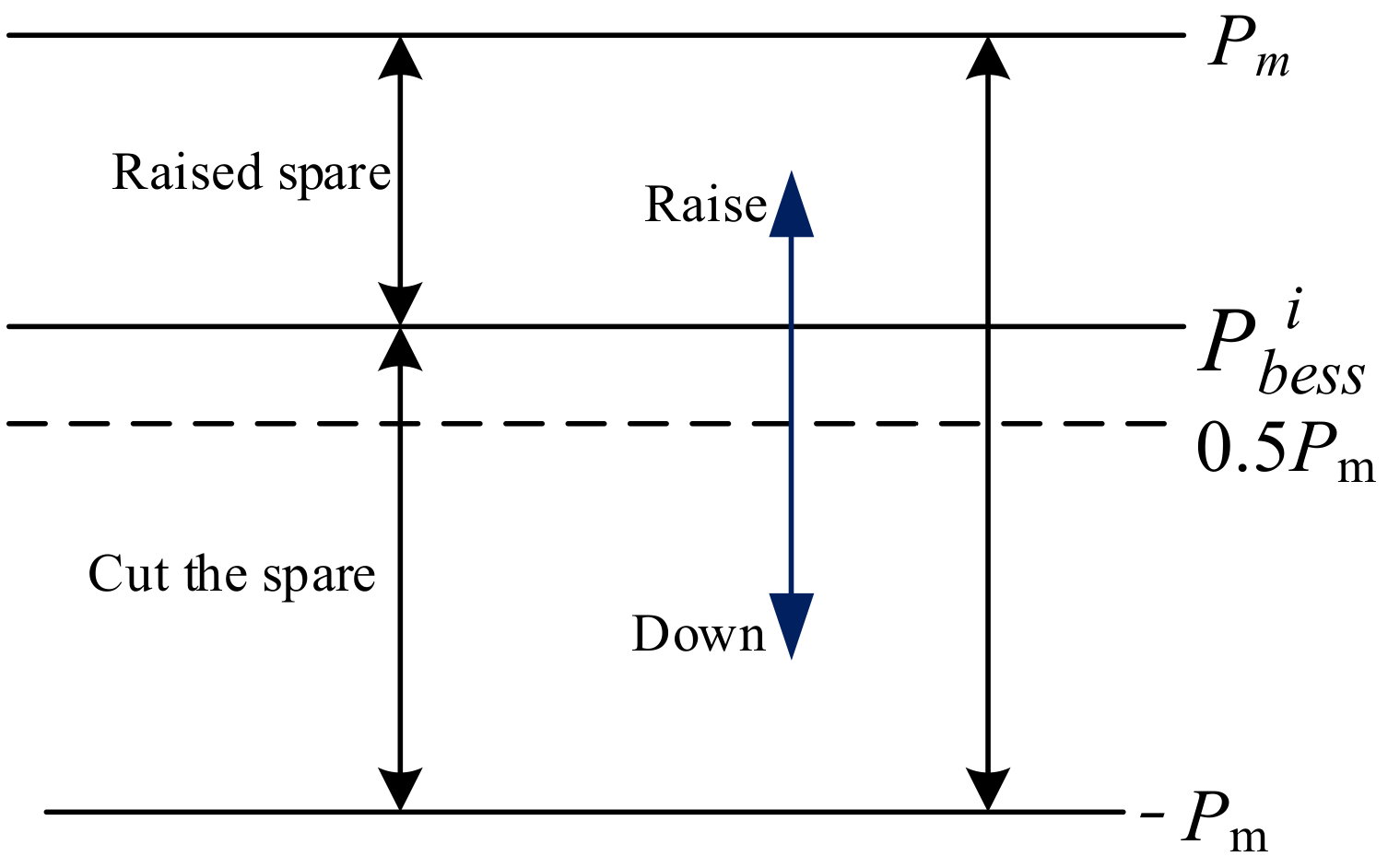
The reserve power of ES refers to the adjustable upper and lower power margin between the rated charge and the discharge power, which can be used as the reserve power of the grid to obtain benefits, as shown in Figure 5. The standby power is calculated according to Equations (12) and (13).

$$\left\{\begin{array}{l}{P}_{\mathrm{bess}-i}^{\mathrm{up}}=P_m-P_{\mathrm{bess}-i}^{+}\\ P_{\mathrm{bess}-i}^{\mathrm{dn}}=P_m+P_{\mathrm{bess}-i}^{-}\end{array}\right.$$

(12)

$$\left\{\begin{array}{l}{P}_{\mathrm{bess}-i}^{\mathrm{up}}=P_m+P_{\mathrm{bess}-i}^{-}\\ P_{\mathrm{bess}-i}^{\mathrm{dn}}=P_m-P_{\mathrm{bess}-i}^{-}\end{array}\right.$$

(13)

where $P_{\mathrm{bess}-i}^{\mathrm{up}}$ and $P_{\mathrm{bess}-i}^{\mathrm{dn}}$ are respectively the upregulated power and downregulated power of the ES system at moment i, MW.

Under normal circumstances, the ES can be both up- and downregulated, while it can only be charged when the ES SOC is too low, that is, it can only be downregulated. When the SOC is too high, it can only be discharged. The reserve power gain is settled in hours, and the time of up–down and down–down is evenly distributed, thus the reserve power gain is calculated as shown in Equation (14).

$$I_{res}={\displaystyle \sum _{j=1}^{365}\frac{1}{2}}·{\displaystyle \sum _{k=1}^{24}\left[C_{\mathrm{up}-k}({\displaystyle \sum _{i=60(k-1)+1}^{60k}\frac{P_{\mathrm{bess}-i}^{\mathrm{up}}}{60}})+C_{\mathrm{dn}-k}({\displaystyle \sum _{i=60(k-1)+1}^{60k}\frac{P_{\mathrm{bess}-i}^{\mathrm{dn}}}{60}})\right]}$$

(14)

where $C_{\mathrm{up}-k}$ and $C_{\mathrm{dn}-k}$ represent the price of ES standby power per hour, and the unit is €/MW.

In essence, the annual net income of ES on the grid side participating in the FM scenario is calculated as shown in Equation (15).

$$I_{total-p}=I_s+I_{res}-C_t-C_y-C_b$$

(15)

4.3. Model Constraints

(1)

Power constraint

Due to technical limitations of the battery body and PCS, the charging and discharging power of the ES cannot be greater than its set rated power. The power constraints are shown in Equations (16) and (17).

$$0\le P_{\mathrm{bess}-i}^{+}\le P_m$$

(16)

$$0\le P_{\mathrm{bess}-i}^{-}\le P_{\mathrm{m}}$$

(17)

(2)

Constraints on state of charge

The capacity of a given ES power station is limited. Overcharge and overdischarge will lead to the aging and failure of ES batteries. Therefore, the SOC of an ES power station needs to be constrained within a limited range. The calculation method of ES SOC is the ratio of the remaining capacity to the rated capacity. The ES SOC at time t is shown in Equation (18). To ensure the reliable operation of the ES power station, the SOC constraint is described in Equation (19).

$$\mathrm{SOC}(t)=\frac{E_0-{\displaystyle {\int }_0^i(P_{\mathrm{bess}-i}^{+}-P_{\mathrm{bess}-i}^{-})dt}}{E_m}$$

(18)

$${\mathrm{SOC}}_{\min }\le \mathrm{SOC}(t)\le {\mathrm{SOC}}_{\max }$$

(19)

where E₀ denotes the initial capacity of ES, MWh; E_m denotes the rated capacity of the ES station, MWh; SOC_min and SOC_max respectively denote the minimum and maximum values of ES SOC; the values of SOC_min and SOC_max are usually 0.1 and 0.9, respectively.

(3)

Balance constraint of ES charge and discharge amount

For the peak shaving scenario, it is necessary that the electric quantity released by peak shaving is equal to the electric quantity absorbed by valley filling within the daily time scale, that is, the ES needs to complete a full charge-discharge balance within a day, and the ES SOC needs to return to the initial state. The constraint of the charge-discharge balance is shown in Equation (20).

$${\displaystyle {\int }_0^n{P}_{\mathrm{bess}}^{+}}dt-{\displaystyle {\int }_0^n{P}_{\mathrm{bess}}^{-}}dt=0$$

(20)

4.4. Model Solution Based on Interior Point Method

The interior point method is a kind of penalty function method, which is suitable for nonlinear optimization problems, See [22] for the solving process.

$$\left\{\begin{array}{l}\begin{array}{cc}\min \hfill & f(x),x\in R\hfill \end{array}\\ \begin{array}{cc}s.t.& g_i\end{array}(x)\ge 0,i=1,\dots ,m.\end{array}\right.$$

(21)

The objective of this optimization model is to maximize the net benefit, and its feasible domain is shown in Equation (22).

$$D=\{x\in R|g_i(x)\ge 0,i=1,\dots ,m\}$$

(22)

The basic idea of this method is that each iteration point x is in the feasible region D, and when the iteration point is close to the boundary of the feasible region, the value of the augmented objective function increases suddenly to prevent the iteration point from crossing the boundary. Since the iteration point cannot reach the boundary but can only approach it infinitely, the feasible region is redefined as shown in Equation (23).

$$D_0=\{x\in R|g_i(x)>0,i=1,\dots ,m\}$$

(23)

The construction of the augmented objective function is shown in Equation (24).

$$H(x,\tau )=f(x)+\tau \overline{H}(x)$$

(24)

where $\overline{H}(x)$ is the barrier function, which needs to satisfy the case when the iteration point x approaches the boundary and the augmented objective function tends to infinity, thus it can be achieved that at least one of $g_i(x)$ needs to approach 0, and the logarithm of the constraint function is the barrier function, as shown in Equation (25).

$$\overline{H}(x)=-{\displaystyle \sum _{i=1}^m\ln [g_i(x)]}$$

(25)

The parameter $\tau$ is a penalty factor, which can constrain the value of $\overline{H}(x)$. When the iteration point x is in the feasible region D₀, the value of the obstacle function is limited. As x approaches the boundary, the barrier function approaches positive infinity, and there is a penalty.

The minimum value of optimization problems with constraints is generally at the boundary of the feasible region, hence the penalty factor should approach 0. This can be converted to solving the unconstrained optimization subproblem, and its expression is shown in Equation (26).

$$\begin{array}{cc}\min & H(x,{\tau }_k)=f(x)-{\tau }_k\end{array}{\displaystyle \sum _{i=1}^m\ln [g_i(x)]}$$

(26)

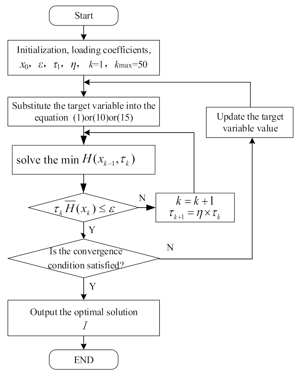
The process of solving the optimization model based on the interior point method is shown in Figure 6.

The specific solution steps are as follows:

Step 1: given the initial value, k = 1 and k_max = 50, iteration termination error $\epsilon$, initial penalty factor ${\tau }_1>0$, reduction coefficient $0<\eta <1$;

Step 2: solve the constructed unconstrained optimization subproblem and get the optimal solution of the objective function is obtained $I_k$;

Step 3: judge ${\tau }_k\overline{H}(x_k)\le \epsilon$ whether it is true. If it is true, it indicates that the extreme point meets the convergence condition, stop the calculation, and output $I_k$;

Step 4: if not, increase the number of iterations, $k=k+1$, reduce the penalty factor, ${\tau }_{k+1}=\eta \times {\tau }_k$, and go to Step 2 until the result meets the convergence condition.

5. Simulation Analysis

5.1. Simulation Parameters

To better illustrate the effectiveness of the proposed coordinated control method, the typical daily load data of a substation in a province in central China is taken as an example for simulation. The sampling interval of load disturbance data is 1 min, and there are a total of 1440 load disturbance data samples. The optimization variables to be solved include ES output, rated power Pm and rated capacity E_m at each moment (a total of 1442 moments). The frequency reference value is 50 Hz and the power reference value is 100 MW, P_x = 183.11 MW, P_t = 95.67 MW. The price is shown in

Table 2. Time-of-use electricity price (€/MWh).

Form	Critical Peak		Peak		Price Variance
	Period	Price	Period	Price
Great Industry	/	/	8:00–12:00 17:00–21:00	0.14	0.10
General Industry	/	/	8:00–12:00 17:00–21:00	0.18	0.13
Form	Usual		Off-peak
	Period	Price	Period	Price
Great Industry	12:00–7:00 21:00–4:00	0.08	0:00–8:00	0.04
General Industry	12:00–7:00 21:00–4:00	0.11	0:00–8:00	0.56

, the ES battery parameters are included in

Table 3. Parameters of lithium iron phosphate energy storage battery.

Charge and Discharge Depth	Cost of Power €/MWh	Capacity Cost €/MWh	Operational and Maintenance Cost €/MWh	Energy Density kWh/m3	Power Density kWh/m3
0.75	208.91	487.45	0.007	300	5500
Energy conversion efficiency	Power level kW	Response time	Duration of charge and discharge	Cycle life Number of times
92.5%	1~10,000	20 ms~2 s	1~2 h	2000

, and other parameters of the capacity optimization configuration model are set as indicated in

Table 4. Parameter values of capacity optimization model in peak and frequency modulation scenario.

Parameter	Numerical Value	Parameter	Numerical Value	Parameter	Numerical Value
Mp (€/MW)	208,907.83	n (Year)	10.5	PPFR (€/MW)	15.32
ME (€/MWh)	487,451.60	Cinv (€/MW)	417,815.66	KG	60
Np (€/MW)	2785.44	It (%)	1.5	KD	6
NE (€/MWh)	69.64	id (%)	4.5	λ	0.5
λpcs (€/MW)	974.90	α	0.5	γ	0.5
aecs (€/MWh)	3481.80	β	0.5

. In the analysis of environmental benefits, the types of environmental pollutants and corresponding unit treatment costs are shown in

Table 5. Types of emissions and environmental costs.

Gas Type	Parameter	Numerical Value	Parameter	Numerical Value
DUST	G1 (€/MWh)	0.07	R1 (€/kg)	0.41
SO2	G2 (€/MWh)	0.07	R2 (€/kg)	0.87
NOx	G3 (€/MWh)	0.10	R3 (€/kg)	1.12
CO2	G4 (€/MWh)	0.04	R4 (€/kg)	0.003
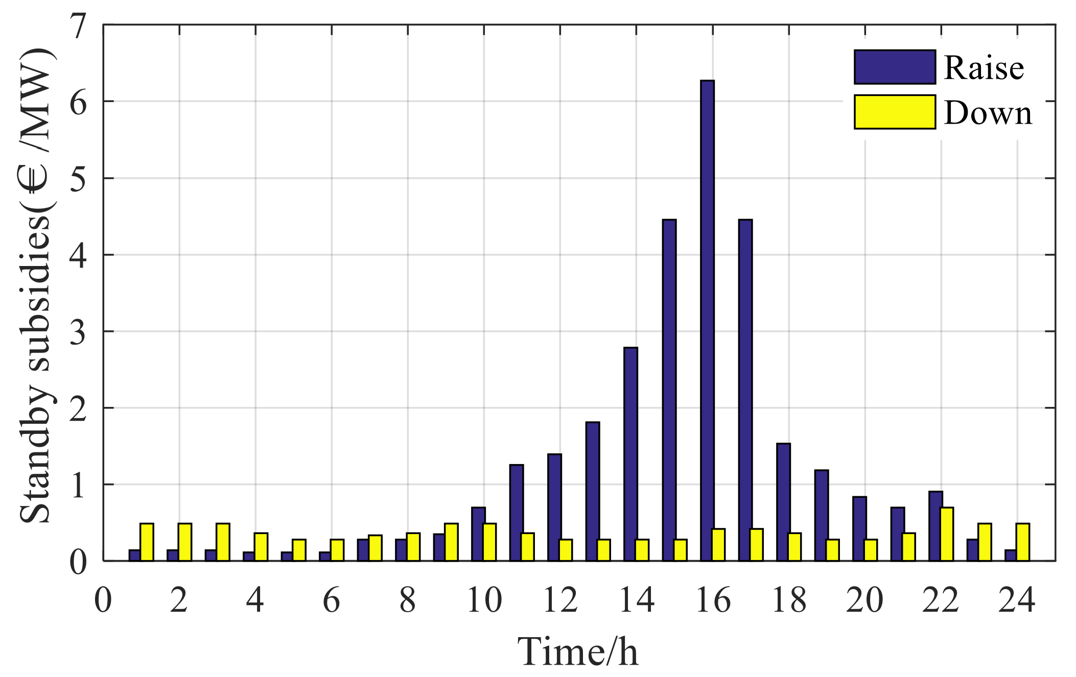
CO	G5 (€/MWh)	0.007	R5 (€/kg)	0.14

. The peak-shaving subsidy is referred to the implementation Rules for Grid-Connected Operation Management and Auxiliary Service Management of Electrochemical ES Power Stations in Southern China. The time-sharing subsidy price of FM standby capacity is shown in Figure 7.

5.2. Economic Analysis of Peak Shaving for Single Scenario

The maximum number of iterations is 500, and the iteration termination error ε is 10⁻¹⁰. The interior point method is used to solve the capacity configuration model of peak load balancing scenario aiming at economic optimization; the obtained optimal rated power P_m = 27.7 MW and rated capacity E_m = 80 MWh, and the annual net income of ES participating in peak load balancing scenario is €589,635.39. The corresponding annual cost and revenue is shown in

Table 6. Annual costs and benefits of energy storage participating in peak shaving scenario.

Annual cost of energy storage participating in peak shaving scenario	Initial investment cost	€4,265,619.34
	Operation and maintenance cost	€82,727.50
	Scrap cost	€−23,954.76
Annual revenue of energy storage participating in peak shaving scenario	Peak shaving subsidies	€4,586,641.04
	Environmental revenue	€48,884.43
	Delay grid investment construction income	€290,423.67
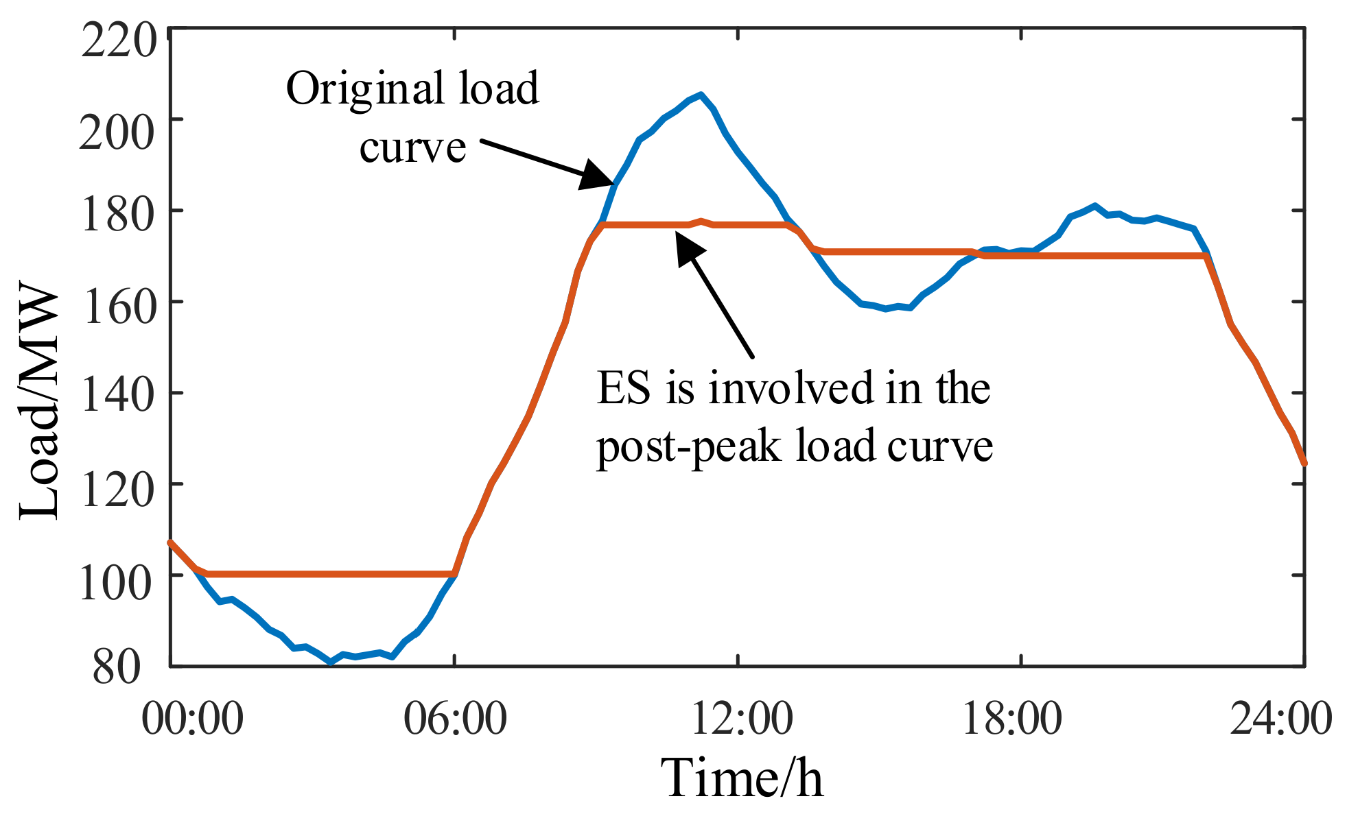
Annual net income of energy storage participating in peak regulation scenario		€602,169.86

, and the peak adjustment curve is presented in Figure 8.

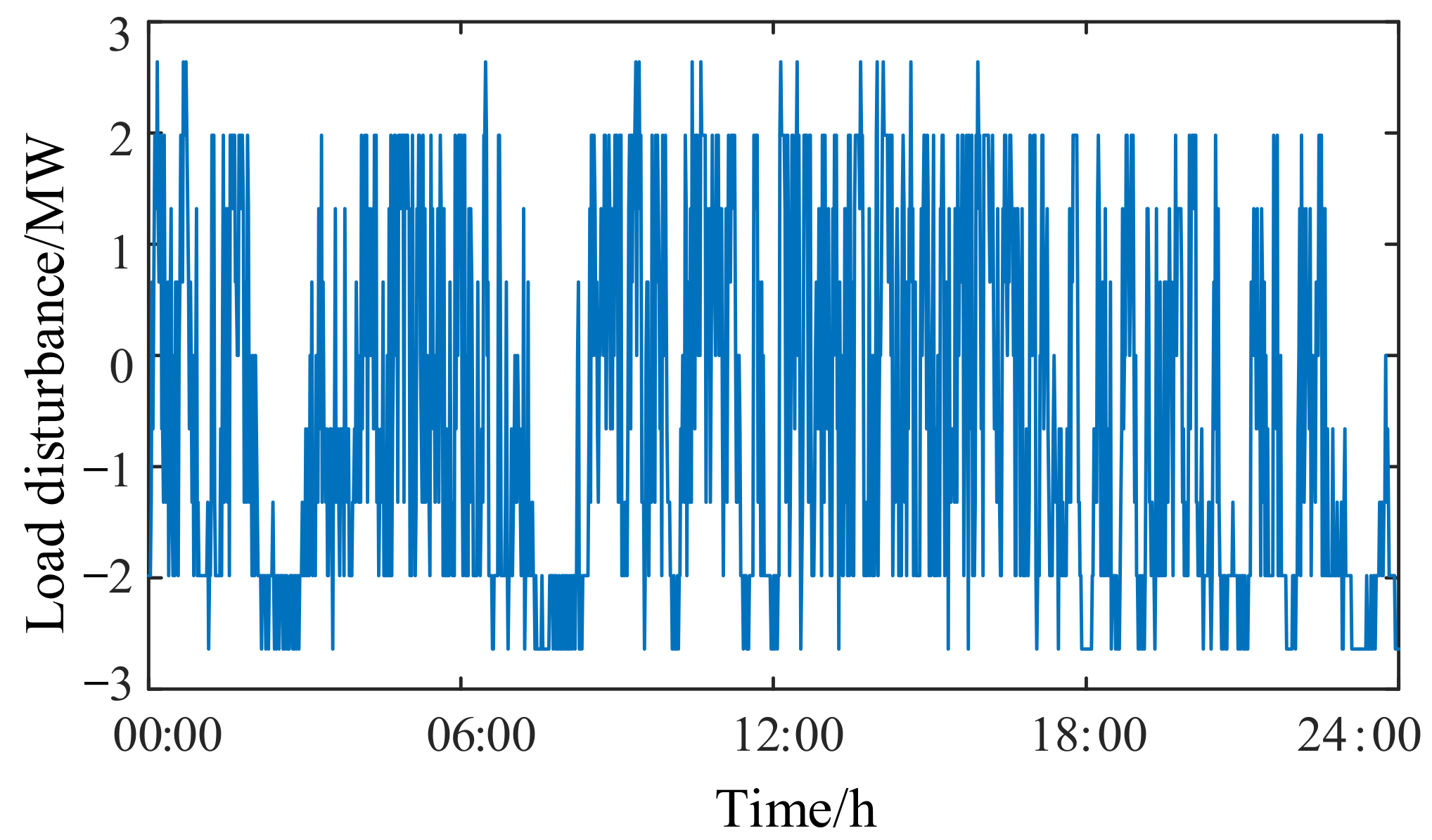
Figure 9 shows that the variance of the original load curve is 1499.4, and there are two obvious bulges, which are the afternoon peak from 10:00 to 13:00 and the evening peak from 19:00 to 22:00 respectively. Energy storage should release energy to relieve the power supply pressure of the power system. Industrial power consumption is the main power consumption in the afternoon peak, while residential power consumption is the main power consumption in the evening peak. Therefore, the load in the afternoon peak is higher than that in the evening peak. During 01:00~06:00 and 13:00~15:00, in the morning and lunch break respectively, the load curve is depressed, indicating that the power load is small and energy can be absorbed through energy storage.

After energy storage participated in peak regulation, the load variance was 978.5, 34.79% less than the original load variance data, indicating that energy storage participated in peak regulation and the curve was flatter after peak regulation. The peak value of the original load curve is 205.32 MW due to the effect of peak shaving and valley filling, the peak value of the load curve after ES is 177.24 MW, and the peak shaving rate reaches 13.68%, which alleviates the peak shaving pressure of the power grid. Combined with the data in Table 6, the initial investment cost accounts for a very high (about 98%) proportion of the total cost. The scrap cost includes the residual value generated by the recovery of ES battery resources, which is negative, indicating that the scrap cost can bring additional income. The peak adjustment subsidy accounts for 93.1% of the total income. The investment recovery period refers to the time required for the ES station to recover the costs. If ES only participates in peak adjustment, it will take 9.26 years.

5.3. Economic Analysis of Single-Scenario FM

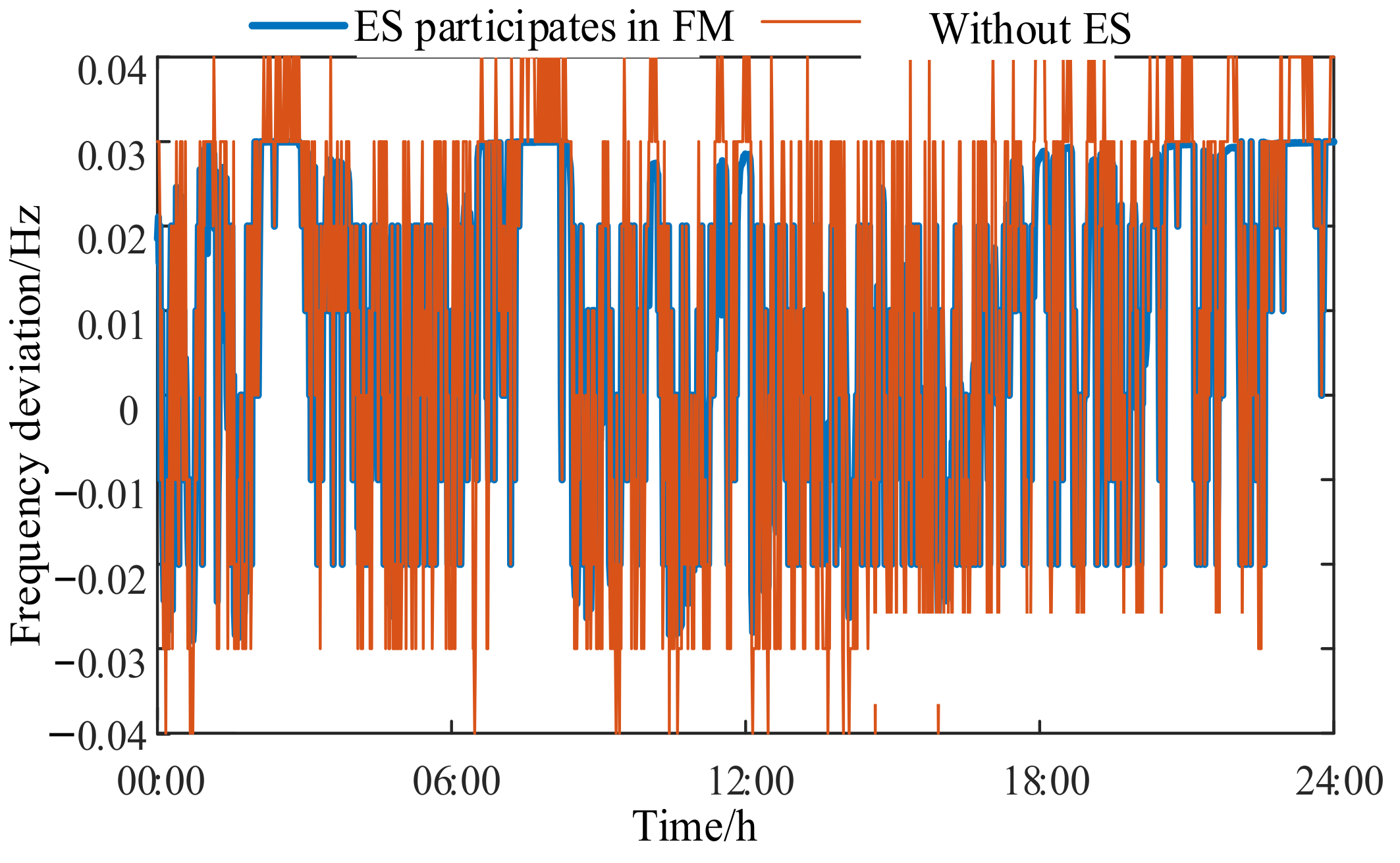
Under the working condition of load disturbance data shown in Figure 9, the com-parison between the original frequency deviation and the frequency deviation after energy storage frequency modulation is shown in Figure 10. The interior point method is used to solve the FM scenario based on the optimal objective of economy. The corresponding annual costs and annual benefits are listed in

Table 7. Annual costs and benefits of energy storage participation in power regulation scenarios.

Annual cost of energy storage participation in power regulation scenarios	Initial investment cost	€88,061.61
	Operation and maintenance cost	€5863.35
	Scrap cost	€−139.27
Energy storage participating in power regulation scenarios	Power regulation subsidies	€68,535.70
	Reserve power gain	€15,111
Energy storage participating in power regulation scenarios net annual revenue		€−10,819.06

.

Figure 10 shows that the load disturbance distribution has no obvious time characteristic and presents a random distribution state. Figure 3 and Figure 10 show that the proportion of the original load deviation crossing the dead zone is 54%, indicating that the period requiring frequency modulation accounts for about 54% of the whole day, and the demand for frequency modulation is large. The root mean square of frequency deviation of energy storage is 0.024 before energy storage participates in FM. After energy storage participates in FM, the system frequency deviation is significantly improved, and the root mean square value is 3.47 × 10⁻⁴, 88.5% lower than the original value, which also reflects the effectiveness of energy storage frequency modulation. The maximum absolute value of the original frequency deviation is 0.04 Hz, while the maximum absolute value of the frequency deviation after energy storage participates in the frequency modulation is 0.029 Hz, which is reduced by 27.5%, indicating that the frequency modulation effect is good.

According to Table 7, the initial investment cost accounts for about 93.7% of the total cost, and the residual value generated by ES battery resource recovery is greater than the scrap cost, which is negative. FM subsidy accounts for 81.9% of the total income, and the annual net income is negative, indicating that the investment cost cannot be recovered during the service life of the lithium iron phosphate battery storage power station. This indicates that ES is not profitable to participate in the FM scenario alone, which further verifies the necessity of ES to participate in the peak-FM collaborative scenario.

5.4. Economic Analysis of Multiple Scenarios of Peak Modulation and FM

According to the example analysis in Section 5.2 and Section 5.3, ES can effectively relieve the peak load regulation pressure of the power grid and improve its primary frequency regulation capacity. Therefore, the example in this section mainly verifies that the proposed coordinated control method can better improve ES utilization rate and reduce operating cost. The capacity configuration of the ES station is rated power P_m = 27.7 MW and rated capacity E_m = 80 MWh. 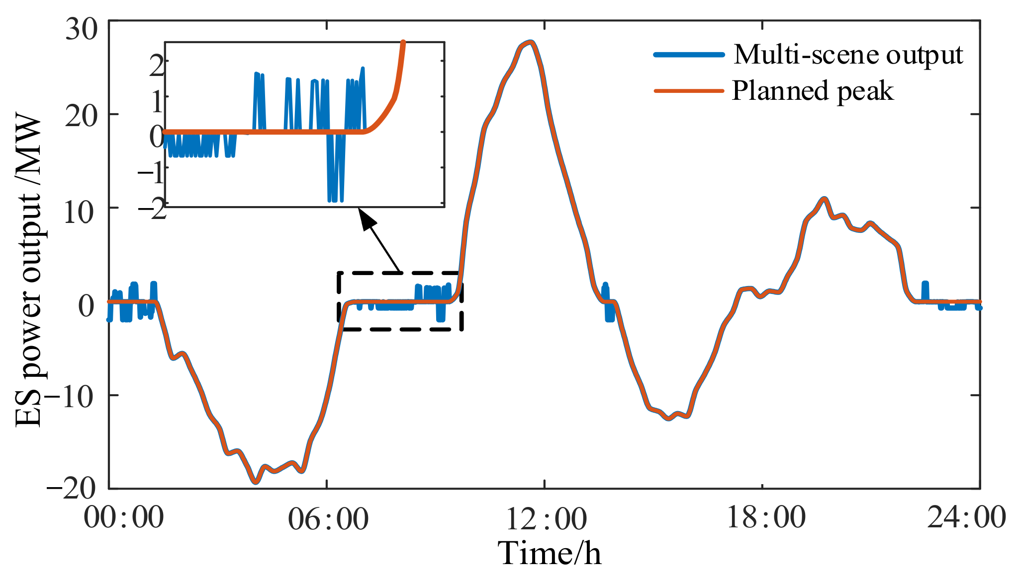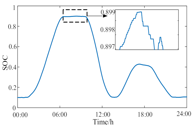Figure 11 shows the output value of ES in multiple scenarios involving peak modulation and FM, and Figure 12 depicts the SOC curve of ES.

Table 8. Energy storage utilization results for each scenario.

Scenario	Operation Time	Total Time	Usage Ratio
Peak shaving scenario	1082	1440	75.14%
Power regulation scenarios	779	1440	54.10%
Collaborative peak and frequency modulation scenarios	1316	1440	91.39%

includes the ES output data of single-scenario peak modulation, and single-scenario and multiscenario FM. The ES utilization rate in the table is the ratio of the accumulated output times to the total number of periods. The annual cost, annual revenue and annual net revenue in different scenarios are presented in

Table 9. Annual costs and benefits of energy storage in collaborative scenario of peak and frequency modulation.

Annual cost of energy storage participating in peak-frequency modulation collaborative scenario	Initial investment cost	€4,300,437.31
	Operation and maintenance cost	€82,727.50
	Scrap cost	€−24,219.38
Annual revenue of energy storage participating in peak-frequency modulation collaborative scenario	Peak shaving subsidies	€4,586,641.04
	Environmental revenue	€48,884.43
	Delay grid investment construction income	€290,423.67
	Power regulation subsidies	€21,043.98
	Reserve power gain	€42,199.38
Annual net income of energy storage participating in peak-frequency modulation collaborative scenario		€630,191.36

.

As can be seen from Figure 11, when ES participates in the coordinated control of multiple scenarios of peak modulation and FM, ES output power is consistent during peak modulation. In the FM period, when the system load increases, the ES discharges when the frequency decreases, and when the system load decreases, the ES charges when the frequency increases. Compared with that of single-scene, multiscene control can effectively improve ES utilization through the principle of “idle time reuse” of ES. The SOC of ES is always in the range of 0.1~0.9, and there is no SOC exceeding the limit, as shown in Figure 12, indicating that the configured capacity of ES meets the demand of the power grid.

Table 8 shows that the total number of ES outputs in a single peak shaving scenario is 1082, and the utilization rate is 75.14%. The total ES output times of single-scenario FM are 779, and the utilization rate is 54.10%. The peak and FM collaborative scenarios have the longest ES processing times, with a total of 1316, and ES utilization rate of 91.39%. Therefore, compared with single peak modulation and single FM scenarios, the utilization rate of coordinated control in multiple scenarios is increased by 16.25% and 37.29%, respectively. In terms of cost, there is a slight increase due to the rise of capacity demand, while in terms of revenue, ES participates in the FM scenario during the idle period, which can yield additional FM subsidy and standby power income, and the increased revenue partly exceeds the cost. Therefore, the annual net income increases by €28,021.50 compared with the single peak adjustment scenario, and the investment recovery life is shortened by 0.27 years to 8.99 years, as shown in Table 9.

6. Conclusions

ES only contributes to a single-scene (peak or FM) control of the power grid, resulting in low utilization rate and high economic cost. Herein, a coordinated control method of peak modulation and FM based on the state of ES under different time scales is proposed. The following conclusions can be obtained through simulation:

Based on the collaborative planning concept of a multipurpose, multimain, and multiauxiliary ES station, this paper proposes the coordinated control strategy of peak modulation and FM. Then, achieve the peak and frequency modulation working state switch. At the same time, the SOC in peak modulation scenario is set to 0.15–0.85 in this paper, and the SOC in FM scenario is set from 0.85 to 0.9 or 0.1 to 0.15; then, improve the reliability of peak frequency modulation.

Through the principle of “idle time reuse” of ES. Compared with that of mono-peak control and single-FM control, the ES efficiency of this method is increased by 16.25% and 37.29%, respectively. The annual net income is increased by €28,021.50, the investment recovery period is shortened by 0.27 years, and the ES configuration economy is effectively improved.

To sum up, the coordinated control of multiple peak-FM scenarios can not only raise the annual net income and reduce the investment recovery period, but also effectively improve the ES utilization rate. Furthermore, the double purpose of improving ES utilization rate and power grid economy can be realized.

References

- National Development and Reform Commission. The 13th Five-Year Plan for Renewable Energy Development. Available online: http://www.nea.gov.cn/2016-12/19/c_135916140.htm (accessed on 19 December 2016).
- National Development and Reform Commission, National Energy Administration. Strategy for Revolution in Energy Production and Consumption (2016–2030). Available online: https://www.ndrc.gov.cn/fggz/zcssfz/zcgh/201704/t20170425_1145761.Html (accessed on 29 December 2016).
- Olawumi, T.O.; Chan, D.W.M. A scientometric review of global research on sustainability and sustainable development. J. Clean. Prod. 2018, 183, 231–250. [Google Scholar] [CrossRef]
- Chen, C.; Li, X. Configuration Method and Multi-Functional Strategy for Embedding Energy Storage into Wind Turbine. Energies 2021, 14, 5354. [Google Scholar] [CrossRef]
- Li, Y.; Xu, Z.; Wong, K.P. Advanced control strategies of PMSG based wind turbines for system inertia support. IEEE Trans. Power Syst. 2017, 7, 3027–3037. [Google Scholar] [CrossRef]
- Varma, R.; Akbari, M. Simultaneous fast frequency control and power oscillation damping by utilizing PV solar system as PV-STATCOM. IEEE Trans. Sustain. Energy 2020, 1, 415–425. [Google Scholar] [CrossRef]
- Liu, Y.; Du, W.; Xiao, L. Sizing Energy Storage Based on a Life-Cycle Saving Dispatch Strategy to Support Frequency Stability of an Isolated System with Wind Farms. IEEE Access 2019, 7, 166329–166336. [Google Scholar] [CrossRef]
- Zhang, Y.J.; Zhao, C.; Tang, W.; Low, S.H. Profit-maximizing planning and control of battery energy storage systems for primary frequency control. IEEE Trans. Smart Grid 2018, 9, 712–723. [Google Scholar] [CrossRef] [Green Version]
- Barbour, E.; Wilson, I.A.; Radcliffe, J. A review of pumped hydro ES development in significant international electricity markets. Renew. Sustain. Energy Rev. 2016, 61, 421–432. [Google Scholar] [CrossRef] [Green Version]
- Dufo-López, R.; Bernal-Agustín, J. Techno-economic analysis of grid-connected battery storage. Energy Convers. Manag. 2015, 91, 394–404. [Google Scholar] [CrossRef]
- Hu, W.; Chen, Z.; Bak-Jensen, B. Optimal operation strategy of battery ES system to real-time electricity price in Denmark. In IEEE PES General Meeting; IEEE: Piscataway, NJ, USA, 2010; pp. 1–7. [Google Scholar]
- Murty, V.; Kumar, A. Multi-objective energy management in microgrids with hybrid energy sources and battery energy storage systems. Prot. Control. Mod. Power Syst. 2020, 5, 1–20. [Google Scholar] [CrossRef] [Green Version]
- Wu, Y.; Yang, W.; Hu, Y. Frequency Regulation at a Wind Farm Using Time-Varying Inertia and Droop Controls. IEEE Trans. Ind. Appl. 2019, 1, 213–224. [Google Scholar] [CrossRef]
- Wang, Z.; Wu, W. Coordinated Control Method for DFIG-Based Wind Farm to Provide Primary Frequency Regulation Service. IEEE Trans. Power Syst. 2018, 5, 2644–2659. [Google Scholar] [CrossRef]
- Liu, W.; Geng, G.; Jiang, Q. Model-Free Fast Frequency Control Support With Energy Storage System. IEEE Trans. Power Syst. 2020, 35, 3078–3086. [Google Scholar] [CrossRef]
- Mu, C.; Zhang, Y.; Jia, H. Energy-Storage-Based Intelligent Frequency Control of Microgrid With Stochastic Model Uncertainties. IEEE Trans Smart Grid 2020, 11, 1748–1758. [Google Scholar] [CrossRef]
- Shi, Y.; Xu, B.; Wang, D. Using battery storage for peak shaving and frequency regulation: Joint optimization for superlinear gains. IEEE Trans. Power Syst. 2017, 33, 2882–2894. [Google Scholar] [CrossRef] [Green Version]
- Dang, J.; Seuss, J.; Suneja, L. SOC feedback control for wind and ESS hybrid power system frequency regulation. IEEE J. Emerg. Sel. Top. Power Electron. 2014, 2, 79–86. [Google Scholar] [CrossRef]
- Xu, Q.; Xiao, J.; Peng, W. A decentralized control strategy for autonomous transient power sharing and state-of-charge recovery in hybrid ES systems. IEEE Trans. Sustain. Energy 2017, 8, 1443–1452. [Google Scholar] [CrossRef]
- Xu, Q.; Xiao, J.; Hu, X. A decentralized power management strategy for hybrid ES system with autonomous bus voltage restoration and state-of-charge recovery. IEEE Trans. Ind. Electron. 2017, 64, 7098–7108. [Google Scholar] [CrossRef]
- Mercier, P.; Cherkaoui, R.; Oudalov, A. Optimizing a battery ES system for frequency control application in an isolated power system. IEEE Trans. Power Syst. 2009, 24, 1469–1477. [Google Scholar] [CrossRef]
- Irisarri, G.; Kimball, L.M.; Clements, K.A. Economic dispatch with network and ramping constraints via interior point methods. IEEE Trans. Power Syst. 1998, 13, 236–242. [Google Scholar] [CrossRef]
Figure 1.
Schematic diagram of ES peak regulation.
Figure 2.
Division of collaborative working areas at different time scales.
Figure 3.
State definition of SOC.
Figure 4.
Control policy coordination flow in multiple scenarios.
Figure 5.
Schematic diagram of power up- and downregulation.
Figure 6.
Process of solving optimization model by interior point method.
Figure 7.
Compensation price of ES reserve.
Figure 9.
Load disturbance curve.
Figure 10.
Frequency deviation contrast.
Figure 11.
ES output in multiple peak and FM scenarios.
Figure 12.
ES SOC in multiple scenarios of peak and FM.