Battery State-of-Health Estimation Using Machine Learning and Preprocessing with Relative State-of-Charge

Abstract

Because lithium-ion batteries are widely used for various purposes, it is important to estimate their state of health (SOH) to ensure their efficiency and safety. Despite the usefulness of model-based methods for SOH estimation, the difficulties of battery modeling have resulted in a greater emphasis on machine learning for SOH estimation. Furthermore, data preprocessing has received much attention because it is an important step in determining the efficiency of machine learning methods. In this paper, we propose a new preprocessing method for improving the efficiency of machine learning for SOH estimation. The proposed method consists of the relative state of charge (SOC) and data processing, which transforms time-domain data into SOC-domain data. According to the correlation analysis, SOC-domain data are more correlated with the usable capacity than time-domain data. Furthermore, we compare the estimation results of SOC-based data and time-based data in feedforward neural networks (FNNs), convolutional neural networks (CNNs), and long short-term memory (LSTM). The results show that the SOC-based preprocessing outperforms conventional time-domain data-based techniques. Furthermore, the accuracy of the simplest FNN model with the proposed method is higher than that of the CNN model and the LSTM model with a conventional method when training data are small.

1. Introduction

The use of lithium-ion batteries has rapidly increased due to their low cost, high energy densities, low self-discharge rate, and long lifetime compared to other batteries [1,2,3,4]. Therefore, lithium-ion batteries have become prevalent in a variety of fields, such as mobile computing devices, aerospace devices, electric vehicles, and energy storage systems [5,6]. Even though lithium-ion batteries have notable advantages, a major downside is the capacity fade on repeated use. Furthermore, it is essential to monitor and estimate the capacity accurately, since an incorrect capacity estimation can cause permanent damage to the battery by overcharging or over-discharging [7]. The state of health (SOH) of a battery is a crucial indicator for evaluating the capacity fade of batteries. Therefore, it is essential to accurately estimate the SOH of lithium-ion batteries for guaranteeing the safety and reliability [8]. However, lithium-ion batteries are composed of complex chemical systems and are affected by the environment, for instance, the ambient temperature, resulting in complex calculations of their SOH [9]. Moreover, the nonlinear degradation of battery capacity challenges the SOH estimation and the remaining useful life (RUL) prediction [10].

Many studies have been conducted to determine an accurate estimation of the SOH. Generally, these studies can be classified into two categories: model-based methods and data-driven methods [11].

Model-based methods estimate the SOH of a battery by modeling the battery and considering the internal degradation process. Onori et al. [12] predicted the lifespan of a battery using a weighted ampere-hour throughput model of lithium-ion batteries and a severity factor map, which is used to determine the amount of damage that can occur to the battery. Plett [13] estimated the SOH of a battery using an equivalent circuit model and an extended Kalman filter, which automatically provides dynamic error bounds. Goebel et al. [14] predicted the lifespan of a battery through a linear relationship between the battery’s internal impedance and capacity using the particle filter approach. Wang et al. [15] proposed a method to predict the battery SOH using a state-space model depending on the discharge rate. Li et al. [16] estimated the SOH of a battery using an advanced single-particle model with electrolyte physics, considering internal mechanical and chemical battery degradation. Wang et al. [17] proposed a cell inconsistency evaluation model based on real-world operation data of electric vehicles. Although these model-based methods are useful for estimating the SOH of batteries, it is challenging to design an accurate aging model for lithium-ion batteries due to the highly complex chemical reactions inside the battery. Furthermore, the state of lithium-ion batteries is highly dependent on environmental factors, such as working temperature, anode materials, cathode materials, and others. Therefore, it is difficult to establish an exact aging model for lithium-ion batteries [18].

Data-driven methods have recently been drawing attention for SOH estimation due to their flexibility and effectiveness in non-direct observability. Data-driven methods predict the SOH of a battery using statistical or machine learning models. Hu et al. [19] introduced sparse Bayesian predictive modeling with a sample entropy of short voltage sequences to improve the accuracy of the estimation. Piao et al. [20] proposed a hidden Markov model to estimate and analyze the SOH of a battery. Liu et al. [21] used Gaussian process regression, which combines the covariance functions and mean functions to estimate the SOH. Liu et al. [22] also proposed an optimized relevance vector machine algorithm to estimate the RUL of a battery. Jin et al. [23] predicted the short-term SOH and long-term RUL of lithium-ion batteries with indirect health indicators and the Gaussian process regression model. Patil et al. [24] used a support vector machine as the battery SOH estimator with critical features from battery cycling data. Khumprom and Yodo [25] presented the data-driven prognostic using deep neural networks to predict the SoH and the RUL of the lithium-ion battery. Xia and Abu Qahouq [26] proposed an adaptive SOH estimation method utilizing a feedforward neural network (FNN) and online AC complex impedance. She et al. [27] proposed a prediction method for a battery aging assessment using a radial basis function (RBF) neural network with an incremental capacity analysis. Eddahech et al. [28] showed that recurrent neural networks can be used to predict performance decline in batteries. Tian et al. [29] proposed a deep neural network to estimate charging curves of batteries from which SOH can be computed. Shen et al. [30] proposed a method to predict the usable capacity of a battery using a deep convolutional neural network (CNN) with current and voltage measurement data. Park et al. [31] combined multichannel charging profiles and a long short-term memory (LSTM) model to improve the accuracy of an RUL prediction. The data-driven method can predict the SOH of a battery without electrochemical knowledge of the battery’s internal structure and aging mechanisms. Therefore, these methods can be easily implemented without information on the electrochemical characteristics of a battery and the environmental factors. Despite such remarkable success, most studies have only focused on steps taken to develop a statistical model or machine learning model—such as introducing a complex model and additional parameters—to improve the estimation accuracy. Therefore, the primary limitation is the inefficiency of training models and their inaccuracy in predicting the SOH because they do not consider the characteristics of the battery.

In this work, we develop an efficient preprocessing method to improve the accuracy and efficiency of SOH estimation in machine learning models, considering the fact that the battery characteristics are affected by the battery’s energy level. The proposed preprocessing method consists of a relative state of charge (SOC) and conversion, transforming the time-domain data into SOC-domain data. This simple preprocessing method increases the accuracy and efficiency of the estimation in the same machine learning model. Furthermore, when training data are small, the proposed method improves the SOH estimation accuracy of the simplest FNN model, which is higher than that of the complex models with a conventional method.

The remainder of this paper is organized as follows: In Section 2, we provide a brief description of battery datasets. In Section 3, we present a new preprocessing method for SOH estimation and comparison with conventional time-based data processing methods. In Section 4, we describe the machine learning process for SOH estimation using the proposed preprocessing method. In Section 5, we compare the SOH prediction results of preprocessing based on the constant time interval and preprocessing based on the SOC basis. The conclusions are presented in Section 6.

2. Battery Dataset

In this study, the lithium-ion battery dataset for SOH estimation was obtained from the NASA Prognostics Center [32]. As shown in Figure 1, we selected four batteries labeled #5, #6, #7, and #18 that were widely used for SOH estimation [18,25,33]. This dataset consisted of operating profiles and measured the impedance of 18,650 lithium-ion batteries when charging and discharging at room temperature. The batteries were charged at a constant 1.5 A until the charging voltage reached 4.2 V and, then, continued to charge at a constant 4.2 V until the charging current dropped below 20 mA. The batteries were discharged at a constant current of 2 A until the voltage of the battery dropped to 2.7 V, 2.5 V, 2.2 V, and 2.5 V for batteries #5, #6, #7, and #18, respectively.

Because each battery had a different initial capacity, as shown in Figure 1, the health of batteries was evaluated using the SOH. There are several methods for calculating the SOH; however, there are mainly two methods based on the battery’s impedance and the battery’s usable capacity [34,35]. The method defined by the impedance of the battery is not suitable for an online measurement because it requires instruments such as electrochemical impedance spectroscopy. Therefore, in this study, we used the SOH of a battery based on its usable capacity. This method can be expressed as follows [36]:

$$SOH=\frac{C_{usable}}{C_{rated}}$$

(1)

where $C_{usable}$ is the usable capacity which represents the maximal releasable capacity when it completely discharged, while $C_{rated}$ is the rated capacity, which is provided by the manufacturer. The usable capacity declines over time.

3. Proposed Preprocessing Method

We proposed a new preprocessing method that consisted of a relative SOC and data processing that transforms time-domain data into SOC-domain data. The time-domain data of batteries are among the most widely used data for SOH estimation because they are typically measured at constant intervals. However, battery characteristics are dependent not on time intervals, but on their internal energy, which is related to the SOC.

3.1. Relative State of Charge

The typical SOC of a battery is related to its stored energy and was calculated based on the design capacity [37] as follows:

$$SO{C}_{typical}\left(t\right)=\frac{C\left(t\right)}{C_{rated}}$$

(2)

where $C_{rated}$ is the design capacity and $C\left(t\right)$ is the current capacity at time t. However, complex calculations or measurements were required to estimate the typical SOC accurately. The purpose of our study was to improve machine learning models of SOH estimation using the data preprocessing that can be simply computed based on the relationship between battery characteristics and its energy level. It was not essential to use a typical SOC, and we needed indicators related to the energy level of the battery. Consequently, we introduced a relative SOC—simply called SOC—which was correlated with the battery’s energy level. The relative SOC was calculated simply by the usable capacity during the charging process as follows:

$$SO{C}^k\left(t\right)=SO{C}^k\left(t_0\right)+\frac{1}{C_{usable}^k}{\int }_{t_0}^t{I}_{c}dt$$

(3)

where $t_0$ is start time, t is current time, $C_{usable}^k$ is the usable capacity computed, and $I_c$ is the charging current at the k-th cycle. The usable capacity could be computed by integrating the current as follows [38]:

$$C_{usable}^k={\int }_{t_0}^{t_{cutoff}}{I}_{d}dt$$

(4)

where $t_0$ is the discharging start time, $t_{cutoff}$ is the time when the battery voltage is below the cutoff voltage, $I_d$ is the discharging current from the battery at k-th cycle, and $C_{usable}^0$ is set to $C_{rated}$. The relative SOC was easily computed during the battery charging and had a value between 0% and 100%, even if the battery was degraded. Therefore, in this paper, we discussed how to process data based on the relative SOC.

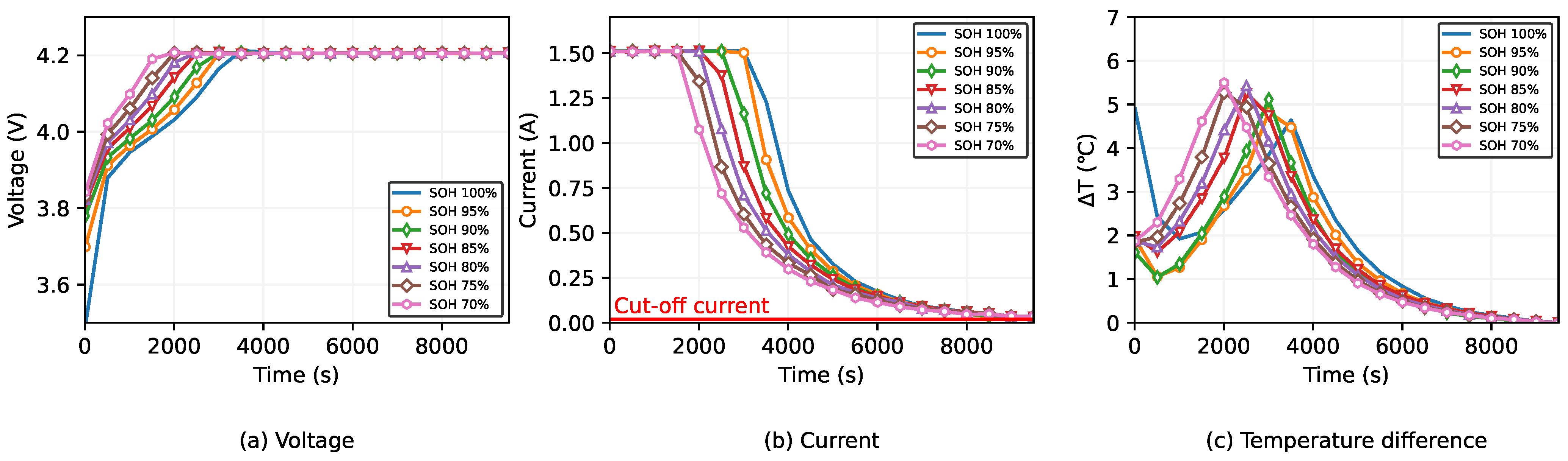
3.2. Time-Based Data Sampling

Many studies have used the time-based data sampling, in which data are collected by constant time interval [31,33,39]. Their approach seemed reasonable, as typical equipment is measuring data at constant time interval. For comparison with the proposed SOC-based method, we generated data using the same elements based on time-based data sampling. The dataset sampled by a constant time interval consisted of time, voltage, current, temperature difference, and cycles, as follows:

$$D_{timebase\#n}^k=\left(\begin{array}{cccc}{t}_1^k& t_2^k& \dots & t_s^k\\ V_1^k& V_2^k& \dots & V_s^k\\ I_1^k& I_2^k& \dots & I_s^k\\ \Delta T_1^k& \Delta T_2^k& \dots & \Delta T_s^k\\ k& k+\frac{1}{s-1}& \dots & k+1\end{array}\right)$$

(5)

where $t_m^k,V_m^k,I_m^k,$ and $\Delta T_m^k$ are the m-th sampling points of time, voltage, current, and temperature difference at the k-th cycle in the n-th battery dataset, and s is the total number of sampling points during one charge cycle. The temperature difference was calculated as follows:

$$\Delta T_m^k=T_m^k-min\left({\mathbf{T}}^{\mathbf{k}}\right)$$

(6)

where k is number of cycles, m is m-th sampling points, and ${\mathbf{T}}^{\mathbf{k}}$ is a collection of temperature measured at k-th cycle.

Figure 2 shows the sampling data of voltage, current, and temperature difference by constant time interval during charging of battery #5 with a total of 20 sampling points during one charge cycle. Figure 2a shows that the voltage of the aged battery reached 4.2 V faster than newer ones. However, regardless of their health condition, the battery’s voltage maintained the same 4.2 V after 4000 s. Therefore, almost 65% of voltage data had the same values. Similarly, a significant difference was not found in the current value in less than 4000 s or over 6000 s. The change in temperature difference of battery #5 was also slightly different after 6000 s. This result showed that the preprocessing based on time-domain features was insufficient to indicate the battery’s health state.

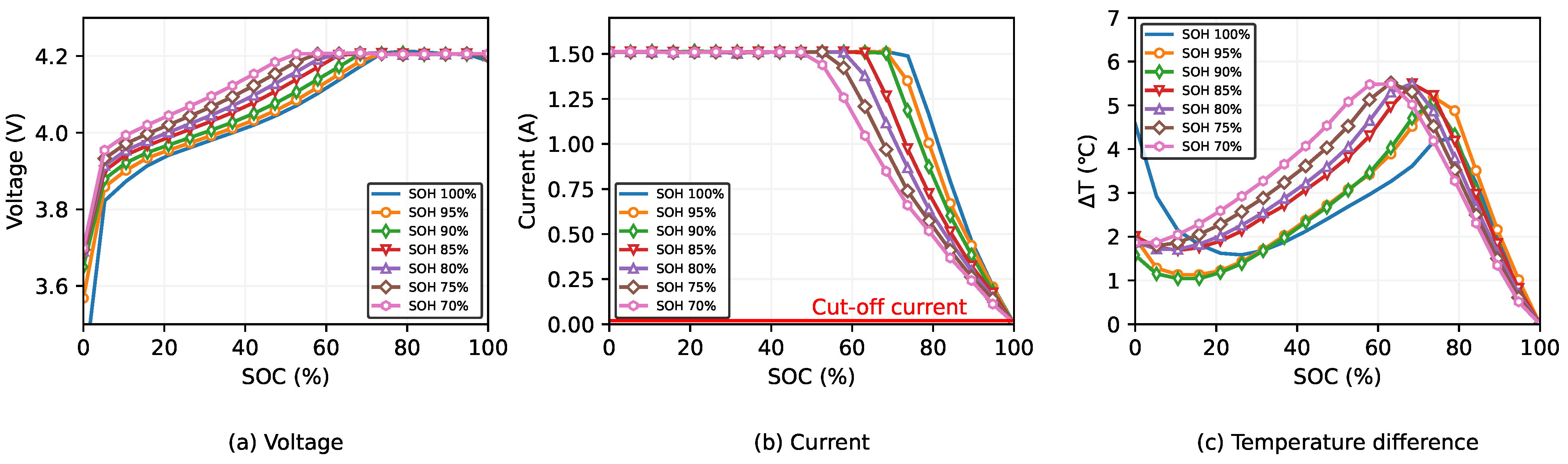
3.3. SOC-Based Data Sampling

The relative SOC is correlated with the battery’s energy, and the characteristics of the battery are affected by the battery’s energy level. For this reason, we introduced SOC-based data sampling. The SOC-based data sampling is the method by which data are collected by constant relative SOC interval, considering the battery’s energy. The dataset sampled by a constant relative SOC interval consisted of relative SOC, voltage, current, temperature difference, and cycles, as follows:

$$D_{socbase\#n}^k=\left(\begin{array}{cccc}SO{C}_1^k& SO{C}_2^k& \dots & SO{C}_s^k\\ V_1^k& V_2^k& \dots & V_s^k\\ I_1^k& I_2^k& \dots & I_s^k\\ \Delta T_1^k& \Delta T_2^k& \dots & \Delta T_s^k\\ k& k+\frac{1}{s-1}& \dots & k+1\end{array}\right)$$

(7)

where $SO{C}_m^k,V_m^k,I_m^k,$ and $\Delta T_m^k$ are the m-th sampling points of the relative SOC, voltage, current, and temperature difference at the k-th cycle in the n-th battery dataset, and s is the total number of sampling points during one charge cycle. The temperature difference was calculated as Equation (6).

Figure 3 shows data sampled by constant relative SOC interval of battery #5 with a total of 20 sampling points during one charge cycle. Compared to Figure 2, the data preprocessed based on SOC basis differed for the aged battery and the new battery. Notably, the battery’s voltage sampling values had a significant difference between 0% and 70%. This value was 40% higher than the time-based preprocessing, showing only a 30% difference in voltage data between the old and new batteries. Figure 3 also shows that current and temperature variation in preprocessing based on SOC values was highly correlated with the SOH of the battery.

3.4. Correlation Analysis

Figure 4 shows the heatmap of the Pearson correlation coefficient between the usable capacity and sampling data. In Figure 4, the data in SOC-based datasets correlated highly with capacity compared to time-based datasets. In particular, the voltage data in SOC-based datasets were more correlated with the usable capacity than the voltage data in time-based datasets. Furthermore, the correlation coefficient between the usable capacity and the temperature difference in SOC-based datasets was higher than in time-based datasets.

Table 1. Average absolute values of the Pearson correlation coefficient and the ratio of highly correlated variables according to the data processing method (sampling number = 20).

	Battery #5		Battery #6		Battery #7		Battery #18
Preprocessing Method	Timebase	SOCbase	Timebase	SOCbase	Timebase	SOCbase	Timebase	SOCbase
Average absolute value	0.39	0.54	0.44	0.55	0.38	0.46	0.33	0.40
Ratio of highly correlated variables *	35%	55%	37%	55%	33%	42%	23%	30%

* The magnitude of the correlation coefficient was between 0.7 and 1.0.

represents the average absolute values of the correlation coefficient and the ratio of highly correlated variables, whose magnitude was between 0.7 and 1.0, according to various battery datasets and data processing methods. Table 1 shows that the ratio of highly correlated variables in SOC-based datasets was higher than in time-based datasets. In addition, the average absolute values of the correlation coefficient in SOC-based datasets were higher than in time-based datasets. This result established that the SOC-based data processing was more correlated with the usable capacity than the time-based data processing.

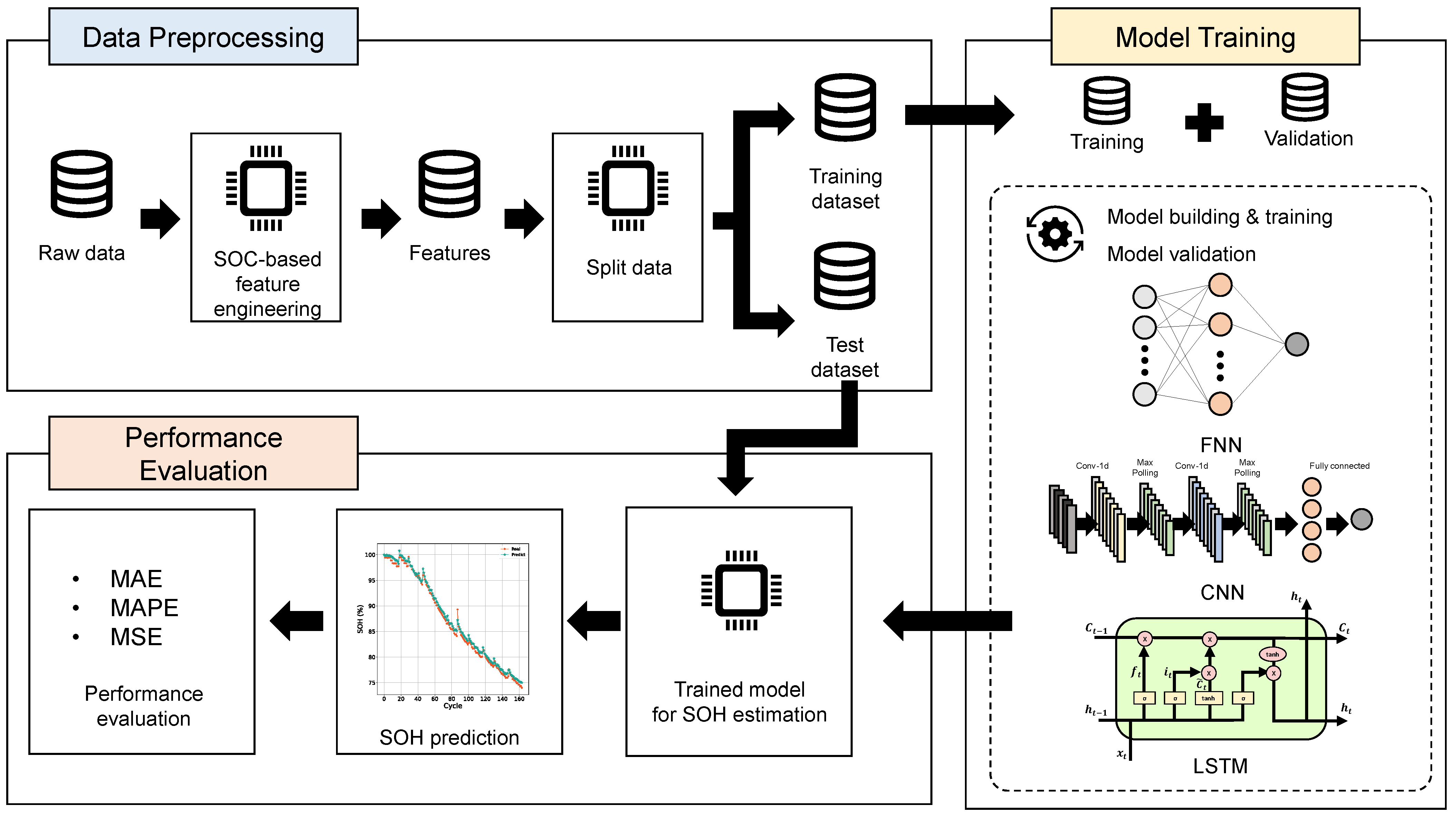
4. Machine Learning Process

As shown in Figure 5, the proposed process for battery’s SOH estimation consisted of three stages: data preprocessing, model training, and a performance evaluation. The missing and abnormal values were removed from the batteries’ raw data during the data preprocessing stage. After data cleaning, the time-based data were transformed into SOC-based data, and the features of the battery were extracted. The feature data were split into a training dataset and test dataset. In the model training stage, the training dataset was split into training data and validation data. We trained FNNs, CNNs, and LSTMs using the training data. The hyper-parameters of the architecture were adjusted using the validation data. In the performance evaluation stage, the trained model was tested using the test dataset, and its performance was evaluated using the mean absolute error (MAE), mean absolute percentage error (MAPE), and mean squared error (MSE).

4.1. Data Preprocessing

Data preprocessing was performed to obtain data suitable for a machine-learning model. Data cleaning was performed because the raw data contained abnormal and missing values. The raw data, based on time series, was transformed into SOC-based data after data cleaning, and features were extracted from SOC-based data. The feature format was expressed in Equation (7). The SOC-based dataset did not have the same scale. Therefore, we normalized the SOC-based dataset using min–max normalization [40] as follows:

$$z_{nm}^k=\frac{x_{nm}^k-min\left({\mathbf{x}}_{\mathbf{n}}\right)}{max\left({\mathbf{x}}_{\mathbf{n}}\right)-min\left({\mathbf{x}}_{\mathbf{n}}\right)}n\in \{1,\dots ,5\},m\in \{1,\dots ,s\}$$

(8)

where k is the number of cycles, m is m-th sampling point, and ${\mathbf{x}}_{\mathbf{n}}$ is a collection of the n-th row in Equation (7) of all charging cycles. Furthermore, we normalized the capacity using min–max normalization, as follows:

$$c^k=\frac{C^k-min\left(\mathbf{C}\right)}{max\left(\mathbf{C}\right)-min\left(\mathbf{C}\right)}$$

(9)

where k is the number of cycles and $\mathbf{C}$ is a collection of capacities for all charging cycles. After normalization, we split the data into the training dataset, to fit the model parameters, and the test dataset, to test the final models.

4.2. Model Training

In the model training stage, we split the training dataset into training data and validation data. We applied the SOC-based dataset to three different machine learning models: FNN, CNN, and LSTM architectures. The model structures are summarized in

Table 2. Structure and parameters of neural networks.

Model	Structure	Number of Sampling Points	Number of Parameters
FNN	Input → Hidden (Neurons: 40) → Output	20	4081
		40	8081
		100	20,081
		200	40,081
CNN	Input →	20	8441
	Conv1d (Channel:20/Kernel:3) →MaxPool1d (Kernel:2/Stride:2) →	40	16,441
	Conv1d (Channel:40/Kernel:4) →MaxPool1d (Kernel:2/Stride:2) →	100	40,441
	FC (Neurons: 40) → Output	200	80,441
LSTM	Sequence: 4 Number of recurrent layers: 1 Hidden Size: 60	20	38,941
		40	62,941
		100	134,941
		200	254,941

.

4.2.1. System Configuration

The training dataset was divided into training data and validation data, and the ratio of the training data to the validation data was two to one. The simulation was implemented using PyTorch 1.7, and calculated using GeForce GTX 1080Ti. The loss function for training was expressed as the MSE as follows:

$$MSE=\frac{1}{N}\sum _{i=1}^N{(C_i-{\widehat{C}}_i)}^2$$

(10)

where $C_i$ is the actual capacity, $\widehat{C_i}$ is the estimated capacity, and N is the number of datasets. We adopted the AdamW optimizer [41], and the initial learning rate was ${10}^{-3}$ for the FNN and ${10}^{-4}$ for the CNN and the LSTM.

4.2.2. Feedforward Neural Network (FNN)

The FNN is an artificial neural network, which is an acyclic graph, and is the simplest neural network. The FNN, which is essential for machine learning to form the basis of many architectures, consists of multiple layers of perceptrons with a nonlinear activation function [42]. We employed the simplest structure of the FNN, which had a three-layer structure, consisting of an input, hidden, and output layers. The input layer had neurons of the same size as the matrix in Equation (7). The hidden layer contained 40 hidden neurons, and the hyperbolic tangent function was used as an activation function. The dropout rate for regularization was set to 20%.

4.2.3. Convolutional Neural Network (CNN)

The CNN, which employs a mathematical convolution operation, is a specialized type of FNN for processing gird-like data. A layer of convolutional networks consisted of three stages. In the first stage, the convolution operation, in a 1-D discrete case, was performed in parallel [42] as follows:

$$s\left(t\right)=(x\ast w)\left(t\right)=\sum _{a}x\left(a\right)w(t-a)$$

(11)

where x is an input matrix, w is a kernel matrix, and ∗ is the convolution operator. In the second stage, each result of the convolution operation was run through a nonlinear activation function, namely, the hyperbolic tangent. In the third stage, a max-pooling function was performed on the results. Two layers of convolutional networks and fully connected layers with 40 hidden neurons were required, as shown in Table 2. The dropout rate for regularization was set to 20%.

4.2.4. Long Short-Term Memory (LSTM)

The LSTM is a special kind of recurrent neural network (RNN) that allows outputs at each time step to be used as inputs for processing sequential data. The difference between LSTM and simple RNN is that the weight on the self-loop is conditioned on the context rather than fixed [42]. Cells in LSTM are connected recurrently to each other. Input values calculated with a regular neuron unit can be accumulated in the state if the input gate allows it. The state unit has a self-loop controlled by the forget gate, and the output gate can block the output of the LSTM cell. The LSTM was calculated [43] as follows:

$$\begin{array}{c}{f}_t=\sigma (W_f{x}_t+U_f{h}_{t-1}+b_f)\end{array}$$

(12)

$$\begin{array}{c}{i}_t=\sigma (W_i{x}_t+U_i{h}_{t-1}+b_i)\end{array}$$

(13)

$$\begin{array}{c}{o}_t=\sigma (W_o{x}_t+U_o{h}_{t-1}+b_o)\end{array}$$

(14)

$$\begin{array}{c}{\tilde{c}}_t=tanh(W_c{x}_t+U_c{h}_{t-1}+b_c)\end{array}$$

(15)

$$\begin{array}{c}{c}_t=f_t\circ c_{t-1}+i_t\circ {\tilde{c}}_t\end{array}$$

(16)

$$\begin{array}{c}{h}_t=o_t\circ tanh\left(c_t\right)\end{array}$$

(17)

where $x_t$ is the input vector, $f_t$ is the activation vector of the forget gate, $i_t$ is the activation vector of the input and update gates, $h_t$ is the hidden state vector, ${\tilde{c}}_t$ is the activation vector of the input of the cell, $c_t$ is the cell state vector, $W/U$ is the weight matrix, and b is the bias; the initial values were $c_0=0$ and $h_0=0$, and the operator ∘ denoted the Hadamard product, which was an element-wise product.

4.3. Performance Evaluation

To evaluate the performance of the models, the MSE was calculated from the test data. In addition, the MAE and MAPE were computed for a performance evaluation as follows:

$$\begin{array}{c}MAE=\frac{1}{N}\sum _{i=1}^N|C_i-{\widehat{C}}_i|\end{array}$$

(18)

$$\begin{array}{c}MAPE=\frac{100\%}{N}\sum _{i=1}^N\left|\frac{C_i-{\widehat{C}}_i}{C_i}\right|\end{array}$$

(19)

where $C_i$ is the actual capacity, $\widehat{C_i}$ is the estimated capacity, and N is the number of datasets.

5. Experiment Results

5.1. Sampling Size

There were various methods to choose sampling points for charging. As the number of sampling points increased, more information was contained within the sample. However, the machine learning models would require more parameters, and not all sampling points were essential for predicting the SOH of the battery, as shown in Figure 4. To identify a reasonable number of sampling points, various numbers of sampling points were experimented with in FNN, CNN, and LSTM. The maximum number of sampling points was set to 200, considering the number of model parameters that affected the learning time.

As shown in

Table 3. The MSE loss dependency on the number of sampling points in FNN, CNN, and LSTM.

		MSE
Sampling	Processing Method	FNN	CNN	LSTM
20	SOCbase	0.0017	0.0017	0.0034
	Timebase	0.0021	0.0046	0.0033
40	SOCbase	0.0021	0.0015	0.0034
	Timebase	0.0028	0.0042	0.0036
100	SOCbase	0.0048	0.0027	0.0038
	Timebase	0.0059	0.0044	0.0031
200	SOCbase	0.0095	0.0042	0.0055
	Timebase	0.0102	0.0040	0.0053

, the FNN with 20 sampling points would perform better than the 200 sampling points. These results showed that overfitting occurred as the number of sampling points increased. Moreover, the loss of SOC-based datasets was lower than that of time-based datasets, which showed that the SOC-based preprocessing improved the capacity estimation in the FNN. The CNN had the lowest MSE value when the sampling points were 40, as shown in Table 3. When the number of samplings was small, the loss of SOC-based data was lower than that of time-based data, whereas the loss of SOC-based data was larger than that of time-based data as the number of samples increased. The SOC-based data had the smallest loss when the sampling points were 20 in the LSTM, and the time-based data had a similar MSE. Therefore, the SOH was estimated using 20 samplings in the FNN, 40 samplings in the CNN, and 20 samplings in LSTM.

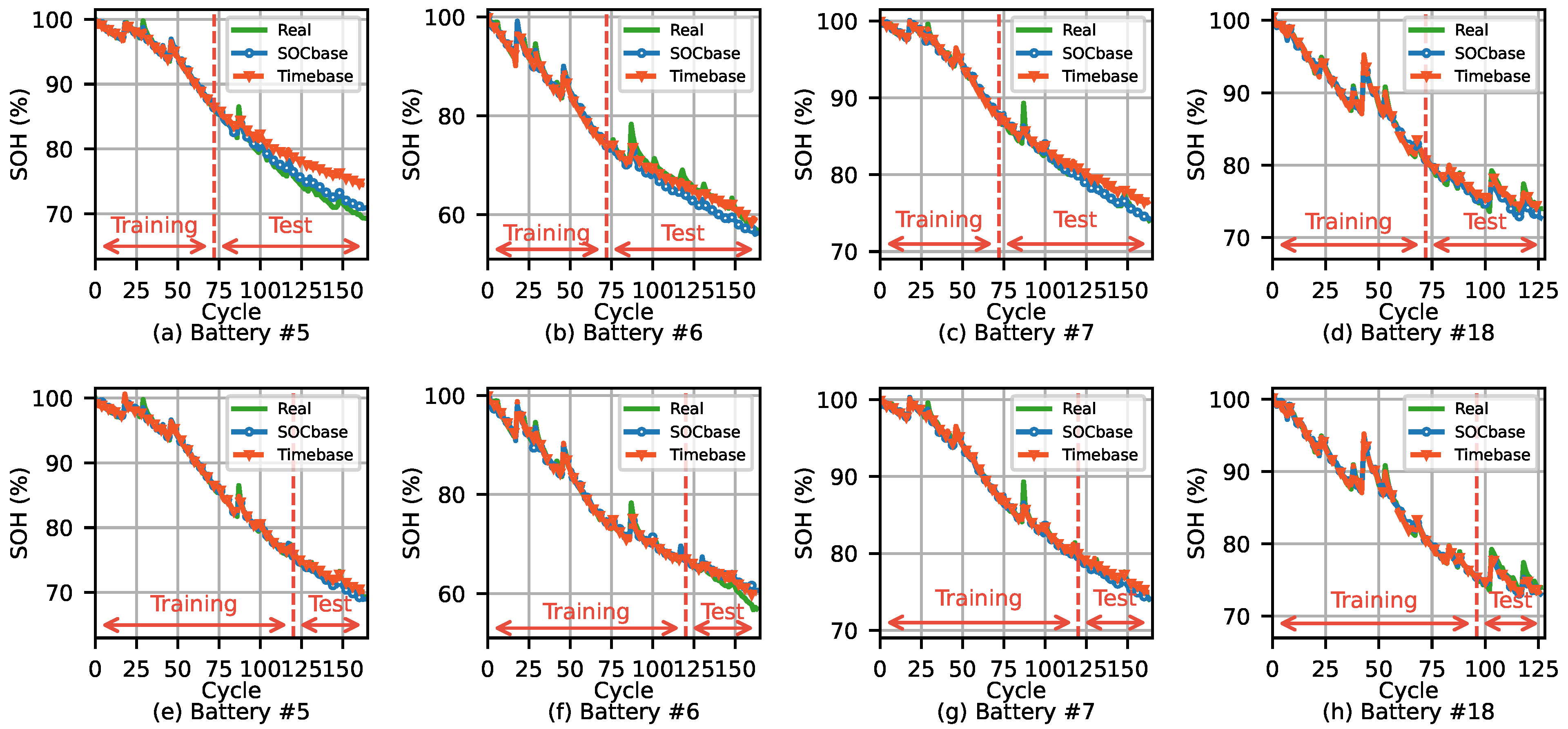
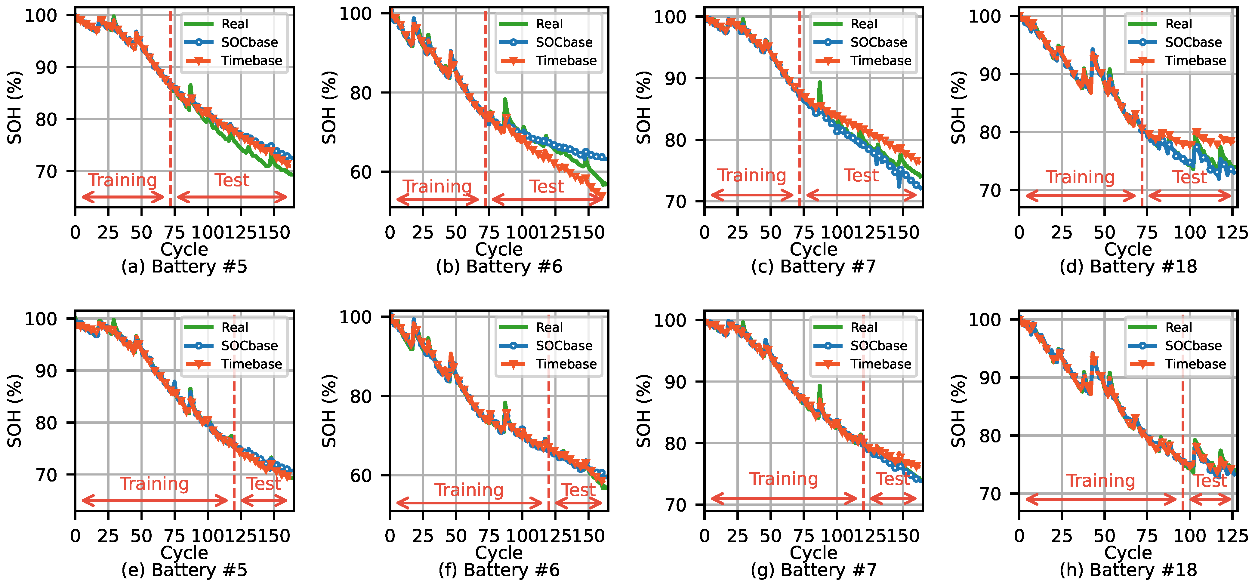
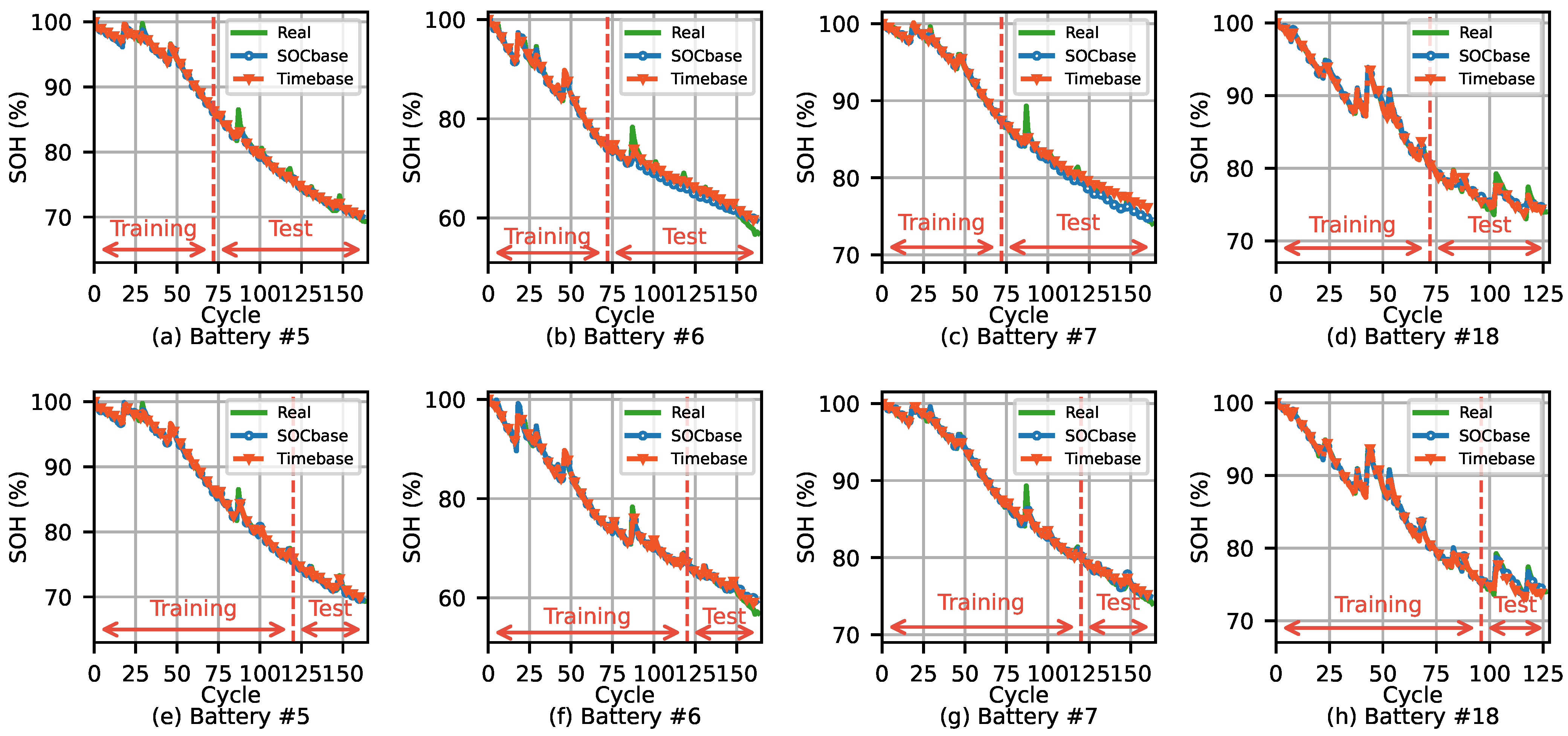
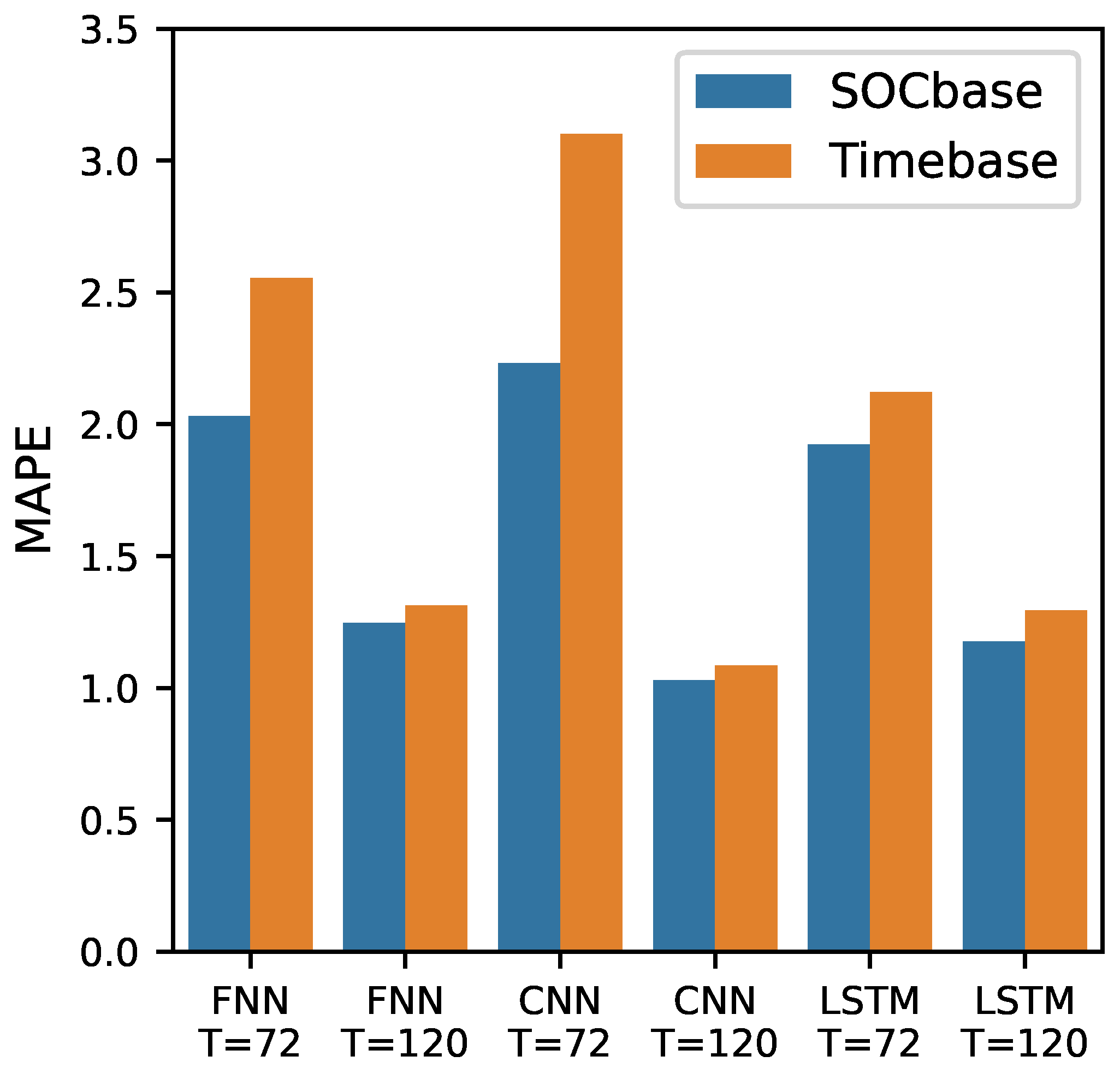
5.2. Estimation Results and Discussion

To validate the proposed method, the SOH estimation results of time-based sampling and SOC-based sampling were compared in this Section. To compare and infer which one performed better under limited training conditions, the SOH estimation was conducted in two cases: models trained with 72-cycle training and models trained with 120-cycle training without battery #18. In battery #18, one was a model trained with 72-cycle training, and the other was a model trained with 96-cycle training. In addition, all machine learning models were performed five times, and the average value of the results was used. Figure 6 shows SOH estimation results using the FNN in various batteries with 20 sampling points. The FNN with SOC-based datasets outperformed with the time-based datasets in 72-cycle training, as shown in Figure 6a–d. There was a significant difference in SOH estimation between SOC-based preprocessing and time-based preprocessing in SOH estimation results of Battery #5 and Battery #7, as shown in Figure 6a,c. However, the results of the two groups were similar on more training data, as shown in Figure 6e–h.

The SOH estimation results of the CNN showed a trend similar to those of the FNN, as shown in Figure 7. In 72-cycle training, the CNN with SOC-based datasets estimated the SOH more accurately than with the time-based datasets, as shown in Figure 7a–d. However, in 72-cycle training, the CNN with SOC-based datasets showed more errors than the FNN with SOC-based datasets. Similarly, the CNN with time-based datasets showed more errors than the FNN with time-based datasets. In the late stage, SOC-based and time-based datasets showed similar SOH estimation results in the CNN, as shown in Figure 7e–h.

However, the SOH estimation results for the LSTM differed slightly from those for the FNN. As shown in Figure 8a–d, the SOH was estimated similarly for both SOC-based and time-based datasets in 72-cycle training, and the LSTM had a higher estimation accuracy than FNN and CNN. In 120-cycle training, LSTM had a higher estimation accuracy in both SOC-based and time-based datasets. Because LSTM is an appropriate model for series-type data, these results were obtained.

To make a more straightforward comparison, we calculated the MAE, MASE, and MAPE of the SOH estimation, as shown in

Table 4. Estimation errors in various models and training cycles.

Model	Training	Processing	MAE	MSE	MAPE
FNN	72-Cycle	SOCbase	0.0396	0.0023	2.03
		Timebase	0.0611	0.0068	2.56
	120-Cycle	SOCbase	0.0225	0.0010	1.25
		Timebase	0.0253	0.0010	1.31
CNN	72-Cycle	SOCbase	0.0449	0.0040	2.23
		Timebase	0.0729	0.0131	3.10
	120-Cycle	SOCbase	0.0193	0.0008	1.03
		Timebase	0.0239	0.0011	1.09
LSTM	72-Cycle	SOCbase	0.0411	0.0039	1.92
		Timebase	0.0465	0.0042	2.12
	120-Cycle	SOCbase	0.0229	0.0009	1.18
		Timebase	0.0257	0.0011	1.29

. All the machine learning models showed a lower number of estimation errors on SOC-based datasets than on time-based datasets, as shown in Table 4. These results showed that the preprocessing based on the SOC was more suitable for machine learning than preprocessing based on the time intervals in the raw data of lithium-ion batteries.

The LSTM model trained using SOC-based datasets had the lowest MAPE of 1.92 among models trained with less data. However, even when a simple FNN model with SOC-based datasets was used, the MAPE showed the second lowest value at 2.03, which was lower than any model using time series data. Table 2 shows that the total number of parameters in FNN, CNN, and LSTM was 4081, 16,441, and 38,941, respectively. As a result, the total number of parameters in the FNN was only 25% of that in the CNN and 10% of that in the LSTM. On small training data, these results showed that FNN with SOC-based datasets outperformed complex models, such as CNNs and LSTMs. In models trained with large data, the CNN trained using SOC-based datasets had the lowest MAPE at 1.03. However, there was no significant difference in MAPE between SOC-based data processing and time-based data processing, as shown in Figure 9. The results of this study indicated that a simple FNN model with SOC-based data preprocessing could be used to predict the SOH accurately, similar to complex models, such as CNN and LSTM. Consequently, these results showed that the preprocessing method proposed in this study could improve the accuracy of the FNN model, which was 10% of the parameters of the LSTM model, as much as LSTM.

6. Conclusions

We proposed a new preprocessing method for machine learning models to improve the SOH estimation of batteries. The proposed preprocessing was based on the relative SOC, which could be easily calculated during charging using the current integration method. To compare the proposed method with the general preprocessing method based on constant time intervals, the correlation coefficient between datasets and usable capacities was calculated. The correlation results showed that SOC-based datasets processed using the proposed method had a higher correlation with usable capacity than general time-based datasets. Furthermore, we tested various machine learning models such as the FNN, CNN, and LSTM using SOC-based and time-based datasets. Our results showed that the simplest FNN model using the proposed method predicted the battery SOH with as much accuracy as complex models such as CNNs and LSTMs. Furthermore, the MAPE value of the FNN model with SOC-based datasets was 2.03, which was lower than 3.10 of the CNN model and 2.12 of LSTM model with time-based datasets tested on small training data. Our findings suggest that the proposed method could be used to improve the accuracy of devices with limited computing resources. Therefore, our findings can be applied to SOH estimation in resource-constrained hardware platforms. In future work, we intend to integrate the proposed method into embedded devices and apply it in tiny machine learning.

References

1. Whittingham, M.S. Electrical Energy Storage and Intercalation Chemistry. Science 1976, 192, 1126–1127. [Google Scholar] [CrossRef]
2. Stan, A.I.; Świerczyński, M.; Stroe, D.I.; Teodorescu, R.; Andreasen, S.J. Lithium Ion Battery Chemistries from Renewable Energy Storage to Automotive and Back-up Power Applications—An Overview. In Proceedings of the 2014 International Conference on Optimization of Electrical and Electronic Equipment (OPTIM), Bran, Romania, 22–24 May 2014; pp. 713–720. [Google Scholar]
3. Nishi, Y. Lithium Ion Secondary Batteries; Past 10 Years and the Future. J. Power Sources 2001, 100, 101–106. [Google Scholar] [CrossRef]
4. Huang, S.C.; Tseng, K.H.; Liang, J.W.; Chang, C.L.; Pecht, M.G. An Online SOC and SOH Estimation Model for Lithium-Ion Batteries. Energies 2017, 10, 512. [Google Scholar] [CrossRef]
5. Goodenough, J.B.; Kim, Y. Challenges for Rechargeable Li Batteries. Chem. Mater. 2010, 22, 587–603. [Google Scholar] [CrossRef]
6. Nitta, N.; Wu, F.; Lee, J.T.; Yushin, G. Li-Ion Battery Materials: Present and Future. Mater. Today 2015, 18, 252–264. [Google Scholar] [CrossRef]
7. Dai, H.; Jiang, B.; Hu, X.; Lin, X.; Wei, X.; Pecht, M. Advanced Battery Management Strategies for a Sustainable Energy Future: Multilayer Design Concepts and Research Trends. Renew. Sustain. Energ. Rev. 2021, 138, 110480. [Google Scholar] [CrossRef]
8. Lawder, M.T.; Suthar, B.; Northrop, P.W.; De, S.; Hoff, C.M.; Leitermann, O.; Crow, M.L.; Santhanagopalan, S.; Subramanian, V.R. Battery Energy Storage System (BESS) and Battery Management System (BMS) for Grid-Scale Applications. Proc. IEEE 2014, 102, 1014–1030. [Google Scholar] [CrossRef]
9. Zhang, L.; Fan, W.; Wang, Z.; Li, W.; Sauer, D.U. Battery Heating for Lithium-Ion Batteries Based on Multi-Stage Alternative Currents. J. Energy Storage 2020, 32, 101885. [Google Scholar] [CrossRef]
10. Jiang, B.; Dai, H.; Wei, X. Incremental Capacity Analysis Based Adaptive Capacity Estimation for Lithium-Ion Battery Considering Charging Condition. Appl. Energy 2020, 269, 115074. [Google Scholar] [CrossRef]
11. Tian, H.; Qin, P.; Li, K.; Zhao, Z. A Review of the State of Health for Lithium-Ion Batteries: Research Status and Suggestions. J. Cleaner Prod. 2020, 261, 120813. [Google Scholar] [CrossRef]
12. Onori, S.; Spagnol, P.; Marano, V.; Guezennec, Y.; Rizzoni, G. A New Life Estimation Method for Lithium-Ion Batteries in Plug-in Hybrid Electric Vehicles Applications. Int. J. Power Electron. 2012, 4, 302–319. [Google Scholar] [CrossRef]
13. Plett, G.L. Extended Kalman Filtering for Battery Management Systems of LiPB-Based HEV Battery Packs: Part 3. State and Parameter Estimation. J. Power Sources 2004, 134, 277–292. [Google Scholar] [CrossRef]
14. Goebel, K.; Saha, B.; Saxena, A.; Celaya, J.R.; Christophersen, J.P. Prognostics in Battery Health Management. IEEE Instrum. Meas. Mag 2008, 11, 33–40. [Google Scholar] [CrossRef]
15. Wang, D.; Yang, F.; Zhao, Y.; Tsui, K.L. Battery Remaining Useful Life Prediction at Different Discharge Rates. Microelectron. Reliab. 2017, 78, 212–219. [Google Scholar] [CrossRef]
16. Li, J.; Landers, R.G.; Park, J. A Comprehensive Single-Particle-Degradation Model for Battery State-of-Health Prediction. J. Power Sources 2020, 456, 227950. [Google Scholar] [CrossRef]
17. Wang, Q.; Wang, Z.; Zhang, L.; Liu, P.; Zhang, Z. A Novel Consistency Evaluation Method for Series-Connected Battery Systems Based on Real-World Operation Data. IEEE Trans. Transport. Electrific. 2020, 7, 437–451. [Google Scholar] [CrossRef]
18. Ren, L.; Zhao, L.; Hong, S.; Zhao, S.; Wang, H.; Zhang, L. Remaining Useful Life Prediction for Lithium-Ion Battery: A Deep Learning Approach. IEEE Access 2018, 6, 50587–50598. [Google Scholar] [CrossRef]
19. Hu, X.; Jiang, J.; Cao, D.; Egardt, B. Battery Health Prognosis for Electric Vehicles Using Sample Entropy and Sparse Bayesian Predictive Modeling. IEEE Trans. Ind. Electron. 2015, 63, 2645–2656. [Google Scholar] [CrossRef]
20. Piao, C.; Li, Z.; Lu, S.; Jin, Z.; Cho, C. Analysis of Real-Time Estimation Method Based on Hidden Markov Models for Battery System States of Health. J. Power Electron. 2016, 16, 217–226. [Google Scholar] [CrossRef] [Green Version]
21. Liu, D.; Pang, J.; Zhou, J.; Peng, Y.; Pecht, M. Prognostics for State of Health Estimation of Lithium-Ion Batteries Based on Combination Gaussian Process Functional Regression. Microelectron. Reliab. 2013, 53, 832–839. [Google Scholar] [CrossRef]
22. Liu, D.; Zhou, J.; Pan, D.; Peng, Y.; Peng, X. Lithium-Ion Battery Remaining Useful Life Estimation with an Optimized Relevance Vector Machine Algorithm with Incremental Learning. Measurement 2015, 63, 143–151. [Google Scholar] [CrossRef]
23. Jia, J.; Liang, J.; Shi, Y.; Wen, J.; Pang, X.; Zeng, J. SOH and RUL Prediction of Lithium-Ion Batteries Based on Gaussian Process Regression with Indirect Health Indicators. Energies 2020, 13, 375. [Google Scholar] [CrossRef] [Green Version]
24. Patil, M.A.; Tagade, P.; Hariharan, K.S.; Kolake, S.M.; Song, T.; Yeo, T.; Doo, S. A Novel Multistage Support Vector Machine Based Approach for Li Ion Battery Remaining Useful Life Estimation. Appl. Energy 2015, 159, 285–297. [Google Scholar] [CrossRef]
25. Khumprom, P.; Yodo, N. A Data-Driven Predictive Prognostic Model for Lithium-Ion Batteries Based on a Deep Learning Algorithm. Energies 2019, 12, 660. [Google Scholar] [CrossRef] [Green Version]
26. Xia, Z.; Qahouq, J.A.A. Adaptive and Fast State of Health Estimation Method for Lithium-Ion Batteries Using Online Complex Impedance and Artificial Neural Network. In Proceedings of the 2019 IEEE Applied Power Electronics Conference and Exposition (APEC), Anaheim, CA, USA, 17–21 March 2019; pp. 3361–3365. [Google Scholar]
27. She, C.; Wang, Z.; Sun, F.; Liu, P.; Zhang, L. Battery Aging Assessment for Real-World Electric Buses Based on Incremental Capacity Analysis and Radial Basis Function Neural Network. IEEE Trans. Ind. Informat. 2019, 16, 3345–3354. [Google Scholar] [CrossRef]
28. Eddahech, A.; Briat, O.; Bertrand, N.; Delétage, J.Y.; Vinassa, J.M. Behavior and State-of-Health Monitoring of Li-Ion Batteries Using Impedance Spectroscopy and Recurrent Neural Networks. Int. J. Electr. Power Energy Syst. 2012, 42, 487–494. [Google Scholar] [CrossRef]
29. Tian, J.; Xiong, R.; Shen, W.; Lu, J.; Yang, X.G. Deep Neural Network Battery Charging Curve Prediction Using 30 Points Collected in 10 Min. Joule 2021, 5, 1521–1534. [Google Scholar] [CrossRef]
30. Shen, S.; Sadoughi, M.; Chen, X.; Hong, M.; Hu, C. A Deep Learning Method for Online Capacity Estimation of Lithium-Ion Batteries. J. Energy Storage 2019, 25, 100817. [Google Scholar] [CrossRef]
31. Park, K.; Choi, Y.; Choi, W.J.; Ryu, H.Y.; Kim, H. LSTM-Based Battery Remaining Useful Life Prediction with Multi-Channel Charging Profiles. IEEE Access 2020, 8, 20786–20798. [Google Scholar] [CrossRef]
32. Saha, B.; Goebel, K. Battery Data Set, NASA Ames Prognostics Data Repository; NASA Ames Research Center: Moffett Field, CA, USA, 2007. Available online: https://ti.arc.nasa.gov/tech/dash/groups/pcoe/prognostic-data-repository/ (accessed on 25 September 2020).
33. Choi, Y.; Ryu, S.; Park, K.; Kim, H. Machine Learning-Based Lithium-Ion Battery Capacity Estimation Exploiting Multi-Channel Charging Profiles. IEEE Access 2019, 7, 75143–75152. [Google Scholar] [CrossRef]
34. Le, D.; Tang, X. Lithium-Ion Battery State of Health Estimation Using Ah-V Characterization. In Proceedings of the Annual Conference of the PHM Society, Montreal, QC, Canada, 25–29 September 2011; p. 1. [Google Scholar] [CrossRef]
35. Kim, I.S. A Technique for Estimating the State of Health of Lithium Batteries through a Dual-Sliding-Mode Observer. IEEE Trans. Power Electron. 2009, 25, 1013–1022. [Google Scholar]
36. Ng, K.S.; Moo, C.S.; Chen, Y.P.; Hsieh, Y.C. Enhanced Coulomb Counting Method for Estimating State-of-Charge and State-of-Health of Lithium-Ion Batteries. Appl. Energy 2009, 86, 1506–1511. [Google Scholar] [CrossRef]
37. Zhang, J.; Lee, J. A Review on Prognostics and Health Monitoring of Li-Ion Battery. J. Power Sources 2011, 196, 6007–6014. [Google Scholar] [CrossRef]
38. Kirchev, A. Electrochemical Energy Storage for Renewable Sources and Grid Balancing; Elsevier: Amsterdam, The Netherlands, 2015; pp. 411–435. [Google Scholar]
39. Crocioni, G.; Pau, D.; Delorme, J.M.; Gruosso, G. Li-Ion Batteries Parameter Estimation with Tiny Neural Networks Embedded on Intelligent IoT Microcontrollers. IEEE Access 2020, 8, 122135–122146. [Google Scholar] [CrossRef]
40. Casari, A.; Zheng, A. Feature Engineering for Machine Learning; O’Reilly Media: Sebastopol, CA, USA, 2018. [Google Scholar]
41. Loshchilov, I.; Hutter, F. Decoupled Weight Decay Regularization. arXiv 2017, arXiv:1711.05101. [Google Scholar]
42. Goodfellow, I.; Bengio, Y.; Courville, A. Deep Learning; MIT Press: Cambridge, MA, USA, 2016. [Google Scholar]
43. Hochreiter, S.; Schmidhuber, J. Long Short-Term Memory. Neural Comput. 1997, 9, 1735–1780. [Google Scholar] [CrossRef] [PubMed]
Figure 1. Lithium-ion battery degradation with respect to number of cycles.
Energies 14 07206 g001
Figure 2. Data sampled by constant time intervals during charging of battery #5.
Energies 14 07206 g002
Figure 3. Data sampled by constant SOC intervals during charging of battery #5.
Energies 14 07206 g003
Figure 4. Heatmap of the Pearson correlation coefficient for the data processing method between the usable capacity of the battery and the sample data of current, voltage, and temperature difference during charging.
Energies 14 07206 g004
Figure 5. Overview of the proposed process for battery capacity estimation.
Energies 14 07206 g005
Figure 6. SOH estimation results using FNN.
Energies 14 07206 g006
Figure 7. SOH estimation results using a CNN.
Energies 14 07206 g007
Figure 8. SOH estimation results using LSTM.
Energies 14 07206 g008
Figure 9. MAPE in various models and training cycles.
Energies 14 07206 g009