Abstract
As renewable energy increasingly penetrates into electricity-heat integrated energy system (IES), the severe challenges arise for system reliability under uncertain generations. A two-stage approach consisting of pre-scheduling and re-dispatching coordination is introduced for IES under wind power uncertainty. In pre-scheduling coordination framework, with the forecasted wind power, the robust and economic generations and reserves are optimized. In re-dispatching, the coordination of electric generators and combined heat and power (CHP) unit, constrained by the pre-scheduled results, are implemented to absorb the uncertain wind power prediction error. The dynamics of building and heat network is modeled to characterize their inherent thermal storage capability, being utilized in enhancing the flexibility and improving the economics of IES operation; accordingly, the multi-timescale of heating and electric networks is considered in pre-scheduling and re-dispatching coordination. In simulations, it is shown that the approach could improve the economics and robustness of IES under wind power uncertainty by taking advantage of thermal storage properties of building and heat network, and the reserves of electricity and heat are discussed when generators have different inertia constants and ramping rates.
1. Introduction
With the enhancement of coupling between multi-type energy sources, integrated energy system (IES) has drawn the increasing attention. In IES, combined heat and power (CHP) unit, as a significant component, generates electricity and heat simultaneously, leading to the higher energy utilization efficiency. With the growth in utilization of CHP unit, its heat-led mode has caused serious wind abandonment especially in winter heating periods. This becomes a key issue limiting wind power penetration. Moreover, the strong intermittency and uncertainty of wind power make its precise forecasting difficult to achieve; as a result, the current wind power prediction error is usually up to 25% to 40% [1], imposing serious challenges to the secure and stable operation of IES.
Many studies have been conducted to improve the flexibility of electricity and heat coupled IES under wind power uncertainty. The maximum flexibility of a combined heat and power system with thermal energy storage is discussed [2], where the robustness of the system under renewable energy resources uncertainty is not considered. A chance-constrained programming-based scheduling is proposed [3], with the joint operation optimization of battery energy storage and heat storage tank integrated. However, the distribution of uncertainty is assumed to be known, which is inconsistent with engineering practice. Two-stage scheduling is a commonly used approach to deal with wind power uncertainty. The two stages are implemented day-ahead and in real time, based on day-ahead wind power prediction and wind power realization, respectively. In the first pre-scheduling stage, the factors such as units’ startup and shutdown, heat storage tank capacity, etc. need to be determined in advance. Furthermore, in the second stage, namely re-dispatching, the decision should be amended to compensate for wind prediction error, such as units’ generations and so on. In [4], a minimax regret model based two-stage robust scheduling for IES is introduced, where the electrical and thermal load tracking strategies are applied to attenuate the uncertainty. However, its heat balance cannot be guaranteed under wind power uncertainty. A two-stage robust operation strategy is explored [5]. The decisions of day-ahead thermal storage charging/discharging are in the first stage, and the decisions of CCHP and auxiliary boiler output are in the second stage to compensate the first stage operation and follow the uncertainty realization. However, its timescale for the second-stage is too long. The real-time robustness of the system cannot be guaranteed due to the randomness of wind power changes. A scenario-based stochastic multi-energy scheduling is developed in [6], where the scenario-independent and scenario-relative two-stage decisions are made in an optimization model with various energy storage considered. However, of all the mentioned research above, the energy storage units are installed to alleviate uncertain wind power, which is not recommended since it might cause extra costs and failures. Taking full advantage of thermal energy storage of heating system can solve this problem.
Distinct from electric system, heat energy supply and demand balance are kept not instantaneously but during a period, since a few minutes to several hours are taken for hot water to carry heat energy from source to load through pipeline [7]. Moreover, the real-time heat power imbalance is reflected in the variation of water temperature, the operational limits of which are within a wider range. Thus, contrary to the electric transmission network, the heat network could serve as a natural thermal storage, bringing great flexibility to wind power absorption in IES. Several scholars have noticed the potential role of heat network and endeavored to implement coordinated scheduling by considering the dynamics of thermal energy transmission. The unit commitment in IES is studied [8], where temperature quasi-dynamics of heat network is modeled to characterize its heat storage capacity in CF-VT (constant mass flow and variable temperature) strategy. The intra-day power dispatching of IES is explored [7], integrating the heat network dynamics under the variable mass flow and variable temperature (VF-VT) strategy. A dispatching model of IES is proposed, considering thermal energy storage of pipelines and the detailed heat transfer constraints [9].
Furthermore, the heat load at an instant is usually pre-given as a constant in previous research on heat and electricity coupled scheduling. However, since the building has the potential of thermal energy storage and could offer a source of flexibility to absorb wind power, it is necessary to model the heat load and then integrate it into the coordinated scheduling. The storage capacity of building could be illustrated as follows: similar to heat network, the thermal inertia of building is reflected in thermal transmission dynamics, usually lasting for a period that could not be ignored. In building, the instantaneous imbalance between heat power supply and demand is allowed, resulting in indoor temperature changes; and the indoor temperature meeting human comfort requirements is usually given as an interval. In addition, modeling the building’s heat load by considering the heat loss and comfortable requirement for indoor temperature could improve the practicality of the approach. In a few studies on heat and electricity coupled scheduling, the dynamic heat load model of buildings is established. Feasible region method is proposed to formulate the flexibility of IES [10] and the IES scheduling with demand response is explored [11], where the first-order equivalent thermal parameter method is employed to model the heat dissipation of building. The thermal modeling of dwelling is established through equivalent thermal resistance and capacitance, and the expected thermal discomfort metric is defined to quantify user’s discomfort level [12].
In order to accommodate uncertain wind power in two stages of pre-scheduling with its forecasting value and re-dispatching with its uncertain realization, a two-stage robust and economical scheduling methodology of IES is developed. In this method, the natural storage capacity of heat network and buildings, and the reserves and generations of electric generators and CHP unit are utilized. The main contributions of the paper are summarized as follows:
- The dynamic models of heat network and building are established to describe their thermal energy storage characteristics. Their storage capacities are utilized and integrated in the two-stage robust and economic scheduling to accommodate wind power. The thermal transmission dynamics in the seat network represents the water temperature variations with respect to time variable and pipeline position, considering heat loss, heat propagation and time-delay of flowing. In order to make a practical description of the thermal demand from building, the heat dissipation process from indoor to outdoor is modeled, and the standard effective temperature (SET) is applied to measure the degree of user’s thermal comfort.
- Inspired by the robust scheduling of power system [13], the approach for accommodating uncertain wind power in heat and electricity coupled IES is developed, specifically in two stages, i.e., in pre-scheduling with its forecasted value and in re-dispatching with its realization, by utilizing the coupled reserves of electricity generators and co-generator CHP unit, along with the natural thermal storage of heat network and building. With the predicted wind power, the robust generation and reserves of electric generators and CHP unit are optimized in pre-scheduling, where the dynamics of building and heat network are integrated to absorb wind power. With the uncertain realization of wind power, prediction error is alleviated in re-dispatching constrained by the reserves optimized in pre-scheduling. In pre-scheduling, the feasibility constraints of re-dispatching solution under uncertain realization are considered, with zero-sum game between the re-dispatching and wind power uncertainty formulated as a max–min problem.
- In the electricity-heat IES, the generators with different inertia constants and reserve costs are considered, leading to two situations: the reserve supply by CHP unit or not. Due to the strong coupling between electricity supply and heat provision of CHP unit, when the CHP generator takes on the electricity reserve, there exists the security margins of temperature in heat network and building to provide heat reserve. From this perspective, the natural energy storage capacity of heat pipeline and building could be utilized to serve as heat reserve in electricity-heat coupled IES. When no reserve is required from CHP unit due to its high cost, the temperatures in heat network and building could reach their bounds, induced by the objective of economic operation.
The remainder of this paper is organized as follows. Section 2 describes the framework of two-stage robust economic scheduling approach. In Section 3, the detailed formulations of robust economic scheduling problem in electricity-heat coupled IES are illustrated, where the heat transmission dynamics in heat network and building are modeled. Simulation results are presented in Section 4 to demonstrate the effectiveness of the proposed approach. Conclusions are finally given in Section 5.
2. Framework Description
2.1. Uncertainty Set
In robust and economic scheduling, uncertainty set is used to define the possible range of uncertain variables. Excessive description of uncertainty may lead to conservatism, i.e., higher operational cost; while insufficient consideration of uncertainty cannot guarantee the operational reliability under uncertain realizations. Since it is almost impossible for all the predicted values simultaneously reaching the boundaries, budget uncertainty set is adopted to describe and restrict wind power uncertainty [13], formulated as:
where is the uncertainty set of wind power; is the wind power at time ; and are the upper and lower bounds of prediction interval; the uncertainty budge is the number of uncertainty variables reaching the boundaries, influencing the conservativeness. According to the central limit theorem, the value of is given as [13]
where and are the expected value and standard deviation of ; is the number of uncertain variables; is the cumulative probability distribution function of standard normal distribution; is the confidence level. All the parameters in (1)–(3) can be obtained by the historical and predicted values of wind power.
2.2. Coordinated Framework and Multi-Timescale
To alleviate wind power uncertainty, before and after the real value of wind power is observed, the scheduling is divided into two stages, i.e., pre-scheduling and re-dispatching, the framework of which is displayed in Figure 1. In pre-scheduling stage, the robust and economic generations and reserves of electric generators and CHP unit are optimized based on the predicted wind power, where the robust feasibility constraint is considered. In re-dispatching stage, with the wind power realization, the coordinated generations of electric generators and CHP unit are optimized within the pre-scheduled reserves to compensate the wind power forecasting error. In the pre-scheduling and re-dispatching, the optimization is implemented over a time window rather than just at an instant in order to describe the thermal dynamics. In the proposed approach, two kinds of generators are included, the CHP unit and electricity generator that only generates electric power.
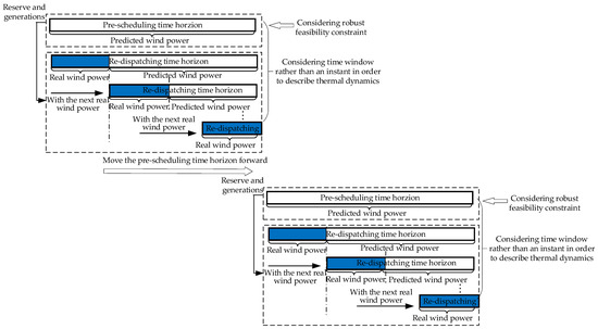
Figure 1.
Coordinated framework of pre-scheduling and re-dispatching.
The pre-scheduling problem is formulated as (4) [13]:
where is the cost coefficient vector; represents the constraints for economic operation; is the predictive wind power; denotes the feasible region of re-dispatching strategy, which is a function of the uncertain wind power realization and pre-scheduling decision ; the uncertain set of wind power is defined as , determined by (1)–(3). In order to ensure the secure operation of IES under the uncertain wind power prediction error, the pre-scheduling strategy , composed by the optimal coordinated generations and reserves of electric generators and CHP unit, needs to ensure that there exists a feasible re-dispatching strategy for any under the pre-scheduled reserves. Insufficient reserves may lead to the infeasibility of re-dispatching and drive the system to an unsecure operating state. On the contrary, excessive reserves may result in higher operational cost. Therefore, as shown in pre-scheduling problem (4), gives the constraint that the appropriate reserves should satisfy. The detailed formulation of will be illustrated in Section 2.3, where zero-sum game describes the relation between uncertain wind power realization and re-dispatching.
The re-dispatching optimization can be expressed as:
As shown in Figure 1, in the re-dispatching time horizon, considering that the current dispatching strategy may have some impact on the subsequent operation states of IES because of the long transient process of heat network, not only the real wind power at the current moment but the predicted values at following instants are used, denoted as in (5). Among the re-dispatched strategies over the time horizon, only the current one is implemented on the IES.
In the pre-scheduling and re-dispatching of electricity-heat coupled IES, two timescales are considered for electricity and heat networks coordinate in the unified framework, shown in Figure 2 and Figure 3. It is assumed that the time resolution of wind power prediction is . The smaller time resolution of real wind power fluctuation is defined as . The inertia of CHP unit is assumed to be smaller and the time resolution of ramping up/ down is set as . The electricity generators having different inertia are considered, respectively with the different ramping time resolution and .
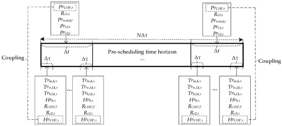
Figure 2.
Multi-timescale coordination in pre-scheduling.
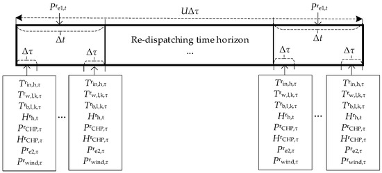
Figure 3.
Multi-timescale coordination in re-dispatching.
In pre-scheduling, the timescale of the variables in power grid, such as the electricity power of CHP unit and electric generators, is same as that of the predicted wind power; the timescale of the variables in heat network is , such as the heating power by CHP unit, the temperatures of flowing water and insulation layer, heat load, indoor temperature and so on; the timescale of the reserves from CHP unit and the electric generator with smaller inertia is and that of the reserves from the electric generator with larger inertia is . In re-dispatching, the time resolution of real wind power is ; the timescale of the generations from CHP unit and the electric generator with smaller inertia is since they are dispatched to follow wind power fluctuation, while that of the power of the electric generator with larger inertia is because of its slower ramping rate.
2.3. Robust Feasibility Constraint of Re-Dispatching in Pre-Scheduling
In pre-scheduling, besides the electricity and heat power generations, the optimal reserves of electric generators and CHP unit are derived to ensure the feasibility of re-dispatching under uncertain wind power, while both economy and robustness are guaranteed. The dispatcher and the uncertain wind power act as the two sides of zero-sum game [13], i.e., uncertainty intends to violate the secure constrains of the system as much as possible, resulting in more reserve required; on the contrary, facing the uncertainty, the dispatcher tries to maintain secure operation through dispatching strategy constrained by the reserve, which is expected as low as possible due to the objective of economic operation.
With a given pre-scheduling strategy , the indicator is formulated in (6) to reflect the feasibility of re-dispatching strategy under wind power realization [13].
where and are the introduced slack variables. If re-dispatching is feasible, there must exist a solution where ; on the contrary, if re-dispatching is unfeasible, .
The most unfavorable wind power realization intends to maximize , and the zero-sum game between the dispatcher and wind power uncertainty is expressed as
With the pre-scheduling strategy , suggests that there exists the feasible re-dispatching strategy under any wind power realization ; indicates that the most unfavorable wind power realization could make re-dispatching problem infeasible. By transforming the inner layer into its dual problem, the problem in (7) can be converted into a single-layer optimization:
where is dual variable. The optimization (8) is a mixed integer programming problem containing quadratic form in its objective function. It can be solved by many solvers such as Cplex.
Up to now, it is almost impossible to give the explicit expression of constraint . However, with the solution of (8), the iterative solving approach of pre-scheduling strategy is proposed to guarantee its robust feasibility [13], illustrated as follows:
is linearly approximated at
where is the optimal solution of (8). Then, the robust feasible should satisfy the constraint.
In order to replace , constraint (10) is gradually added to the optimization problem (8) until . Then a robust feasible solution can be derived.
2.4. Procedure of Two-Stage Robust Economic Scheduling
The procedure of two-stage robust economic scheduling is illustrated as follows.
Step 1. Set initial parameter , , , , where denotes the iterative step;
Step 2. The pre-scheduling problem (4) is solved, where the robust feasible constraint is replaced by the constraints , ; and then .
Step 3. With the obtained pre-scheduling strategy , calculate according to (8). If , the pre-scheduling ends and the re-dispatching in (5) is optimized with the real wind power; otherwise, derive the constraint where , , and go to Step 2.
3. Model Formulation
3.1. Pre-Scheduling Model
3.1.1. Optimization Objective
The optimization objective in pre-scheduling is to minimize the total costs during the time horizon, including the costs for operations and reserves of CHP unit and electric generators. It is formulated as:
3.1.2. Optimization Constraints
- (1)
- CHP unitThere are usually two types of CHP units, back-pressure turbine and extraction condensing turbine [14]. For the former, the heat-to-electricity ratio is constant and the relation between electricity and heat power is linear; for the latter, the heat-to-electricity ratio varies in a wide range by pumping rate, with the lower energy efficiency and more flexibility compared with the former. In the paper, in order to show the flexibility brought by thermal storage of heat network and building, the CHP unit with the fixed heat-to-electricity ratio is chosen to study. Its operational characteristics is described as:as shown in (12), the CHP unit combines the different timescale and .CHP unit generation is constrained by the ramping rate in MW/. Since the timescale of CHP unit generated electric power is in pre-scheduling, its ramping rate constraint is described as:The scheduled electric power output of CHP is bounded by its upper and lower limits considering reserve:The scheduled reserve cannot exceed its upper limit:
- (2)
- Electricity networkFor electric network modeling, DC power flow model is employed for simplicity. The active power flow through bus to bus is described aswhere is the reactance of line from to ; and are the voltage phase angle at bus and at the time respectively.For each bus , power balance constraint should be satisfiedwhere and are power injection and load at bus at time respectively; denotes the set of buses directly connected with bus ; active flow is the active power though the line between bus and , which is positive when inflow to bus and negative when outflow from bus .Moreover, a slack node is defined, whose voltage phase angle remains zero:The voltage phase angle at a bus should be kept within its upper and lower limits:The power flow is limited by its transmission line capacity:Similar to CHP unit, the output of electric generators is also constrained by the ramping rate and the upper and lower bounds:The reserve should also be kept in its physical limit:
- (3)
- Heat networkHeat network is mainly composed of heat exchanger stations, pipelines and loads. Heat energy is extracted from the heat station, carried by hot water and distributed to heat consumers through heat pipelines. Heat transfer time, usually varying from hours to days, cannot be ignored [7]. In the paper, the thermal transmission dynamics of heat network is described since steady thermal model cannot reflect its energy storage property. The pressure dynamics are faster than thermal dynamics, with little impact on temperature distribution, so it is not considered here.
- (a)
- Heat pipelineFor a pipeline, in radial direction, hot water dissipates heat energy to insulation and the surrounding soil; while in axial direction, hot water transfers heat energy downwards through water flowing. Consequently, the water temperature in the pipeline varies with the time τ and the position variable x along the pipeline, representing its temporal and spatial characteristics. The most commonly used strategy CF-VT in north China is considered.The pipeline is divided equally into small segments of length . For the segment k, the thermal transmission dynamical model is established by including the heat dissipation to the surrounding soil and heat transferring to the adjacent segment, and then the heat energy delivering dynamics through the pipeline is modelled considering the pipeline topology.The thermal resistance between hot water and insulation layer can be calculatedThe thermal resistance between insulation layer and soil layer can be described asThe insulation layer absorbs heat energy from the hot water and then dissipates it to the soil layer. The heat dissipation of the insulation layer can be expressed aswhere .In additional to the heat energy dissipation to insulation layer, heat energy is transferred to the adjacent next segment at the same time, which is modeled asUsing the finite difference approximation method, (30) can be reformulated asThe water temperature is limited by the upper and lower bounds
- (b)
- HydraulicsIn order to model the hydraulics of the pipeline, the following assumptions are made: (1) Water is continuous and uncompressible, and according to mass conservation law, the mass flow entering into a node is equal to the mass flow leaving the node; (2) there is no heat energy loss at the mixed node; (3) when the flowing water meets at the crossing node, the water temperature uniformly mixes instantly.The mass flow balance at the mixed node is expressed aswhere and are the sets of pipelines that flows into and out of node .At the crossing node , the water temperature after mixing is given as
- (c)
- Heat exchangerAbsorbing the heat energy produced by CHP unit, the heat exchanger heats the water at the terminal end of return pipeline, which then flows out of the exchanger to the beginning end of supply pipeline. The heat exchange station is simplified to a node r, and the heat energy exchange is formulated aswhere is the heat energy utilization coefficient of heat exchanger.
- (d)
- Heat loadThe heat load refers to the heat power which is absorbed from the heat network to maintain the temperature of the building within the human comfort range, while the heat dissipation from the building interior to exterior is considered.Similar to the heat exchange station, the heat load is simplified to be a node g. It absorbs heat energy from the hot water flowing in supply network. The heat exchange at the heat load is expressed asDue to the difference between indoor and outdoor temperature, the heat power dissipates from indoors to outdoors. It is assumed that the heat dissipation power is linearly proportional to the temperature difference, which is formulated aswhere the heat transfer coefficient of building is related to the structure of the fences such as windows and walls; the outdoor temperature of building at time in pre-scheduling is a known parameter.Considering the heat energy absorption from the heat network and the heat energy dissipation from indoors to outdoors, the indoor temperature of the building can be expressed asThe indoor temperature should be restricted within a certain range in order to guarantee thermal comfort of users. SET established by the ASHRAE (American Society of Heating, Refrigerating and Air-Conditioning Engineers) is introduced in the paper for its universality and concision. The range of comfortable indoor temperature has the following constraints [15]:
3.2. Re-Dispatching
3.2.1. Optimization Objective
The optimization objective of re-dispatching is to minimize the total operational costs of CHP unit and electric generators during the time horizon, formulated as:
3.2.2. Optimization Constraints
With the pre-scheduled reserve, the outputs of generators are appropriately adjusted to adapt to the wind power realization in re-dispatching. Similar to Section 3.2, the operational constraints of re-dispatching are illustrated below.
CHP unit constraints are given in (41)–(43):
Electricity network constraints are represented in (44)–(52):
The heat network constraints in (27)–(29), (31)–(39) are included in re-dispatching optimization, with the superscript ‘p’ replaced by ‘r’.
4. Simulation Results
To illustrate the effectiveness of the two-stage robust and economic scheduling methodology for electricity and heat coupled IES in accommodating uncertain wind power, an electricity-heat IES, with an IEEE 9-bus, 9-branch electricity network and a 3-building, 12-pipeline heat network, is established in Figure 4. The two electricity and heat networks are coupled by CHP unit and heat exchanger. Electricity generator G1 with larger inertial time constant is attached to Bus 1, and the electricity generator G2 with smaller inertial time constant is installed at Bus 7. The parameters involved in the simulation are given in Table A1.
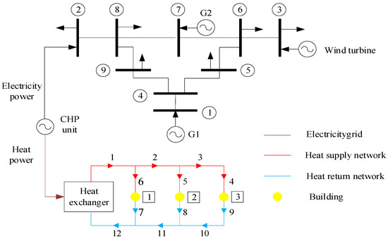
Figure 4.
Diagram of electricity-heat IES.
Several cases are implemented to explore the effectiveness of thermal energy storage properties of buildings and heat network in improving system flexibility and enhancing wind power absorption. The cases with different considered factors, such as storage capacity of heat network and buildings, time-of-use price of CHP unit generation, ramping speed limit of generators, are listed in Table 1, where √ denotes considering the factor while × denotes not. In Cases I, II and IV, the cost coefficients remain unchanged during the scheduling; while the cost coefficient of CHP generation varies in Case III, as shown in Table 2. The real and forecasted wind power values are depicted in Figure A1. The electricity load and outside temperature are drawn in Figure A2 and Figure A3.

Table 1.
Simulation cases and the considered factors.
Table 2.
Cost coefficients of generators.
4.1. Case I
From Figure A2 and Figure A3, it can be observed that during the scheduling horizon, the thermal demand gradually increases as the outdoor temperature drops; on the contrary, the electrical load gradually decreases. The pre-scheduled electricity generations and the balance between electricity supply and demand are depicted in Figure 5. The water temperature of heat network is drawn in Figure 6. It can be seen, in order to achieve economic operation, the generator G1 with the cheapest cost coefficient is scheduled to generate the most electric power; the G2 generation is very small in order to satisfy the down reserve requirement; the CHP unit with the highest cost coefficient is scheduled to satisfy the heat demand by the lowest generation, which can be indicated by the phenomenon shown in Figure 6 that the water temperature at the return Pipeline 7 at the end of the pre-scheduling period is close to its lower limit.
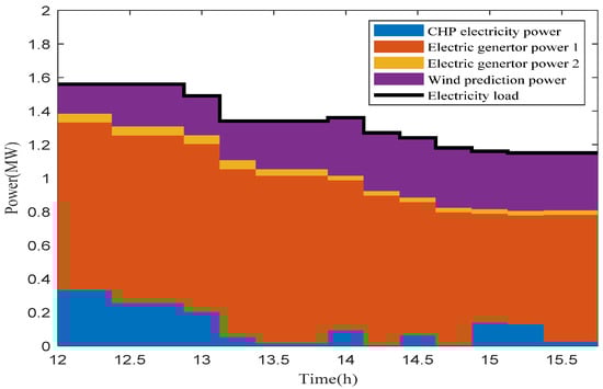
Figure 5.
Pre-scheduled electricity generations and the balance between supply and demand in Case I.
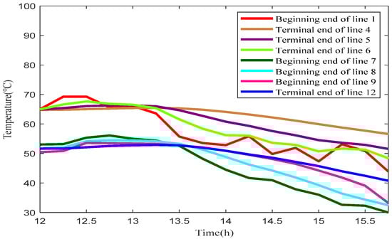
Figure 6.
Pre-scheduled water temperatures in heat network in Case I.
The temperature at the beginning of Line 1, i.e., the outlet of heat station, fluctuates greatly, for it is closely related with CHP unit generation. In order to maintain the real-time supply and demand balance of electricity load, the heat power output of CHP unit with the fixed heat-to-electricity ratio has a higher volatility. However, after the heat transferring through the pipelines, the temperature curves at the inlet of the load and the heat station, such as the beginning of Lines 4–6 and 12, becomes smooth. Consequently, from this perspective, the large volume of water in the pipeline serves as energy storage and the fluctuation of instantaneous load or wind power can be smoothed by heat network.
The imbalance between heat supply and demand is depicted in Figure 7. From 12:00 to 13:00, CHP unit generates more heat power than the total building dissipation. Further, the surplus heat energy, depicted in green, is stored into the pipeline and buildings. From 13:00 to 16:00, since the electricity demand decreases and at the same time the heat load increases, the stored heat energy drawn in yellow, is discharged to satisfy the heat demand, ensuring the indoor temperature in comfortable range. The indoor temperatures of buildings are shown in Figure 8.

Figure 7.
Pre-scheduled heat energy charging and discharging in Case I.
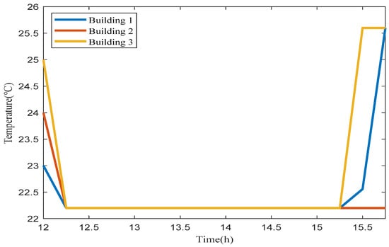
Figure 8.
Pre-scheduled building indoor temperature in Case I.
Due to predicted wind power errors, CHP unit and electric generators need to keep some reserve in advance. If the robust and economical scheduling methodology is not considered, when there is wind power prediction error, the system cannot meet the electric and heat balance for lack of reserve, which leads to infeasibility. On the contrary, when robust and economical scheduling methodology is taken into consideration, the system can operate safely and stably and also absorb all wind power. The costs are manifested in Table 3.
Table 3.
Comparison of reserve and operation cost between Cases I and II.
The reserves of generators are shown in Figure 9. At each instant, the sum of the electricity power reserves of all generators is 0.03 MW, equal to the wind power uncertainty. It is worth noting that the reserve of G1 is always 0. It is because that the timescale △t of G1 ramping speed is larger than the time resolution △τ of wind power fluctuation. In order to achieve economic operation, G2 with the cheaper reserve cost should be given more priority to provide reserve, rather than CHP unit. CHP unit will take on the remaining reserve when G2 cannot accommodate the uncertain wind power, constrained by its ramping speed 0.03 MW/△τ. Considering the strong coupling of electricity generation and heat supply of CHP unit, the heat energy reserve is also required, which is represented in security margin of the water temperature and indoor temperature. As shown in Figure 6, at the beginning end of Line 7, i.e., the outlet of Load 1, the temperature reaches its lower bound at 15:45 with no secure water temperature margin left; but the indoor temperature of Building 1 is also 25.6 °C, much higher than the lower bound, which means it can supply heat reserve. The indoor temperature of Building 2 is equal to its lower limit, but the water temperature at the beginning end of Line 8 has some distance from the limit. The excess heat is stored in the heating pipelines and buildings, providing the heat reserves when CHP unit is scheduled to take on the reserves.
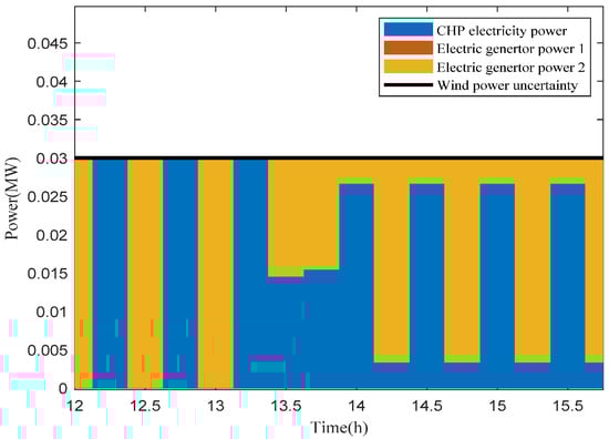
Figure 9.
Reserves of generators and wind power uncertainty in Case I.
4.2. Case II
Compared with Case I, the ramping speed of G2 changes from 0.03 MW/△τ to 0.3 MW/△τ in Case II. The pre-scheduled electricity generation and the balance of supply and demand is depicted in Figure 10. The reserves of generators are shown in Figure 11. It can be seen that only G2 offers 0.03 MW reserve to alleviate the wind power uncertainty. Considering that G2 has sufficient reserve capacity and its reserve cost is cheaper, reserve is completely supplied by G2. From the time 12:00 to 14:00, G1 generation reaches its upper limit and then G2 with the medium operational cost is scheduled to satisfy the remaining electricity load; since no reserve is required from CHP unit and simultaneously the CHP unit generation cost is the most expensive, there is no scheduled CHP unit generation, and the pipelines and buildings are in the heat energy release state, causing the water temperature and indoor temperature to drop. From the time 13:00 to 16:45, G2 generation is kept as 0.03 MW in order to provide sufficient downward reserve; and most of the electricity demand is satisfied by G1 to achieve the economic operation.
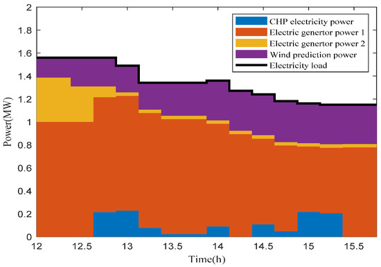
Figure 10.
Pre- scheduled electricity generations and the balance between supply and demand in Case II.
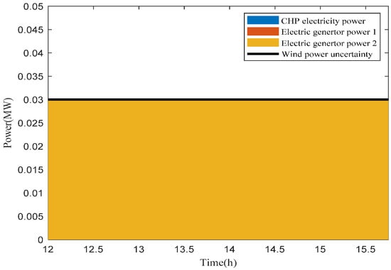
Figure 11.
Reserves of generators and wind power uncertainty in Case II.
Because there is no need for CHP unit to supply reserve to accommodate the fluctuation of wind power, as shown in Figure 12, the indoor temperatures of buildings and the water temperatures at the outlets of heat loads all reach at their lower bounds, induced by the optimization objective of economic operation. The comparison of reserve and operational cost between Cases I and II are listed in Table 3. Owing to the enhanced ramping speed of G2, more G2 electricity generations and reserves in Case II decrease the corresponding cost, compared with Case I. Moreover, Due to the less CHP unit generation, the heat network always stays in the state of releasing energy. As a result, the water temperatures in the pipelines and indoor temperature in buildings show the downward trend, which can be seen in Figure 13 and Figure 14.
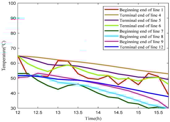
Figure 12.
Pre-scheduled water temperature of heat network in Case II.
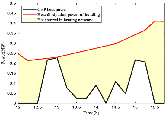
Figure 13.
Pre-scheduled heat energy charging and discharging in Case II.
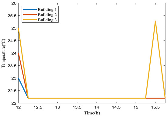
Figure 14.
Pre-scheduled building indoor temperature in Case II.
4.3. Case III
The pre-scheduled electricity generations are drawn in Figure 15. Comparison of electricity generations during different time periods are given in Table 4. From 12:00–14:00, more CHP unit generation is scheduled owing to the lower price; while from 14:15–16:00, G1 generates more electricity. The scheduling results represent the operational economics.
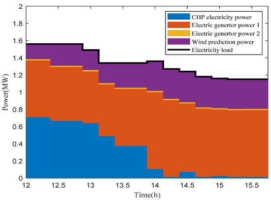
Figure 15.
Pre-scheduled electricity generations and the balance between supply and demand in Case III.
Table 4.
Comparison of electricity generations under time-of-use price.
Pre-scheduled water temperature of heat network is displayed in Figure 16. It can be seen that, the outlet temperature of the heat station drops first and then rises, consistent with the load inlet temperature. However, the turning point for outlet of the heat station appears at 12:15–13:15 while the load outlet at 13:15–14:30. This shows that it takes some time for hot water flowing from heat station to load. Heat production and consumption are not balanced in real time. It is very necessary to conduct transient analysis on the heat network. The water temperatures in Figure 16 are higher than those in Figure 6 and Figure 12, caused by the cheaper cost coefficient of CHP unit generation during 12:00–14:00.
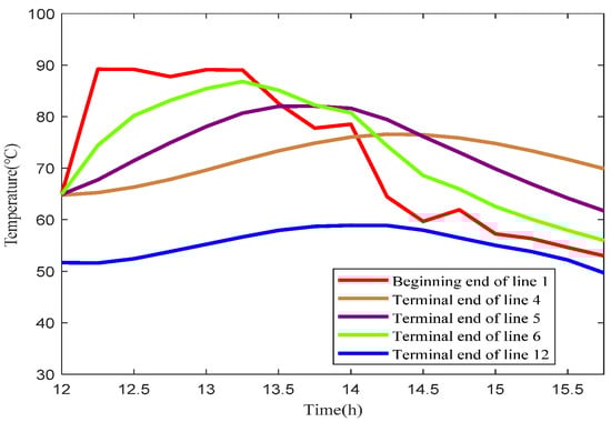
Figure 16.
Pre-scheduled water temperature of heat network in Case III.
4.4. Case IV
In Case IV, both time-of-use price and the thermal storage capacity of heat network and buildings are not concerned. Assuming that the temperature of the building is kept at 23 °C constantly, and the heat dissipation from indoor to outdoor is regarded as heat load. Heat network is simplified to be three heat load nodes. The heat supply and demand are balanced instantaneously for no heat reserve is supplied. The wind power is absorbed as much as possible under the condition of satisfying the operational constraints. The absorbed and abandoned wind power is depicted in Figure 17.
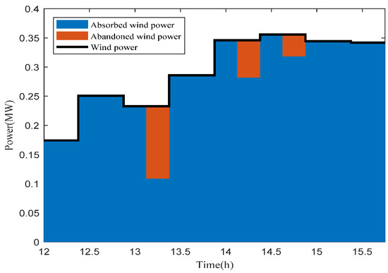
Figure 17.
Absorbed and abandoned wind power in Case Ⅳ.
The electricity generators G1 and G2 are limited to their ramping speed, and the CHP unit working in constant heat-to-electricity ratio mode is subjected to real-time heat balance. It is difficult for all of them to respond to the wind power fluctuation, inevitably leading to wind abandonment. Wind power abandonment occurs at three instants and the maximum abandonment appears at 13:15, with about 53.18% wind power abandoned; on the contrary, the wind absorption is 100% if the thermal storage capacity is considered, as shown in Cases I, II and III. What is more, it will lead to infeasibility under wind power uncertainty for there is no heat reserve in Case IV.
4.5. Discussions on Robustness and Economics
To verify the robustness of the proposed method, 10,000 scenarios are generated by Monte Carlo sampling within the wind prediction boundaries to simulate the real wind power uncertainty. The price coefficient is chosen the same as Cases I, II and IV, listed in Table 2. According to (3), the appropriate value = 6 is chosen, whose corresponding pre-scheduled electric power generation and reserve results have been given in Figure 5 and Figure 9, and heat energy results have been depicted in Figure 7. With the pre-scheduled results of generations and reserves, the re-dispatching problem could derive the feasible solutions of re-dispatched generations under all the 10,000 uncertain wind power realizations. The robustness of the proposed pre-scheduling and re-dispatching coordination approach is validated. As shown in Table 5, if the smaller value is chosen, the feasibility of re-dispatching problem under any uncertain wind power realization might not be guaranteed, with the unfeasibility proportion about 5.55% among the 10,000 wind power realizations, although the total cost could be decreased. On the contrary, with the larger value , the derived total cost in pre-scheduling optimization increases and even worse the computing burden is significantly exacerbated, consuming the computational time several hundred times as much as = 6 due to the less feasibility domain.
Table 5.
Comparisons in robustness, economics and computational costs.
In order to evaluate the superiority of the proposed approach, the interval optimization [16,17,18] and scenario-based optimization methods [19,20,21] are employed for comparison. In the interval optimization method, the robust feasibility constraints are added iteratively as described in Section 2.3 to solve the pre-scheduling problem. The best and worst optimal solutions of interval optimization considering robust feasibility constraints are given in Table 5. It is shown that the robustness can be guaranteed, but their total costs are respectively 2.17% and 8.02% higher compared with the robust economic scheduling. In the scenario-based optimization method, the wind power scenarios are sampled by the Monte Carlo simulations, and reduced by the backward reduction method. In Table 5, N1 and N2 mean the scenario number before and after the scenario reduction. For the reduced scenarios, the feasible iterations are carried out. The total costs of scenario-based optimization methods are lower, but the safe operation of the system cannot be guaranteed when facing the uncertain wind power realization. Under the pre-scheduling results derived by 1000 scenarios-based optimization, the infeasibility proportion of re-dispatching is still about 65.57%. Both of the methods, i.e., the interval optimization and the scenario-based optimization, will face the combinatorial explosion problem as time horizon increases, indicated by the iterations in Table 5. Although the scene reduction can decrease the number of scenarios, its calculation time also cannot be ignored.
Consequently, the robust economic scheduling approach can ensure the feasibility of re-dispatching problem under any uncertain wind power realization while ensuring the economics of scheduling solution. Furthermore, the combination explosion problem can be solved.
5. Conclusions
A two-stage robust economic scheduling is proposed for electricity-heat IES to cope with the wind power uncertainty. In pre-scheduling, while ensuring the economics of scheduling results, the sufficient regulation margin subjected to the operational bounds is reserved for the possible uncertain wind power realization by considering the robust feasibility constraint of re-dispatching. With the pre-scheduling solution, for electric system the appropriate generation reserve is kept to achieve the flexibility, and for heat system, the inherent thermal energy storage of buildings and heat network is utilized to compensate for the fluctuations of heat power generation from CHP unit caused by wind power uncertainty. The thermal storage capability is characterized by modeling the dynamics of building and heat network. The simulation indicates that the proposed approach could enhance the flexibility of heat and electricity coupled system in wind power accommodation. Furthermore, the appropriate choosing of uncertain budget could achieve the robustness and economics of scheduling results at the lower computational cost. The optimization objective of the total cost derived by the proposed approach is lower than the traditional interval optimization. The proposed approach is more robust compared with the traditional scenario-based optimization method. Gradient explosion problem existing in the two traditional methods could be avoided by the proposed approach. The superiority of the proposed approach can be demonstrated.
In cold seasons, with large heat demand and abundant wind power, the fixed heat-power ratio of CHP unit could cause problems in wind accommodation and more importantly, the safe operation of the system, especially in Northeast China. The proposed method can effectively enhance wind power accommodation and achieve robustness and economics of scheduling. In the future research, the uncertainties of electricity demand and heat network parameters will be further considered.
Author Contributions
Conceptualization, R.L. and Z.B.; methodology, R.L., Z.B.; software, R.L.; validation, R.L., Z.B.; formal analysis, R.L., Z.B., J.Z., L.L., M.Y.; investigation, R.L., Z.B., J.Z., L.L., M.Y.; resources, R.L., Z.B., J.Z., L.L., M.Y.; data curation, R.L.; writing—original draft preparation, R.L.; writing—review and editing, R.L., Z.B.; visualization, R.L., Z.B.; supervision, Z.B.; project administration, Z.B., J.Z., L.L., M.Y.; funding acquisition, Z.B., J.Z., L.L., M.Y. All authors have read and agreed to the published version of the manuscript.
Funding
This work was funded by the Key Research and Development Program of Zhejiang Province, Grant Number 2021C01113, Zhejiang Provincial Natural Science Foundation of China, Grant Number LGG22F030008, and National Natural Science Foundation of China, Grant Number 51777182.
Institutional Review Board Statement
Not applicable.
Informed Consent Statement
Not applicable.
Conflicts of Interest
The authors declare no conflict of interest.
Nomenclature
| Indices and Sets | |
| O | the set of branches or pipelines directly connected with a bus or node |
| τ | time index for heat network |
| d | index of electric network slack node |
| g | node index of heat load |
| i | index of heat network node |
| j, l | index of heat pipeline |
| k | index of pipeline segment |
| m, n | indices of electric network buses |
| r | node index of heat exchange station |
| time index for electricity network | |
| Superscript and Subscript | |
| CHP | CHP (combined heat and power) unit |
| b | insulation layer |
| dis | heat dissipation of building |
| down | downward ramping |
| e1 | electric generator with large system inertia |
| e2 | electric generator with small system inertia |
| ex | heat exchange station |
| in | inner layer of pipeline or indoors |
| inject | power injection |
| load | electric or heat load |
| out | outer layer of pipeline or outdoors |
| p | pre-scheduled value or wind power predicted value |
| r | re-dispatched value or real wind power value |
| s | soil layer |
| up | upward ramping |
| w | water flow layer |
| wind | wind power |
| Input Parameters | |
| A | heat transfer coefficient of building fence [W/(m2·°C)] |
| D | diameter of pipeline [m] |
| E | total number of buildings |
| F | equivalent specific heat capacity of building [J/(kg·°C)] |
| G | equivalent mass of building [kg] |
| L | length of the pipeline [m] |
| M | mass flow rate in pipeline [kg/s] |
| N/U | time horizon length of pre-scheduling/re-dispatching |
| R | thermal resistance [(m·K)/W] |
| S | area of the fence [m2] |
| Z | buried depth of pipeline [m] |
| λ | thermal conductivity [W/(m·K)] |
| ρ | density [kg/m3] |
| η | energy utilization coefficient |
| a | price coefficient of operation [$/(MW·min)] |
| b | reactance [pu] |
| c | specific heat capacity [J/(kg·K)] |
| h | convection heat transfer rate [W/(m2·K)] |
| k | heat-to-electricity ratio of CHP unit |
| q | price coefficient of reserve [$/(MW·min)] |
| △t | timescale of heat network [min] |
| △τ | timescale of electricity network [min] |
| △x | segment length of heat pipeline [m] |
| Decision Variables | |
| , | heat power generation of CHP unit at time in pre-scheduling/re-dispatching [W] |
| , | heat power dissipation of building at time in pre-scheduling/re-dispatching [W] |
| , | heat power absorbed by building at time in pre-scheduling/re-dispatching [W] |
| , | electric power generation of CHP unit at time in pre-scheduling/ in re-dispatching [W] |
| , | electric power generation of electric Generator 1 at time in pre-scheduling/re-dispatching [W] |
| , | electric power generation of electric Generator 2 at time in pre-scheduling/ in re-dispatching [W] |
| ,, | reserve of electric Generator 1/electric Generator 1/CHP unit at time / [W] |
| , | temperature of insulation layer/water flow at k-th segment of pipeline l at time in pre-scheduling [K] |
| , | temperature of insulation layer/water flow at k-th segment of pipeline l at time in re-dispatching [K] |
| , | indoor temperature of building at time in pre-scheduling/re-dispatching [°C] |
| , | voltage phase angle at bus m at time in pre-scheduling/ in re-dispatching [rad] |
Appendix A
Table A1.
Simulation parameters.
Table A1.
Simulation parameters.
| Parameters | Value | Parameters | Value | Parameters | Value |
| /min | 30 | 1 | AhSh/(MW·°C)−1 | 7.5 × 10⁻³ | |
| /min | 15 | 1 | FhGh/(MJ·°C)−1 | 7.5 × 10⁻² | |
| /m | 50 | /MW | 3 | /MW | 0 |
| 16 | /MW | 0 | /MW | 1 | |
| 3 | λb/W·(m·K)−1 | 0.033 | /MW | 0 | |
| 1 | Z/m | 1 | /MW | 1 | |
| /°C | 90 | λs/W·(m·K) −1 | 0.31 | /MW | 0 |
| /°C | 30 | cb/J·(kg·°C) −1 | 1380 | /MW | 1 |
| cw/J·(kg·°C)−1 | 4200 | ρb/(kg·m−3) | 1000 | θmax/° | 5 |
| ρw/(kg·m−3) | 1000 | αs/W (m2·K)−1 | 14 | θmin/° | −5 |
| Din/m | 0.4 | M4, τ/(kg·s)−1 | 1.5 | /MW | 0.3 |
| Dout/m | 0.6 | M5, τ/(kg·s)−1 | 1.5 | /MW | 0.3 |
| hwp/W·(m2·K)−1 | 7000 | M6, τ/(kg·s)−1 | 1.5 | /MW | 0.3 |
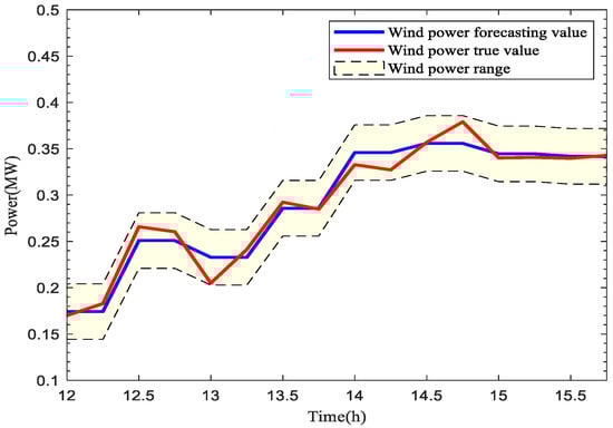
Figure A1.
Wind power forecasting and true value under ±0.03 uncertainty.
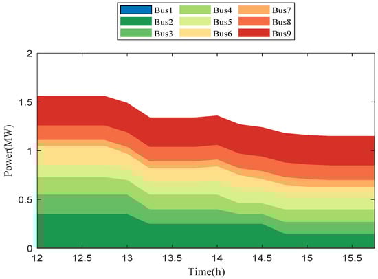
Figure A2.
Electric load of each bus in power system.
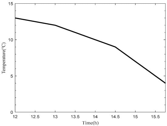
Figure A3.
Outside temperature of buildings.
References
- Tan, L.; Han, J.; Zhang, H. Ultra-Short-Term Wind Power Prediction by Salp Swarm Algorithm-Based Optimizing Extreme Learning Machine. IEEE Access 2020, 8, 44470–44484. [Google Scholar] [CrossRef]
- Nuytten, T.; Claessens, B.; Paredis, K.; Van Bael, J.; Six, D. Flexibility of a Combined Heat and Power System with Thermal Energy Storage for District Heating. Appl. Energy 2013, 104, 583–591. [Google Scholar] [CrossRef]
- Li, Y.; Wang, C.; Li, G.; Wang, J.; Zhao, D.; Chen, C. Improving Operational Flexibility of Integrated Energy System with Uncertain Renewable Generations Considering Thermal Inertia of Buildings. Energy Convers. Manag. 2020, 207, 112526. [Google Scholar] [CrossRef] [Green Version]
- Wang, L.; Li, Q.; Sun, M.; Wang, G. Robust Optimisation Scheduling of CCHP Systems with Multi-Energy Based on Minimax Regret Criterion. IET Gener. Transm. Distrib. 2016, 10, 2194–2201. [Google Scholar] [CrossRef]
- Zhang, C.; Dong, Z.; Xu, Y.; Chen, Y. A Two-Stage Robust Operation Approach for Combined Cooling, Heat and Power Systems. In Proceedings of the 2017 IEEE Conference on Energy Internet and Energy System Integration (EI2), Beijing, China, 26–28 November 2017; pp. 1–6. [Google Scholar]
- Li, Y.; Zou, Y.; Tan, Y.; Cao, Y.; Liu, X.; Shahidehpour, M.; Tian, S.; Bu, F. Optimal Stochastic Operation of Integrated Low-Carbon Electric Power, Natural Gas, and Heat Delivery System. IEEE Trans. Sustain. Energy 2018, 9, 273–283. [Google Scholar] [CrossRef]
- Li, Z.; Wu, W.; Shahidehpour, M.; Wang, J.; Zhang, B. Combined Heat and Power Dispatch Considering Pipeline Energy Storage of District Heating Network. IEEE Trans. Sustain. Energy 2016, 7, 12–22. [Google Scholar] [CrossRef]
- Li, Z.; Wu, W.; Wang, J.; Zhang, B.; Zheng, T. Transmission-Constrained Unit Commitment Considering Combined Electricity and District Heating Networks. IEEE Trans. Sustain. Energy 2016, 7, 480–492. [Google Scholar] [CrossRef]
- Dai, Y.; Chen, L.; Min, Y.; Chen, Q.; Hao, J.; Hu, K.; Xu, F. Dispatch Model for CHP With Pipeline and Building Thermal Energy Storage Considering Heat Transfer Process. IEEE Trans. Sustain. Energy 2019, 10, 192–203. [Google Scholar] [CrossRef]
- Pan, Z.; Guo, Q.; Sun, H. Feasible Region Method Based Integrated Heat and Electricity Dispatch Considering Building Thermal Inertia. Appl. Energy 2017, 192, 395–407. [Google Scholar] [CrossRef]
- Chen, Y.; Xu, Y.; Li, Z.; Feng, X. Optimally Coordinated Dispatch of Combined-Heat-and-Electrical Network with Demand Response. IET Gener. Transm. Distrib. 2019, 13, 2216–2225. [Google Scholar] [CrossRef]
- Good, N.; Karangelos, E.; Navarro-Espinosa, A.; Mancarella, P. Optimization Under Uncertainty of Thermal Storage-Based Flexible Demand Response With Quantification of Residential Users’ Discomfort. IEEE Trans. Smart Grid 2015, 6, 2333–2342. [Google Scholar] [CrossRef]
- Wei, W.; Liu, F.; Mei, S. Robust and Economical Scheduling Methodology for Power Systems Part One Theoretical Foundations. Autom. Electr. Power Syst. 2013, 37, 37–43. (In Chinese) [Google Scholar] [CrossRef]
- Gao, S.; Jurasz, J.; Li, H.; Corsetti, E.; Yan, J. Potential Benefits from Participating in Day-Ahead and Regulation Markets for CHPs. Appl. Energy 2022, 306, 117974. [Google Scholar] [CrossRef]
- Gagge, A.P.; Fobelets, A.P.; Berglund, L.G. A Standard Predictive Index of Human Response to the Thermal Environment. ASHRAE Trans. 1986, 92, 2B. [Google Scholar]
- Liu, Y.; Jiang, C.; Shen, J.; Hu, J. Coordination of Hydro Units with Wind Power Generation Using Interval Optimization. IEEE Trans. Sustain. Energy 2015, 6, 443–453. [Google Scholar] [CrossRef]
- Huang, H.; Li, F.; Mishra, Y. Modeling Dynamic Demand Response Using Monte Carlo Simulation and Interval Mathematics for Boundary Estimation. IEEE Trans. Smart Grid 2015, 6, 2704–2713. [Google Scholar] [CrossRef]
- Bai, L.; Li, F.; Cui, H.; Jiang, T.; Sun, H.; Zhu, J. Interval Optimization Based Operating Strategy for Gas-Electricity Integrated Energy Systems Considering Demand Response and Wind Uncertainty. Appl. Energy 2016, 167, 270–279. [Google Scholar] [CrossRef] [Green Version]
- Heitsch, H.; Römisch, W. Scenario Reduction Algorithms in Stochastic Programming. Comput. Optim. Appl. 2003, 24, 187–206. [Google Scholar] [CrossRef]
- Razali, N.M.M.; Hashim, A.H. Backward Reduction Application for Minimizing Wind Power Scenarios in Stochastic Programming. In Proceedings of the 2010 4th International Power Engineering and Optimization Conference (PEOCO), Shah Alam, Malaysia, 23–24 June 2010; pp. 430–434. [Google Scholar]
- Shu, Z.; Jirutitijaroen, P. Latin Hypercube Sampling Techniques for Power Systems Reliability Analysis with Renewable Energy Sources. IEEE Trans. Power Syst. 2011, 26, 2066–2073. [Google Scholar]
Publisher’s Note: MDPI stays neutral with regard to jurisdictional claims in published maps and institutional affiliations. |
© 2021 by the authors. Licensee MDPI, Basel, Switzerland. This article is an open access article distributed under the terms and conditions of the Creative Commons Attribution (CC BY) license (https://creativecommons.org/licenses/by/4.0/).