A Distributed Hierarchical Control Framework for Economic Dispatch and Frequency Regulation of Autonomous AC Microgrids

Abstract

Motivated by the single point of failure and other drawbacks of the conventional centralized hierarchical control strategy, in this paper, a fully distributed hierarchical control framework is formulated for autonomous AC microgrids. The proposed control strategy operates with a distinct three-layer structure, where: a conventional droop control is adopted at the primary layer; a distributed leaderless consensus-based control is adopted at the secondary layer for active power and, hence, frequency regulation of distributed generating units (DGUs); and the tertiary layer is also based on the distributed leaderless consensus-based control for the optimal power dispatch. Under the proposed strategy, the three constituent control layers work in a coordinated manner. Not only is the load dispatched economically with a negligible power mismatch, but also the frequencies of all the DGUs are regulated to the reference value. However, the frequency regulation is achieved without requiring any central leader agent that has been reported in the contemporary distributed control articles. As compared to the conventional centralized hierarchical control, the proposed strategy only needs local inter-agent interaction with a sparse communication network; thus, it is fully distributed. The formulated strategy is tested under load perturbations, on an autonomous AC microgrid testbed comprising both low-inertia-type (inverter-interfaced) and high-inertia (rotating)-type DGUs with heterogeneous dynamics, and found to successfully meet its targets. Furthermore, it can offer the plug-and-play operation for the DGUs. Theoretical analysis and substantial simulation results, performed in the MATLAB/Simulink environment, are provided to validate the feasibility of the proposed control framework.

1. Introduction

For the past few decades, there has been a growing pressure on the electric power industry regarding the restructuring of the conventional power system due to environmental, economic, and technological concerns. This has led to the concept of microgrids. The preliminary idea of microgrid was presented by R. H. Lasseter in the early 2000s [1,2,3]. He defined a microgrid to be a small-scale, low-voltage electric power distribution system comprising a cluster of distributed generating units (DGUs) or micro-generation sources, energy-storage systems (ESSs), various loads and interconnecting power lines. A microgrid is equipped with its own control and energy-management system [4] enabling it to operate either independently (i.e., autonomously) or in grid-connected mode. It is the fundamental building block of the future smart grid [5], and has gained significant popularity recently due to its several desired attributes, such as enhanced stability, efficiency, reliability and scalability etc. [6]. The common distributed generation technologies include both renewable and non-renewable-type energy sources, such as photovoltaic modules, wind turbines, hydropower, fuel cells, gasoline or diesel-fueled backup generators etc. [7].

A microgrid needs to be provided with a suitable control system for stable, reliable and economic operation. This control system is a decision-making set of software and/or hardware [8,9], and typically possesses a hierarchical structure with three different control layers, namely: primary, secondary and tertiary. Each control layer is designed to meet certain objectives and their execution rates are different. The main goals of the microgrid control system are as follows [8,9,10]: (i) frequency and voltage regulation to their desired reference values in each operating mode, (ii) maintaining a power supply–power demand balance, (iii) ensuring economic operation and demand side management, and (iv) seamless transition between different operating modes. The grid-tied operation is the normal mode of operation for a microgrid, in which the microgrid control is simple, because the larger upstream main grid dominates the dynamics of the microgrid. In this mode, the main grid commands the frequency and voltage, because of having large synchronous generators with large rotating inertia. As a result, the microgrid must synchronize with the main grid in the grid-tied mode. However, due to some disturbance (whether pre-planned or unplanned) the microgrid can also switch to the autonomous mode. In the autonomous mode, the microgrid control is crucial for frequency and voltage stability, reliable power delivery and proper load sharing [11,12,13].

The primary control layer is normally implemented as a local droop controller at each DGU, and subsequent to autonomous mode, it ensures the frequency and voltage stability of the microgrid by restricting their values to pre-defined ranges [13]. However, it might not completely restore the microgrid frequency and voltage due to their dependency on the load. Therefore, the microgrid frequency and voltage deviations, caused by the primary controller, are compensated and restored to the desired values by an additional secondary control layer [13,14,15]. The secondary controller executes for a longer time frame and with a slower dynamic response (i.e., slower execution rate) than the primary controller. This time-scale difference justifies the independent operation and individual design of the two controllers [11,13,15,16,17,18]. The tertiary controller is responsible for economic operation and power flow optimization of the microgrid, and executes for a longer time frame with a slower dynamic response than both the primary and secondary controllers [10,11,19,20,21]. Generally, the economic operation of the microgrid is guaranteed, if all the DGUs operate at the same marginal costs (or incremental costs i.e., total cost per unit power generated) [10].

The secondary controller is implemented as a (i) conventional centralized controller (requiring complex communication network and having heavy computation burden, higher cost, lower reliability and prone to single point of failure issue), (ii) decentralized controller (having higher cost and higher reliability), and (iii) distributed controller (having lower cost and higher reliability) [19,22]. Conventionally, the tertiary controller also exploits a centralized structure [11], and is prone to the same problems as mentioned regarding the centralized secondary controller.

The distributed control of microgrids is inspired by the theory of multi-agent systems (MASs), according to which the microgrid itself is regarded as a MAS and its DGUs (i.e., energy generation nodes) as agents. In this strategy, the coordination among various DGUs is achieved via exchange of information (i.e., communication) according to some restricted communication protocols. The DGUs in a microgrid are physically interconnected via an electric power network. Above this physical layer, there is a cyber layer comprising a sparse (or mild) communication network among DGUs, which is more reliable and cheaper. This communication network can be modeled by a communication graph. Each DGU is permitted to communicate with its neighboring DGUs only. Furthermore, the control protocols are distributed among DGUs, thus overcoming the single point of failure and improving the reliability [11,13,23,24].

Recently, a distributed hierarchical control framework has been reported for a droop-control AC microgrid in [25], which was applicable during autonomous mode, grid-connected mode and any transition mode between the stated two modes. The proposed strategy was operating with a three-layer control structure: at the primary layer, the conventional droop control was adopted; at the secondary level, a distributed leader–follower consensus control was adopted; and at the tertiary level, a PI-based mode-supervisory control strategy was adopted. Since, for frequency and voltage restoration it relied on the leader–follower consensus, hence, the leader agent (i.e., a central or specialized node) was required to coordinate the functions of all the follower agents. Thus, being distributed, it again poses a kind of single point of failure problem in case of leader outage. In [26], the authors have proposed a droop-free hierarchical control framework for inverter-interfaced AC microgrids, capable of operating in both autonomous and grid-connected modes, and where the control objectives were power-sharing, frequency and voltage regulation, and the optimal power dispatch. However, apart from local controllers at each DGU, it also required a microgrid central controller (MGCC) with a central communication system. Thus, it was again susceptible to a single point of failure problem. Similarly, in [27], the authors have proposed a multiple time-scale hierarchical active power balance and frequency stability control framework for medium voltage autonomous AC microgrid, which again needed a MGCC for dynamic stability control. The authors, in [28], have reported a distributed sliding mode control-based frequency regulation and economic dispatch strategy for an autonomous AC microgrid. In the proposed strategy, the tertiary control was merged into the secondary control for speeding up the economic dispatch process. However, the stated article did not report any generation cost parameters and, hence, related (quadratic) cost functions of the DGUs. Instead, the identical incremental cost criterion was established through a consensus algorithm directly using the assumed values of the production costs. Moreover, the power lines were assumed as lossless (i.e., purely inductive). Similarly, the authors in [29], have reported a distributed model predictive (MPC)-based control for frequency regulation and economic operation of an autonomous AC microgrid that could operate with integrated secondary and tertiary control layers. However, the equal production cost criterion was established by straightaway using the assumed values of the incremental costs of DGUs, and then applying a consensus algorithm. In other words, the article did not consider any generation cost coefficients and, hence, the corresponding (quadratic) cost functions of the DGUs. Furthermore, lossless power lines were assumed. The authors of the work reported in [28,29], in the sequel, proposed a distributed MPC-based economic dispatch and frequency regulation strategy for autonomous AC microgrids in [30] that bears the same limitations as described regarding [28,29]. In [31], the authors have proposed a distributed joint operation strategy for hierarchically controlled islanded AC microgrids. However, it relied on the leader agent for frequency and voltage regulation at the secondary control level. Moreover, the distributed secondary frequency and voltage regulation was established using continuous-time consensus algorithms based on single integrator dynamics and having asymptotic convergence. The authors in [32] have reported an event-triggered distributed secondary control framework for frequency regulation and economic dispatch of droop-controlled AC microgrids that demonstrated a comparable performance with the centralized economic dispatch strategy. In [33], the authors have proposed a distributed hierarchical control technique to compensate the voltage variation issue, resulting from the increased integration of photovoltaic system in the distribution networks, by real-time regulation of the reactive power of PV inverters. However, it is noteworthy to state that the contemporary hierarchical control articles [26,27,31,32,33] are focused on the DGUs with homogeneous (or identical) dynamics only. The authors in [34] have reported a multi-agent based distributed power management strategy for voltage regulation and economic power-sharing of diesel generators in DC shipboard power systems. By adjusting the operating speed of each diesel engine, the fuel consumption was minimized up to 10%. However, the stated strategy was focused on DGUs with homogeneous dynamics only. Moreover, the distributed secondary voltage control was based on the continuous-time single integrator dynamics, with asymptotic convergence. In [35], the authors have reported a distributed hierarchical control framework for frequency and voltage regulation in islanded AC microgrids. Moreover, the microgrid operation was optimized by minimizing the overall network power losses using an alternating direction method of multipliers (ADMM) algorithm. However, in the stated strategy both the distributed frequency and voltage regulation were based on (i) the continuous-time single integrator dynamics, with asymptotic convergence, (ii) relying on leader–follower consensus, and (iii) focused on DGUs with homogeneous dynamics only.

Motivation and Major Contributions of the Article

Motivated by the aforementioned drawbacks of the contemporary hierarchical control strategies, the authors have developed an alternative hierarchical control approach suitable for autonomous AC microgrids. The main contributions of this article are listed below:

• A fully distributed hierarchical control framework is formulated for droop-controlled autonomous AC microgrids that guarantees coordinated operation of the three constituent control layers: droop-based primary control, distributed secondary active power and frequency control, and distributed tertiary control for the optimal active power dispatch.
• The suggested scheme operates with a distributed leaderless consensus at both the secondary and tertiary control layers, without needing a leader node to coordinate the functions of the other (i.e., follower) nodes. Consequently, it is not susceptible to single point of failure issue. Since the computational and communication effort is equally distributed among the distributed controllers of DGUs, it is fully distributed in this manner. It is reliable as well as flexible than the contemporary distributed [25,26,27] and conventional centralized control strategies.
• The proposed control framework is tested under plug-and-play event of DGUs and under load perturbations. It is found to dispatch load economically along with regulating frequencies of DGUs to the reference value.
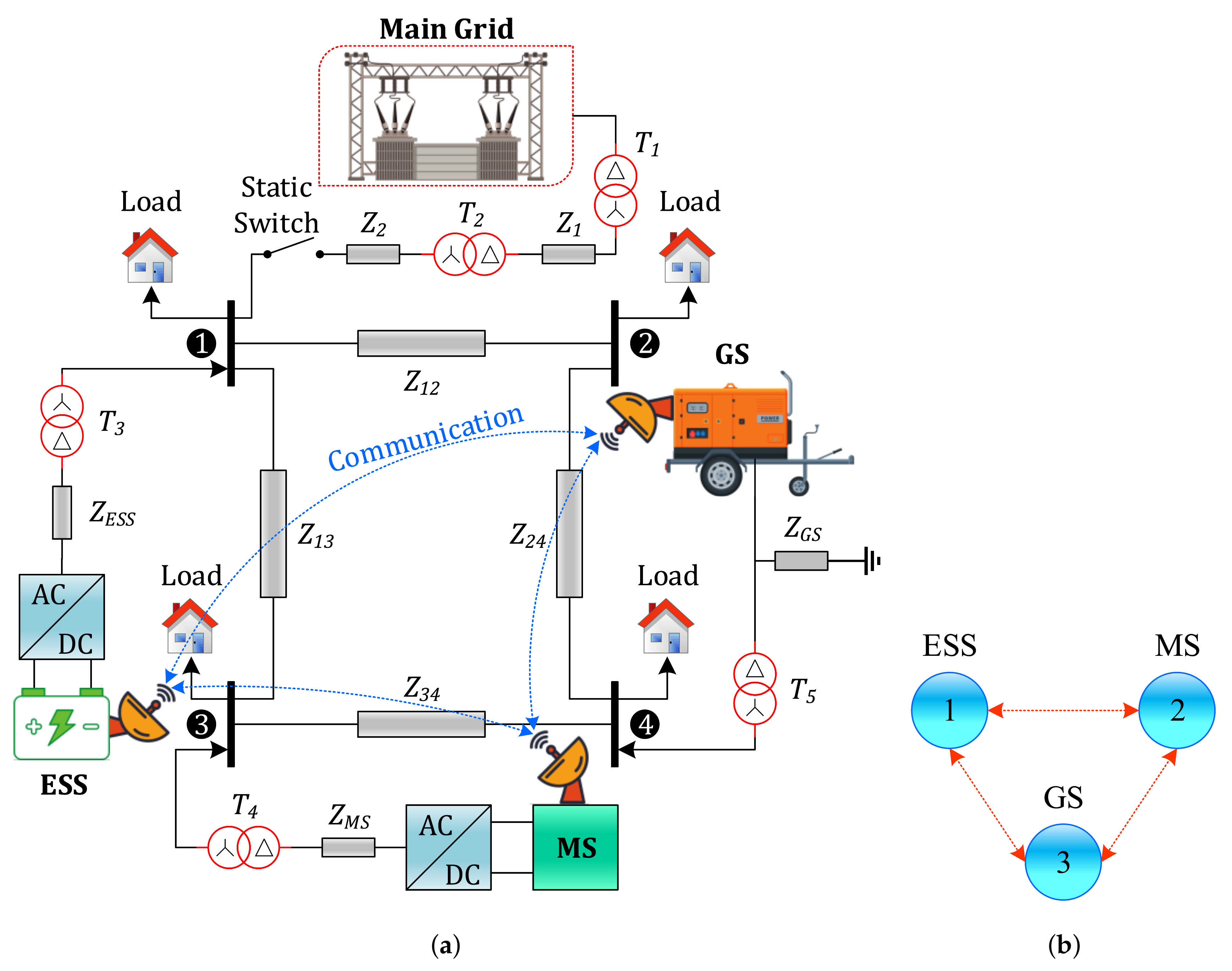
• The microgrid simulation testbed used in this work possesses both low-inertia (converter-interfaced)-type and high-inertia (rotating)-type DGUs. On the other hand, the contemporary articles [26,27,31,32,33] are focused only on the low-inertia-type DGUs. Since, the dynamic response of the high-inertia-type DGUs is slower (due to speed governor) than the low-inertia-type DGUs [36], hence, it becomes a challenging task to formulate a distributed hierarchical control strategy for a microgrid with DGUs that have heterogeneous dynamics, and coordinate their operations successfully. This article addresses this issue.

Remark 1.

This article is written in continuation of the authors’ previous article [37], where the control objectives were: (i) the distributed secondary control of active power of DGUs and, hence, (ii) their frequency regulation to the reference value. Please note that the system had only two control layers, i.e., the primary and secondary control layers.

Now, to further the work presented in [37], in the present article, the authors have also added the tertiary control layer to the previous system, so that the load is economically dispatched with a minimum power mismatch besides the active power control and, hence, frequency regulation of DGUs to the reference value.

The remaining article is organized as follows: Section 2 covers the preliminary communication graph theory. Section 3 describes the microgrid simulation testbed configuration. Section 4 explains the closed-loop implementation strategy of the proposed distributed hierarchical control framework. Section 4.2 verifies the effectiveness of the proposed strategy through various numerical simulation results, performed in the MATLAB/Simulink environment. Lastly, Section 6 concludes this work.

2. Graph Theory

The distributed control of microgrids rely on the theory of multi-agent system (MAS). Using this theory, the communication network between DGUs (i.e., agents) of the microgrid is modeled as a weighted graph, $\mathcal{G}$, as shown in Figure 1b. The vertices of the graph represent the energy nodes or agents, and the edges or arcs represent the communication lines. Now, let $\mathcal{G}(\mathcal{V},\mathcal{E},\mathcal{A})$, be a weighted undirected (i.e., bidirectional) graph, where $\mathcal{V}=\{{\mathcal{V}}_1,{\mathcal{V}}_2,\cdots ,{\mathcal{V}}_N\}$ be the set of vertices, $\mathcal{E}\subset \mathcal{V}\times \mathcal{V}$ be the set of edges and $\mathcal{A}=\left[a_{ij}\right]\in R^{N\times N}$ be the weighted adjacency matrix, where N indicates the number of nodes. An edge $({\mathcal{V}}_i,{\mathcal{V}}_j)\in \mathcal{E}$ indicates an edge from the ith node to the jth node, and implies that the jth node can acquire information from the ith node, and vice versa. There is a communication weight $a_{ij}\ge 0$, associated with each edge $({\mathcal{V}}_j,{\mathcal{V}}_i)\in \mathcal{E}$, such that $a_{ij}>0\forall ({\mathcal{V}}_j,{\mathcal{V}}_i)\in \mathcal{E}$ (i.e., if there is an edge from the jth node to the ith node); otherwise $a_{ij}=0$∀ ($i\ne j,i,j=\{1,2,\cdots ,N\}$). The neighboring node set of the ith node is, ${\mathcal{N}}_i=\{{\mathcal{V}}_j:({\mathcal{V}}_j,{\mathcal{V}}_i)\in \mathcal{E}\}$, and the number of (in-) neighbors of the ith node is $\mid {\mathcal{N}}_i\mid$, and equals its in-degree, $d_i^{in}$. The weighted Laplacian matrix of the graph, $\mathcal{G}$, is given as: $\mathcal{L}={\mathcal{D}}^{in}-\mathcal{A}\in R^{N\times N}$, where ${\mathcal{D}}^{in}$ is the weighted in-degree matrix and defined as: ${\mathcal{D}}^{in}=diag\left\{d_i^{in}\right\}\in R^{N\times N}$ with $d_i^{in}={\sum }_{j\in {\mathcal{N}}_i}{a}_{ij}$ [38].

3. Simulation Testbed Configuration

The performance and effectiveness of the proposed distributed hierarchical control framework is tested and verified on a 3-phase microgrid testbed, as shown in Figure 1a. The stated microgrid testbed comprises three distributed generation units (DGUs) and overall four buses. There are two inverter-interfaced DGUs and one internal combustion engine (ICE)-based DGU i.e., a diesel genset (GS) with a wound-field synchronous generator. The inverter-interfaced DGUs comprise a microsource (MS) and an external energy-storage system (ESS). The three DGUs are connected to the buses in the following order: ESS to bus 1, MS to bus 3 and GS to bus 4. Each DGU is connected to its respective bus using a 3-phase $\Delta$Y-transformer. Bus 1 provides a point of interconnection of the overall microgrid to the main grid using a static transfer switch (STS). Between the DGUs and their respective buses, $Z_{ESS}$ and $Z_{MS}$ indicate the series coupling inductances, and $Z_{GS}$ represents a coupling capacitor. Various loads are connected to the four buses. The line impedances between the main grid and bus 1 (i.e., $Z_1$, $Z_2$) and between the other buses (i.e., $Z_{12}$, $Z_{13}$, $Z_{24}$ and $Z_{34}$) represent $RLC$-branches. The overall microgrid testbed parameters are given in Appendix A, in

Table A2. Microgrid testbed transformers specifications.

TAG	Rating (kVA)	Frequency (Hz)	Primary Winding Specifications			Secondary Winding Specifications
			${\mathit{V}}_{\mathit{ph}-\mathit{ph}}\left(\mathrm{V}\right)$	$\mathit{R}(\Omega )$	${\mathit{X}}_{\mathit{L}}(\Omega )$	${\mathit{V}}_{\mathit{ph}-\mathit{ph}}\left(\mathrm{V}\right)$	$\mathit{R}(\Omega )$	${\mathit{X}}_{\mathit{L}}(\Omega )$
${\mathrm{T}}_1$	2500	60	4160	0.04706	0.1882	480	0.000627	0.0025068
${\mathrm{T}}_2$	75	60	480	0.0169	0.0676	208	0.0003	0.0127
${\mathrm{T}}_3$	45	60	208	0.02688	0.1075	208	0.005047	0.0201
${\mathrm{T}}_4$	45	60	208	0.02688	0.1075	208	0.005047	0.0201
${\mathrm{T}}_5$	45	60	208	0.02688	0.1075	208	0.005047	0.0201

–

Table A4. ICE-based DGU (i.e., diesel genset) specifications.

ICE-Based Diesel Genset Specifications
Quantity	Value	Quantity	Value
$S_{base}$	$12.50$$\mathrm{k}$$\mathrm{VA}$	$X_q$	0.53301
$V_{base}$	208 $\mathrm{V}$	$X_q^{\prime \prime }$	0.051
$f_0$	60 $\mathrm{Hz}$	$X_l$	0.037
$\Delta f$	$0.50$$\mathrm{Hz}$	$T_d^{\prime }$	0.35523
${\omega }_0$	377 $\mathrm{rad}$/$\mathrm{s}$	$T_d^{\prime \prime }$	0.00015
$\Delta \omega$	$\pi$$\mathrm{rad}$/$\mathrm{s}$	$T_q^{\prime \prime }$	0.0067
$P_{max}$	$12.50 \mathrm{k}\mathrm{W} \mathrm{or} 1 \mathrm{pu}$	$R_s$	0.0217 pu
$P_{min}$	0 $\mathrm{k}$$\mathrm{W}$	$H\left(s\right)$	0.1901
$V_{req}$	$208 \mathrm{V} \mathrm{or} 1 \mathrm{pu}$	p	2
$K_{P,p}$	3	$K_{G,p}$	10
$K_{P,i}$	30	$K_{G,i}$	20
$K_{V,p}$	1000	$K_{tf}$	0.625
$K_{V,i}$	10	$K_{ev}$	11.8238
$m_P$	$\pi$	$K_{fv}$	3600
$m_Q$	0.05	${\eta }_{th}$	0.47
${\tau }_V,{\tau }_P,{\tau }_Q$	$0.01$$\mathrm{s}$	${\tau }_d$	$0.022$$\mathrm{s}$
$X_d$	1.204	$K_m$	0.36
$X_d^{\prime }$	0.125	${\tau }_{ex}$	$0.001$$\mathrm{s}$
$X_d^{\prime \prime }$	0.056	...	...

. The communication between DGUs is represented by an undirected graph, $\mathcal{G}$, in Figure 1b.

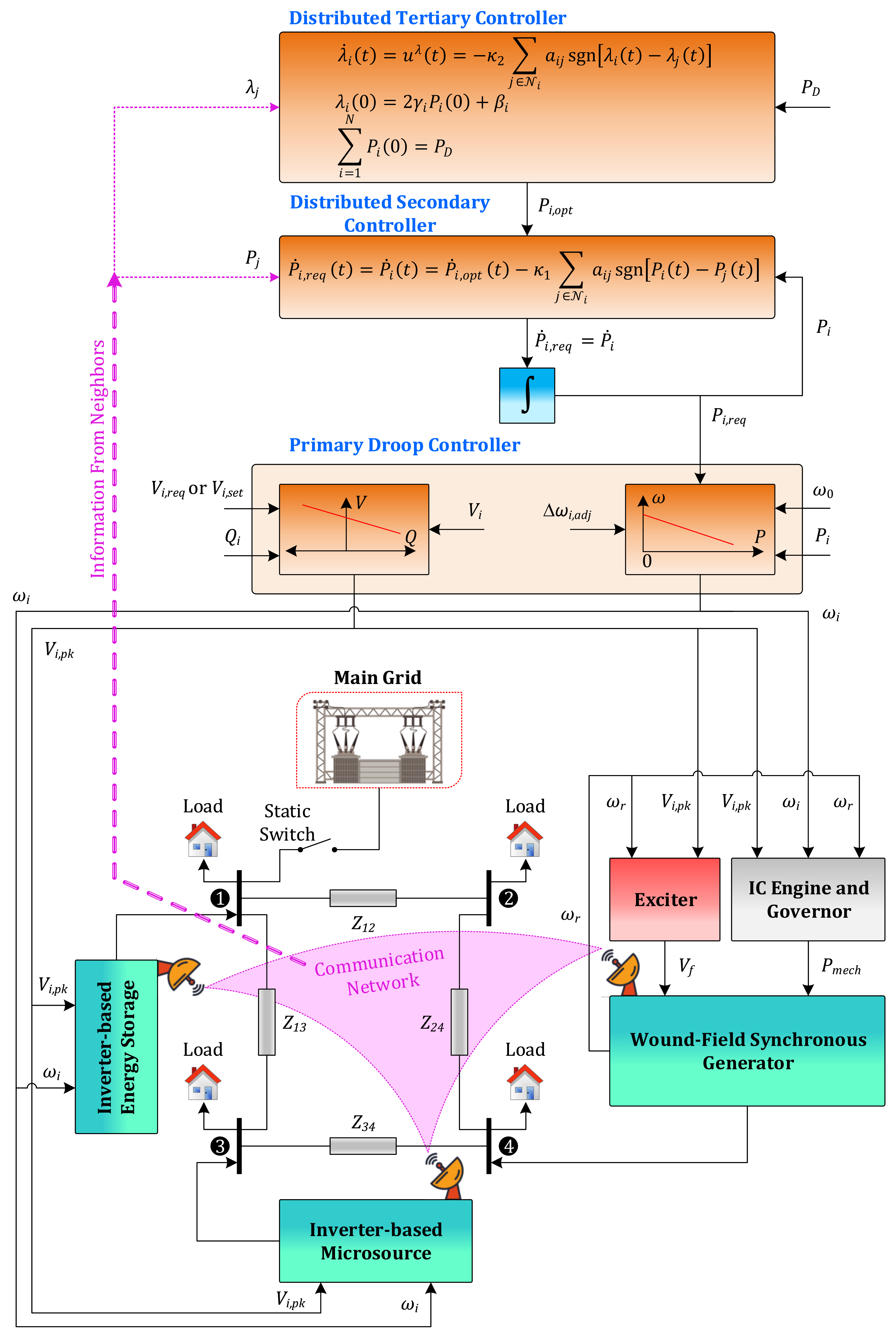
4. Proposed Distributed Hierarchical Control Framework

The closed-loop operation of the overall proposed scheme is illustrated in Figure 2. It comprises three constituent control layers, i.e.: (i) the primary level is provided using the conventional droop control; (ii) the secondary level is implemented using a leaderless consensus-based distributed power and frequency control; and (iii) the tertiary level is also implemented using a leaderless consensus-based distributed economic load dispatch.

The strategy has been designed so that all the three control levels work in a coordinated fashion, and the following intended control objectives are successfully achieved:

• Subsequent to islanding, restore the frequency of each DGU to the microgrid reference frequency, $f_0$, despite load perturbations
• To ensure plug-and-play operation for DGUs
• To dispatch the load economically with a negligible power mismatch

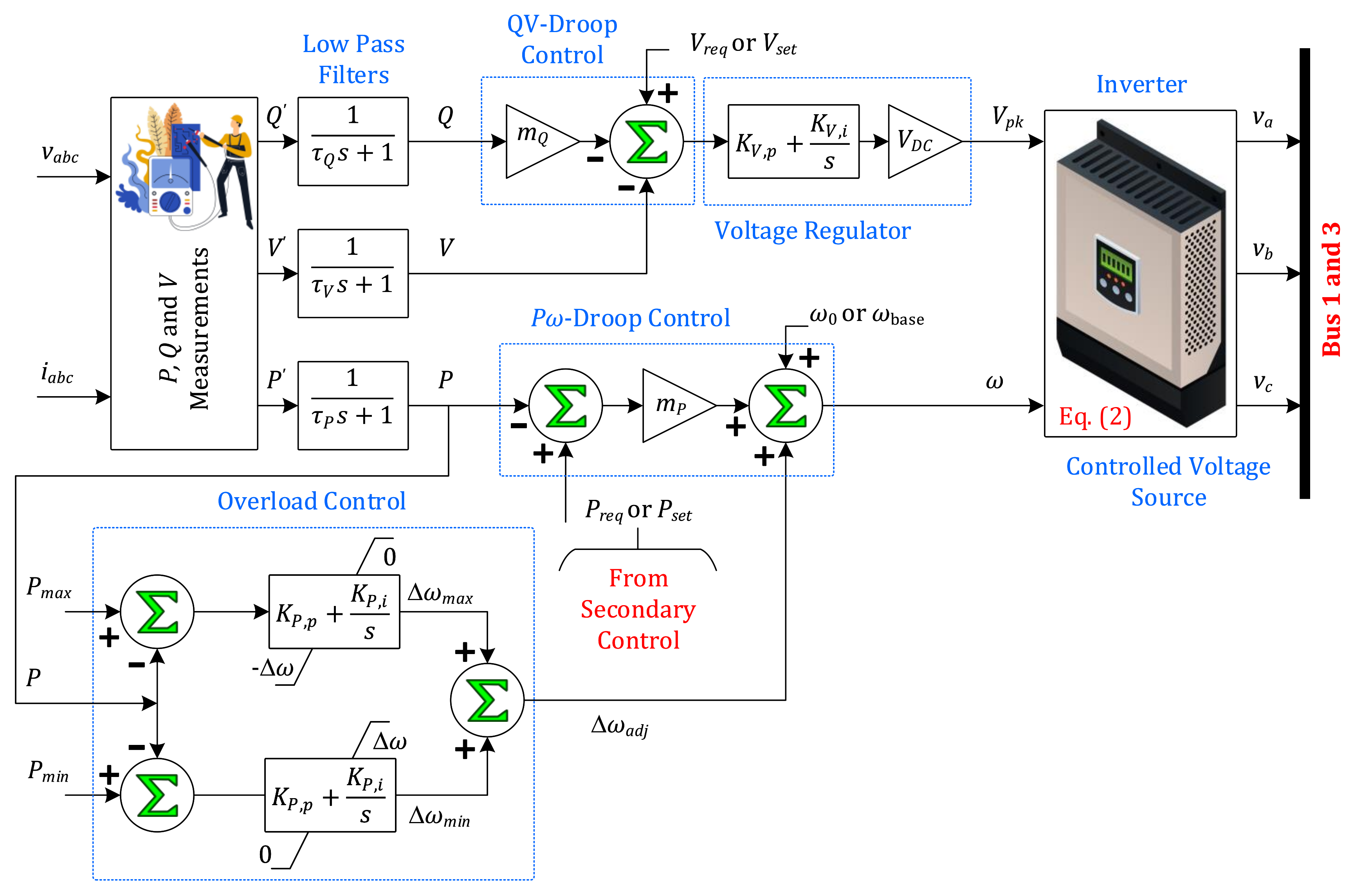
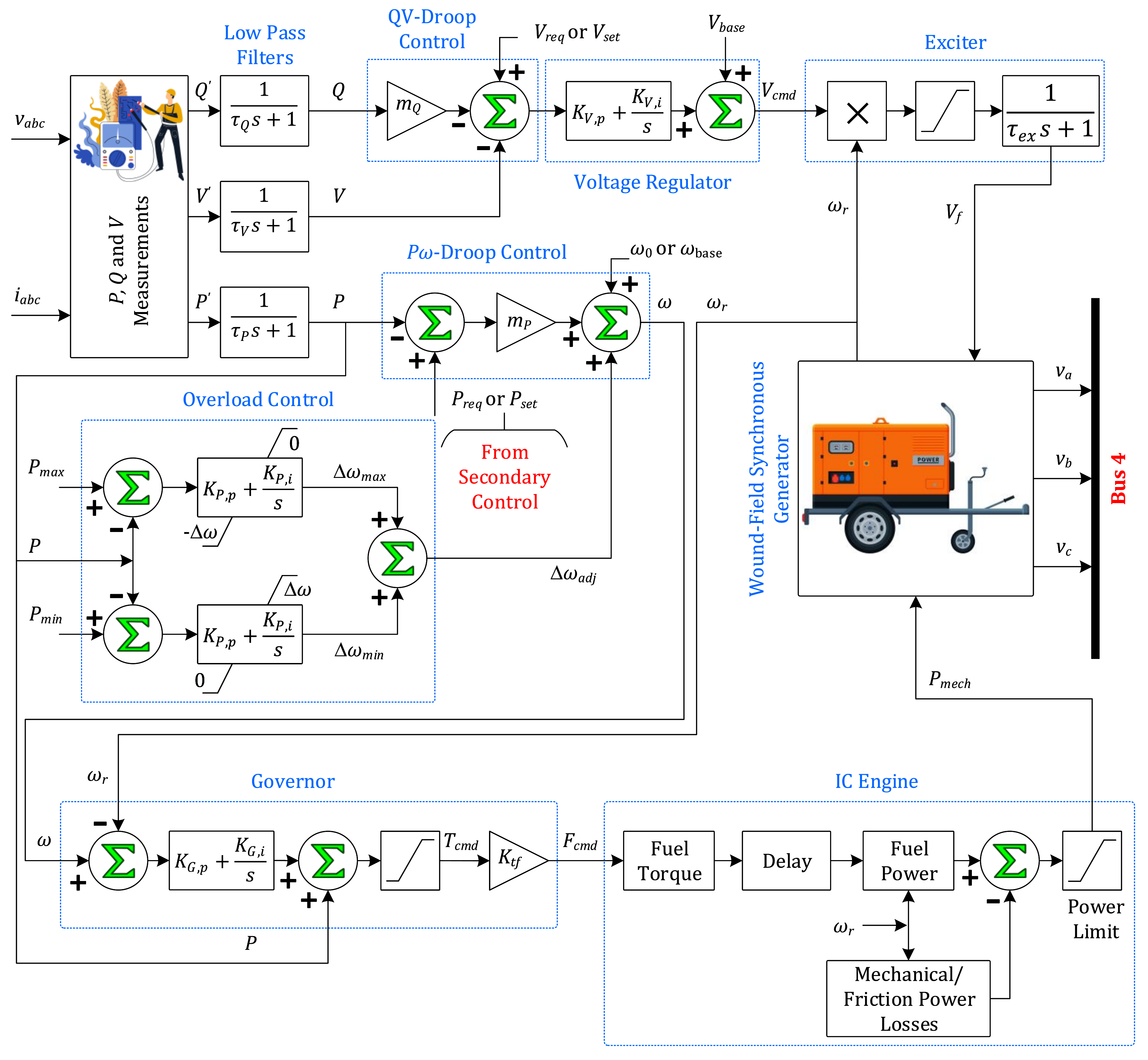
4.1. Primary Control Level

To proportionally share the load power demand between various DGUs and concurrently ensure their frequency and voltage stability, the conventional droop control is frequently employed at the primary control level. For an ith DGU, it can be expressed as follows [39,40]:

$$\left.\begin{array}{ll}\begin{array}{c}P\omega -\mathrm{droop}\mathrm{control}:{\omega }_i\end{array}& ={\omega }_0+\Delta {\omega }_{i,adj}+m_{i,P}\left(P_{i,req}-P_i\right)\\ QV-\mathrm{droop}\mathrm{control}:V_{i,pk}& =V_{i,req}-V_i-m_{i,Q}{Q}_i\end{array}\right\}$$

(1)

where in Equation (1), ${\omega }_i$ is the angular frequency of the ith DGU, ${\omega }_0$ is the reference angular frequency of the microgrid, $\Delta {\omega }_{i,adj}$ denotes the frequency adjustment term provided by the overload control scheme reported in [41], $m_{i,P}>0$ is the $P\omega$-droop-control gain, $P_{i,req}$ and $P_i$ are, respectively, the real power set-point (i.e., reference signal acquired by the primary (i.e., $P\omega$-droop) controller from the distributed secondary controller) and the locally measured real power output of ith DGU. Moreover, $V_{i,req}$ and $V_i$ are, respectively, the voltage set-point and the locally measured output voltage of ith DGU, $m_{i,Q}>0$ is the $QV$-droop-control gain, and $Q_i$ is the locally measured reactive power output of ith DGU. For inverter-interfaced DGUs (i.e., ESS and MS), $V_{i,pk}$ is the voltage amplitude at the inverter terminals, and for GS, $V_{i,pk}=V_{cmd}$ indicates the voltage command applied to the field-exciter controller for generating field-excitation, $V_f$.

Please note that the inverter-interfaced DGUs are modeled as 3-phase controlled-voltage sources, so that their 3-phase output voltages, as shown in Figure 3, can be expressed as follows [37]:

$$\left.\begin{array}{l}{v}_a=V_{i,pk}sin({\omega }_{i}t+0{}^{\circ })\\ v_b=V_{i,pk}sin({\omega }_{i}t-120){}^{\circ }\\ v_c=V_{i,pk}sin({\omega }_{i}t+120{}^{\circ })\end{array}\right\}$$

(2)

where in Equation (2), $V_{i,pk}=M_D{V}_{DC}$, with $V_{DC}$ and $M_D$, respectively, indicating the inverter DC input voltage and the modulation index.

The primary control strategies for the inverter-interfaced DGUs (i.e., ESS and MS ) and the ICE-based DGU (i.e., diesel GS) are, respectively, illustrated in Figure 3 and Figure 4. The respective simulation parameters are given in Appendix A, in Table A2–Table A4. Please note that the primary control level for inverter-interfaced MS and ESS differs from one another in one respect only. In the case of ESS, the lower limit of real power is negative (i.e., $P_{min}=-2.50 \mathrm{k}\mathrm{W}$), indicating charging/electrical energy storage.

The fuel command, fuel toque, fuel power, and friction power loss expressions (i.e., $F_{cmd}$, $T_F$, $F_p$, and $P_f$, respectively) for GS are given below:

$$\left.\begin{array}{l}\begin{array}{c}{F}_{cmd}=K_{tf}{T}_{cmd}\end{array}\\ T_F={\eta }_{th}{K}_{fv}{K}_{ev}{F}_{cmd}\\ F_p=T_F{\omega }_r\\ P_f=K_m{\omega }_r^2\end{array}\right\}$$

(3)

where in Equation (3), $T_{cmd}$ and ${\omega }_r$ are, respectively, the torque command and speed of rotation of the synchronous generator, and $K_{tf}$, ${\eta }_{th}$, $K_{fv}$, $K_{ev}$ and $K_m>0$ are constants.

4.2. Secondary Control Level

The distributed secondary control ensures real power and, hence, frequency control of each DGU in a finite-time, and counteracts steady-state frequency deviations under load perturbations. As inspired by [42], the stated goal is achieved by proposing the following distributed nonlinear finite-time real power consensus algorithm:

$$\left.\begin{array}{ll}{\dot{\upsilon }}_i\left(t\right)& {\displaystyle =-{\kappa }_1\sum _{j\in {\mathcal{N}}_i}{a}_{ij}sgn\left[P_i\left(t\right)-P_j\left(t\right)\right]}\\ P_i\left(t\right)& ={\upsilon }_i\left(t\right)+r_i\left(t\right)={\upsilon }_i\left(t\right)+P_{i,opt}\left(t\right)\end{array}\right\}$$

(4)

where in Equation (4), $i=\{1,2,\cdots ,N\}$ represents the DGUs index set with $N=3$, ${\kappa }_1>0$ indicates a design parameter, $a_{ij}$ is the entry of the adjacency matrix, A, ${\upsilon }_i\left(t\right)\in {\mathbb{R}}^N$ represents an intermediate state variable, $r_i\left(t\right)=P_{i,opt}\left(t\right)\in {\mathbb{R}}^N$ is the time-varying reference signal (i.e., the optimal power dispatch reference) for an ith DGU acquired by the distributed secondary controller from the distributed tertiary controller.

The main goals of the distributed secondary control algorithm, expressed in Equation (4), are: (i) to force all the agents (i.e., DGUs) of the communication graph, $\mathcal{G}$, to reach a consensus, and (ii) to force an ith agent to track its time-varying optimal power dispatch reference, $P_{i,opt}$, acquired from the distributed tertiary controller and, resultantly, restore the frequencies of the DGUs to the microgrid reference frequency, i.e., for an ith agent one must have,

$$\left.\begin{array}{l}\parallel P_i\left(t\right)-P_{i,opt}\left(t\right)\parallel \to 0\\ \parallel f_i\left(t\right)-f_0\parallel \to 0\end{array}\right\}\mathrm{as}t\to \infty$$

Please note that in Equation (4), (i) $r_i\left(t\right)=P_{i,opt}\left(t\right)$ is differentiable, and (ii) its derivative is bounded. Moreover, $sgn(·)$ indicates a multi-valued signum function expressed as follows:

$$sgn(\beth )=\left\{\begin{array}{cc}\hfill 1\hfill & \hfill \mathrm{if}\beth >0\hfill \\ \hfill 0\hfill & \hfill \mathrm{if}\beth =0\hfill \\ \hfill -1\hfill & \hfill \mathrm{if}\beth <0\hfill \end{array}\right.$$

(5)

Remark 2.

The implementation of Equation (4), which indicates the distributed secondary controller, in this research is quite different from the authors’ previous article [37], where $r_i\left(t\right)=P_{Li,avg}\left(t\right)$ (i.e., the system average real load), so that each DGU dispatched average real load. The previous article covered only the primary and secondary control levels, and there was no tertiary control at all. However, in this article, $r_i\left(t\right)=P_{i,opt}\left(t\right)$ is the optimal power dispatch reference for an ith DGU acquired by the distributed secondary controller from the distributed tertiary controller, so that the load is economically dispatched and, concurrently, the frequencies of DGUs are restored to the reference value. However, this frequency restoration process doesn’t need any dedicated auxiliary frequency control.

For an ith DGU, the intermediate state variable, ${\upsilon }_i\left(t\right)$, is initialized in the following manner:

$$\begin{array}{cc}\hfill {\upsilon }_i\left(0\right)=0\Rightarrow \sum _{i=1}^N{\upsilon }_i\left(0\right)& \hfill =0\hfill \end{array}$$

(6)

Using Equation (4), the following closed-loop distributed secondary control system is deduced by differentiation:

$$\left.\begin{array}{ll}\begin{array}{c}{\dot{P}}_{i,req}\left(t\right)\end{array}& ={\dot{P}}_i\left(t\right)\\ & {\displaystyle ={\dot{\upsilon }}_i\left(t\right)+{\dot{P}}_{i,opt}\left(t\right)={\dot{P}}_{i,opt}\left(t\right)-{\kappa }_1\sum _{j\in {\mathcal{N}}_i}{a}_{ij}sgn\left[P_i\left(t\right)-P_j\left(t\right)\right]}\end{array}\right\}$$

(7)

with the initial conditions ${\sum }_{i=1}^N{P}_i\left(0\right)={\sum }_{i=1}^N{P}_{i,opt}\left(0\right)$.

In Equation (7), $P_{i,req}\left(t\right)$ is the reference signal for the primary (i.e., $P\omega$-droop) controller, generated by the distributed secondary controller. Figure 2 depicts the overall closed-loop operation of the distributed secondary controller.

Convergence Analysis of the Distributed Secondary Controller

The presence of the discontinuous signum function, causes discontinuity in the control algorithm, expressed in Equation (4). Hence, its solution can be perceived in the Filippov sense [43].

Lemma 1.

Let$\mathcal{G}$be a connected communication graph, and$\parallel P_i\left(t\right)-P_j\left(t\right)\parallel =0$, ∀$i,j=\{1,2,\cdots ,N\}$, then$\parallel P_i\left(t\right)-P_{i,opt}\left(t\right)\parallel =0$, for system expressed in Equation (4), ∀$i=\{1,2,\cdots ,N\}$.

Proof. 

Equation (4) implies that:

$$\sum _{i=1}^N{P}_i\left(t\right)=\sum _{i=1}^N{\upsilon }_i\left(t\right)+\sum _{i=1}^N{P}_{i,opt}\left(t\right)$$

(8)

Since, the communication graph, $\mathcal{G}$, depicted in Figure 1b, is undirected, it implies:

$$\sum _{i=1}^N{\dot{\upsilon }}_i\left(t\right)=-{\kappa }_1\sum _{i=1}^N\sum _{j\in {\mathcal{N}}_i}{a}_{ij}sgn\left[P_i\left(t\right)-P_j\left(t\right)\right]=0$$

(9)

As ${\sum }_{i=1}^N{\upsilon }_i\left(0\right)=0$ (see Equation (6)), hence, Equation (9) implies that ${\sum }_{i=1}^N{\upsilon }_i\left(t\right)\equiv 0\forall t\ge 0$. Consequently, one is left with,

$$\sum _{i=1}^N{P}_i\left(t\right)=\sum _{i=1}^N{P}_{i,opt}\left(t\right)\forall t\ge 0$$

(10)

If $\parallel P_i\left(t\right)-P_j\left(t\right)\parallel =0$, ∀$i,j=\{1,2,\cdots ,N\}$, it follows from Equation (10) that $\parallel P_i\left(t\right)-P_{i,opt}\left(t\right)\parallel =0$, ∀$i=\{1,2,\cdots ,N\}$. In other words, the distributed secondary control algorithm, expressed in Equation (4), guarantees that each $P_i\left(t\right)$ approaches its respective $P_{i,opt}\left(t\right)$ in a finite-time. □

4.3. Tertiary Control Level

The tertiary controller prescribes the optimal power dispatch references (i.e., $P_{i,opt}$, where $i=\{1,2,\cdots ,N=3\}$, respectively, refers to ESS, MS and GS) for the distributed secondary controller, expressed in Equation (4) and illustrated in Figure 2. The economic load dispatch (ELD) problem can be solved in a (i) centralized, or (ii) distributed manner.

4.3.1. Centralized Tertiary Controller—Centralized Economic Load Dispatch

Conventionally, the ELD problem is sorted out in a centralized manner. The objective is to minimize the total generation cost, $C_T\left(P_i\right)$, subject to equality and inequality constraints, and is expressed as follows [44,45]:

$$\left.\begin{array}{ll}\begin{array}{c}\end{array}& {\displaystyle \mathrm{Objective}\mathrm{function}:min{C}_T\left(P_i\right)=min\sum _{i=1}^N{C}_i\left(P_i\right)=min\sum _{i=1}^N\left({\alpha }_i+{\beta }_i{P}_i+{\gamma }_i{P}_i^2\right)}\\ & \mathrm{Subject}\mathrm{to}:\left\{\begin{array}{ll}{\displaystyle \sum _{i=1}^N{P}_i=P_D}& (\mathrm{equality}\mathrm{or}\mathrm{power}\mathrm{balance}\mathrm{constraint})\\ P_{i,min}\le P_i\le P_{i,max}& (\mathrm{inequality}\mathrm{or}\mathrm{power}\mathrm{generation}\mathrm{constraint})\end{array}\right.\end{array}\right\}$$

(11)

where $C_i\left(P_i\right)$ represents a quadratic-type generation cost function for the ith DGU, ${\alpha }_i,{\beta }_i,{\gamma }_i>0$ are the generation cost parameters of the ith DGU, $P_i$ is the real power output of the ith DGU, $P_{i,min}$ and $P_{i,max}$ are, respectively, the lower and upper bounds of the power output of the ith DGU, and $P_D$ is the total real power demand.

One of the typical approaches, for solving the ELD problem in a centralized manner, is to apply the Lagrange multiplier method in which the constraints are augmented into the objective function. The Lagrange function, $\mathcal{L}$, for the ELD problem can be formulated as follows:

$$\mathcal{L}\left(P_i,\lambda \right)=C_T\left(P_i\right)+\lambda \left(P_D-\sum _{i=1}^N{P}_i\right)$$

(12)

where $\lambda$ is the Lagrange multiplier corresponding to the power balance constraint given in Equation (11).

Now, the necessary condition for the extreme value of the objective function can be obtained from the first-order optimization conditions, i.e., taking the first derivative of the Lagrange function, $\mathcal{L}$, with respect to each of the independent variables (i.e., $P_i$ and $\lambda$) and then setting the derivatives equal to 0. These conditions are termed as the Karush–Kuhn–Tucker conditions, and are applied as follows:

$$\left.\begin{array}{ll}\begin{array}{c}\mathrm{Condition}1:\end{array}& {\displaystyle \frac{\partial \mathcal{L}}{\partial P_i}=\frac{\partial C_T\left(P_i\right)}{\partial P_i}-\lambda =0⟹\frac{d{C}_i\left(P_i\right)}{d{P}_i}={\lambda }_{opt}=2{\gamma }_i{P}_{i,opt}+{\beta }_i}\\ \mathrm{Condition}2:& {\displaystyle \frac{\partial \mathcal{L}}{\partial \lambda }=P_D-\sum _{i=1}^N{P}_i=0⟹\sum _{i=1}^N{P}_{i,opt}=P_D}\end{array}\right\}$$

(13)

Rearranging condition 1 in Equation (13) for $P_{i,opt}$, yields:

$$P_{i,opt}=\frac{{\lambda }_{opt}-{\beta }_i}{2{\gamma }_i}\ge 0$$

(14)

Substituting $P_{i,opt}$ from Equation (14) into condition 2, given in Equation (13), yields:

$${\lambda }_{opt}=\frac{{\displaystyle P_D+\sum _{i=1}^N\frac{{\beta }_i}{2{\gamma }_i}}}{{\displaystyle \sum _{i=1}^N\frac{1}{2{\gamma }_i}}}$$

(15)

Equation (13) provides the necessary conditions for the existence of the minimum generation cost (i.e., the optimal power dispatch), while considering the equality constraint only, but without considering any inequality constraint (i.e., $P_{i,min}=0$ and $P_{i,max}=\infty$) given in Equation (11), and states that the incremental costs (i.e., $d{C}_i\left(P_i\right)/d{P}_i$) of all the generating units must be equal to the Lagrange multiplier, $\lambda$. This strategy is known as the equal incremental cost criterion.

Now, if the power generation constraint is also recognized (i.e., $P_{i,min}\le P_i\le P_{i,max}$), then the necessary conditions given in Equation (13) for the optimal power dispatch can be interpreted as follows:

$$\left.\begin{array}{l}\begin{array}{c}{\displaystyle \frac{d{C}_i\left(P_i\right)}{d{P}_i}=\frac{{\displaystyle P_D+\sum _{i=1}^N\frac{{\beta }_i}{2{\gamma }_i}}}{{\displaystyle \sum _{i=1}^N\frac{1}{2{\gamma }_i}}}={\lambda }_{opt}\mathrm{for}{P}_{i,min}<P_i<P_{i,max}}\end{array}\\ {\displaystyle \frac{d{C}_i\left(P_i\right)}{d{P}_i}=\frac{{\displaystyle P_D+\sum _{i=1}^N\frac{{\beta }_i}{2{\gamma }_i}}}{{\displaystyle \sum _{i=1}^N\frac{1}{2{\gamma }_i}}}\le {\lambda }_{opt}\mathrm{for}{P}_i=P_{i,max}}\\ {\displaystyle \frac{d{C}_i\left(P_i\right)}{d{P}_i}=\frac{{\displaystyle P_D+\sum _{i=1}^N\frac{{\beta }_i}{2{\gamma }_i}}}{{\displaystyle \sum _{i=1}^N\frac{1}{2{\gamma }_i}}}\ge {\lambda }_{opt}\mathrm{for}{P}_i=P_{i,min}}\end{array}\right\}$$

(16)

Thus, the optimal incremental cost, ${\lambda }_{opt}$, is found from Equation (16), which is then substituted into Equation (14) to obtain the optimal power dispatch (or scheduling) reference for each DGU. These stated references are then acquired by the distributed secondary controller from the centralized tertiary controller.

4.3.2. Distributed Tertiary Controller—Distributed Economic Load Dispatch

In modern control of microgrids, the ELD problem is sorted out in a distributed manner. In distributed approach, the equal incremental cost criterion can also be established using a consensus algorithm. Accordingly, inspired by [46], the authors propose a distributed finite-time incremental cost consensus algorithm (i.e., distributed tertiary controller) to solve the ELD problem, which is expressed as follows:

$$\left.\begin{array}{ll}\begin{array}{c}\end{array}& {\displaystyle {\dot{\lambda }}_i\left(t\right)=u_i^{\lambda }\left(t\right)=-{\kappa }_2\sum _{j\in {\mathcal{N}}_i}{a}_{ij}sgn{\left({\lambda }_i\left(t\right)-{\lambda }_j\left(t\right)\right)}^{\sigma }}\\ \mathrm{where}& {\lambda }_i\left(0\right)=2{\gamma }_i{P}_i\left(0\right)+{\beta }_i\\ \mathrm{subject}\mathrm{to}& {\displaystyle \sum _{i=1}^N{P}_i\left(0\right)=P_D}\end{array}\right\}$$

(17)

where ${\kappa }_2>0$, and $0<\sigma <1$ indicate design parameters, $u_i^{\lambda }$ is the incremental cost consensus control input for the ith DGU, and $sgn{(·)}^{\sigma }=sgn(·){\left|·\right|}^{\sigma }$.

4.3.3. Convergence Analysis of the Distributed Tertiary Controller

Lemma 2.

Let$\mathcal{G}$be a connected communication graph, and$\parallel {\lambda }_i\left(t\right)-{\lambda }_j\left(t\right)\parallel =0$, ∀$i,j=\{1,2,\cdots ,N\}$, then$\parallel {\lambda }_i\left(t\right)-{\lambda }_{i,opt}\left(t\right)\parallel =0$, where${\lambda }_{i,opt}$is the incremental cost consensus value, for system expressed in Equation (17), ∀$i=\{1,2,\cdots ,N\}$ [43].

Lemma 3.

Let ${\xi }_i=\{{\xi }_1,{\xi }_2,\cdots ,{\xi }_n\}\ge 0$, and $(0<\mu \le 1)$, then [47]:

$$\sum _{i=1}^N{\xi }_i^{\mu }\ge {\left(\sum _{i=1}^N{\xi }_i\right)}^{\mu }$$

Lemma 4.

Let $\mathcal{G}$ be an undirected communication graph, then the Laplacian matrix, L, exhibits the following properties [48]:

• The Laplacian matrix, L, is positive semi-definite, and ${\displaystyle x^{T}Lx=\frac{1}{2}\sum _{i,j=1}^N{a}_{ij}{\left(x_j-x_i\right)}^2}$, and
• Suppose ${ϝ}_2\left(L\right)$ be the second smallest eigenvalue of the Laplacian matrix, L. Now, if ${\mathbf{1}}^{T}x=0$, then $x^{T}Lx\ge {ϝ}_2\left(L\right)x^{T}x$.

Lemma 5.

Let the expression below represents a nonlinear autonomous system:

$$\dot{x}\left(t\right)=f\left(x\left(t\right)\right)$$

(18)

where $x\left(0\right)=x_0$, $f\left(0\right)=0$, $x={\left[x_1,x_2,\cdots ,x_N\right]}^T\in {\mathbb{R}}^N$, $f\left(x\right):{\mathbb{R}}_{+}\times {\mathbb{R}}^N\to {\mathbb{R}}^N$, be a nonlinear function. As reported in [49], the origin will be a globally finite-time stable equilibrium of the system in Equation (18), if and only if the origin is both (i) Lyapunov stable, and (ii) finite-time convergent.

Suppose there exists a continuous positive definite and radially unbounded function, $V\left(x\left(t\right)\right):{\mathbb{R}}^N\to {\mathbb{R}}_{+}$ such that:

$$\dot{V}\left(x\left(t\right)\right)\le -{\kappa }_{2}V{\left(x\left(t\right)\right)}^{\sigma }\mathrm{where}:{\kappa }_2>0,\mathrm{and}(0<\sigma <1)$$

(19)

Then, the origin of the system described in Equation (18) is globally finite-time-stable. Moreover, its settling-time function, $t_s\left(x\right)$, can be upper bounded by:

$$t_s\left(x\right)\le \frac{1}{{\kappa }_2(1-\sigma )}V{\left(x\right)}^{(1-\sigma )}$$

(20)

Proof. 

Let the local incremental cost consensus mismatch for an ith DGU be as follows:

$${ϵ}_i\left(t\right)={\lambda }_i\left(t\right)-\frac{1}{N}\sum _{i=1}^N{\lambda }_i\left(t\right)$$

(21)

Since $\frac{1}{N}{\sum }_{i=1}^N{\dot{\lambda }}_i\left(t\right)=0$ for an undirected and connected communication graph, $\mathcal{G}$, it implies $\frac{1}{N}{\sum }_{i=1}^N{\lambda }_i\left(t\right)$ is time-invariant. Differentiating Equation (21) yields the corresponding differential error, $\dot{ϵ}\left(t\right)$, as follows:

$$\left.\begin{array}{ll}\begin{array}{c}{\dot{ϵ}}_i\left(t\right)\end{array}& ={\dot{\lambda }}_i\left(t\right)-\frac{1}{N}{\sum }_{i=1}^N{\overline{){\dot{\lambda }}_i}}^0\left(t\right)\\ & {\displaystyle ={\kappa }_2\sum _{j\in {\mathcal{N}}_i}{a}_{ij}sgn{\left({\lambda }_j\left(t\right)-{\lambda }_i\left(t\right)\right)}^{\sigma }}\end{array}\right\}$$

(22)

Now, choosing $V_1$ as the Lyapunov function candidate, where

$${\displaystyle V_1=\frac{1}{2}{ϵ}^T\left(t\right)ϵ\left(t\right)=\frac{1}{2}\sum _{i=1}^N{\left({ϵ}_i\left(t\right)\right)}^2}$$

(23)

where $ϵ\left(t\right)={[{ϵ}_1\left(t\right),{ϵ}_2\left(t\right),\cdots ,{ϵ}_N\left(t\right)]}^T$ indicates the mismatch (or disagreement) vector. The time-derivative of $V_1$ yields:

$$\left.\begin{array}{ll}\begin{array}{c}{\dot{V}}_1\end{array}& {\displaystyle =\sum _{i=1}^N{ϵ}_i\left(t\right){\dot{ϵ}}_i\left(t\right)}\\ & {\displaystyle =\sum _{i=1}^N{ϵ}_i\left(t\right)\left[{\displaystyle {\kappa }_2\sum _{j\in {\mathcal{N}}_i}{a}_{ij}sgn{\left({\lambda }_j\left(t\right)-{\lambda }_i\left(t\right)\right)}^{\sigma }}\right]}\\ & {\displaystyle =-\frac{{\kappa }_2}{2}\sum _{i,j=1}^N{\left({\left(a_{ij}\right)}^{\frac{2}{1+\sigma }}{\left|{ϵ}_j\left(t\right)-{ϵ}_i\left(t\right)\right|}^2\right)}^{\frac{1+\sigma }{2}}}\end{array}\right\}$$

(24)

Using Lemmas 3 and 4, one has

$$\left.\begin{array}{ll}\begin{array}{c}{\dot{V}}_1\end{array}& {\displaystyle \ge -\frac{{\kappa }_2}{2}{\left[\sum _{i,j=1}^N{\left(a_{ij}\right)}^{\frac{2}{1+\sigma }}{|{ϵ}_j\left(t\right)-{ϵ}_i\left(t\right)|}^2\right]}^{\frac{1+\sigma }{2}}}\\ & {\displaystyle =-\frac{{\kappa }_2}{2}{\left[2{ϵ}^T\left(t\right)Lϵ\left(t\right)\right]}^{\frac{1+\sigma }{2}}}\\ & {\displaystyle \ge -\frac{{\kappa }_2}{2}{\left[2{ϝ}_2\left(L^{\sigma }\right){ϵ}^T\left(t\right)ϵ\left(t\right)\right]}^{\frac{1+\sigma }{2}}}\\ & {\displaystyle =-\frac{{\kappa }_2}{2}{\left[4{ϝ}_2\left(L^{\sigma }\right)V_1\left(t\right)\right]}^{\frac{1+\sigma }{2}}}\end{array}\right\}$$

(25)

where $L^{\sigma }$ indicates the Laplacian matrix, whose corresponding adjacency matrix is $A^{\sigma }=\left[{\left(a_{ij}\right)}^{\frac{2}{1+\sigma }}\right]$. Let ${\displaystyle {\kappa }_3=\frac{{\kappa }_2}{2}{\left[4{ϝ}_2\left(L^{\sigma }\right)\right]}^{\frac{1+\sigma }{2}}}$, then Equation (25) can also be expressed as follows:

$${\dot{V}}_1\le -{\kappa }_3{\left[V_1\left(t\right)\right]}^{\frac{1+\sigma }{2}}$$

(26)

Using Lemma 5, it follows that the incremental cost consensus mismatch, ${ϵ}_i$, tends to 0 within a finite settling time, $t_{\lambda }$, and its upper bound is given as follows:

$$t_{\lambda }\le \frac{1}{{\kappa }_3\left(\frac{1-\sigma }{2}\right)}{V}_1{\left(t\right)}^{\left(\frac{1-\sigma }{2}\right)}$$

(27)

Consequently, all the DGUs reach an agreement based on their incremental costs, i.e., ${\lambda }_j={\lambda }_i={\lambda }_{i,opt}$, ∀$i,j=\{1,2,\cdots ,N\}$, using the distributed economic dispatch algorithm expressed in Equation (17), within a finite settling time upper bounded by $t_{\lambda }$. □

5. Numerical Simulation Results and Discussion

This section demonstrates the effectiveness of the proposed distributed hierarchical control framework using numerical simulations performed in the MATLAB/Simulink environment. The AC microgrid simulation testbed is depicted in Figure 1a, whereas the communication graph between DGUs is shown in Figure 1b. The whole microgrid parameters are specified in Table A2–Table A4, in Appendix A.

The overall results are grouped into two different case studies, as follows:

Case·1:

Performance assessment of the proposed hierarchical control framework for distributed economic load dispatch

Case 2:

Comparison with the centralized economic load dispatch

In case 1, the primary control is based on the conventional droop control, and the secondary and tertiary controls are based on the distributed control. Case 2 is different from case 1 in one respect only, i.e., the tertiary control is based on the centralized control. In both the stated case studies, the performance of the autonomous AC microgrid testbed is evaluated under (i) load perturbations, and (ii) plug-and-play event of DGUs.

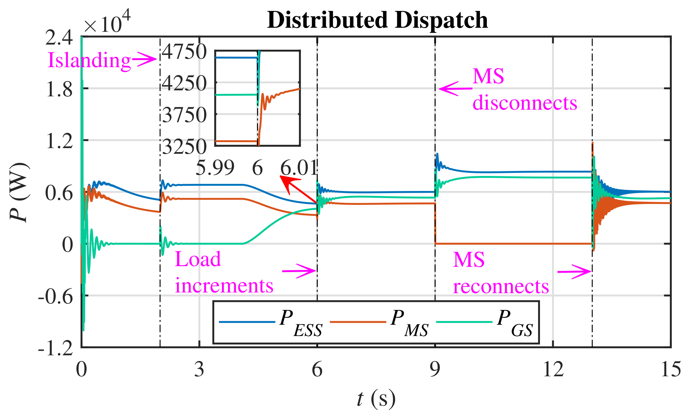
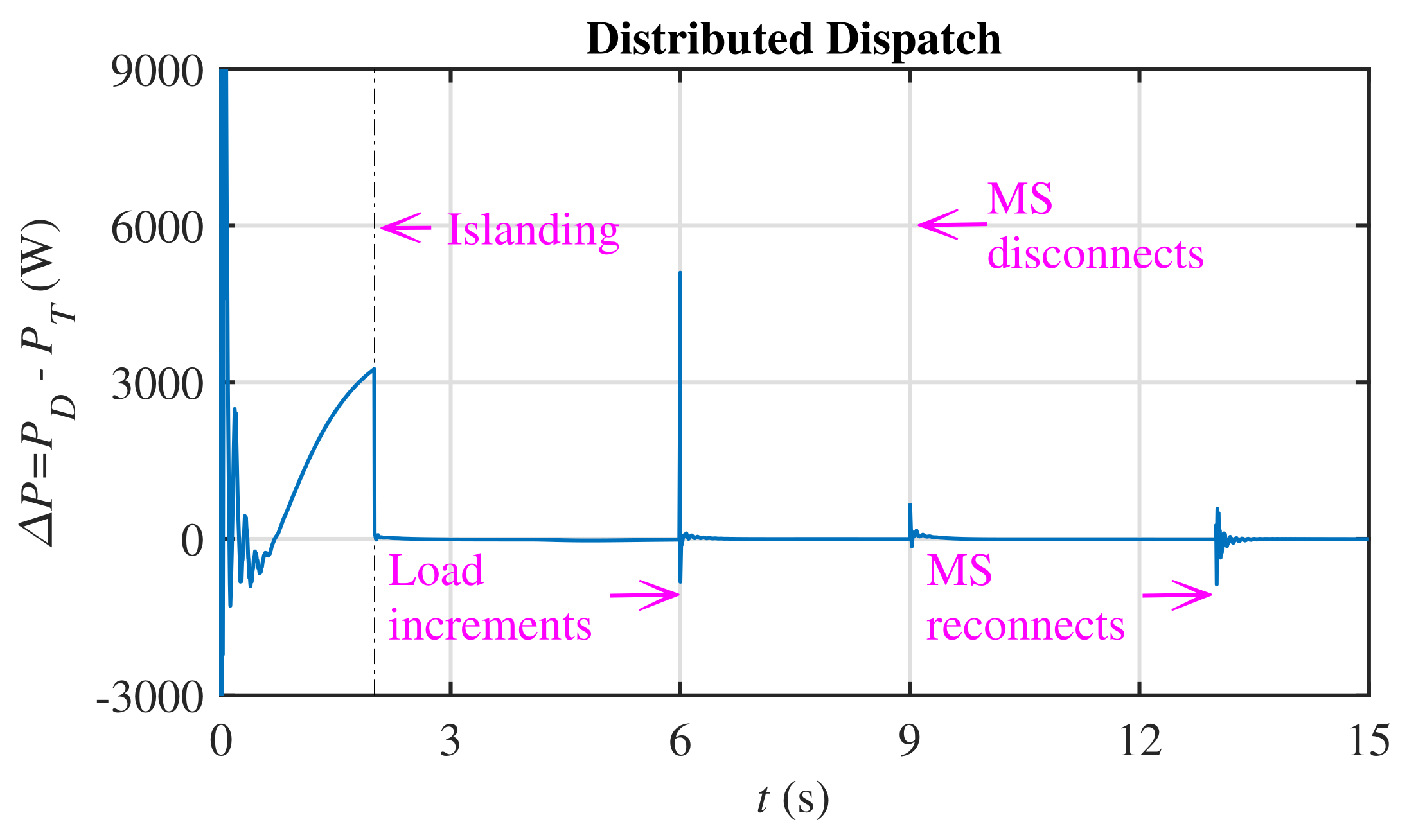
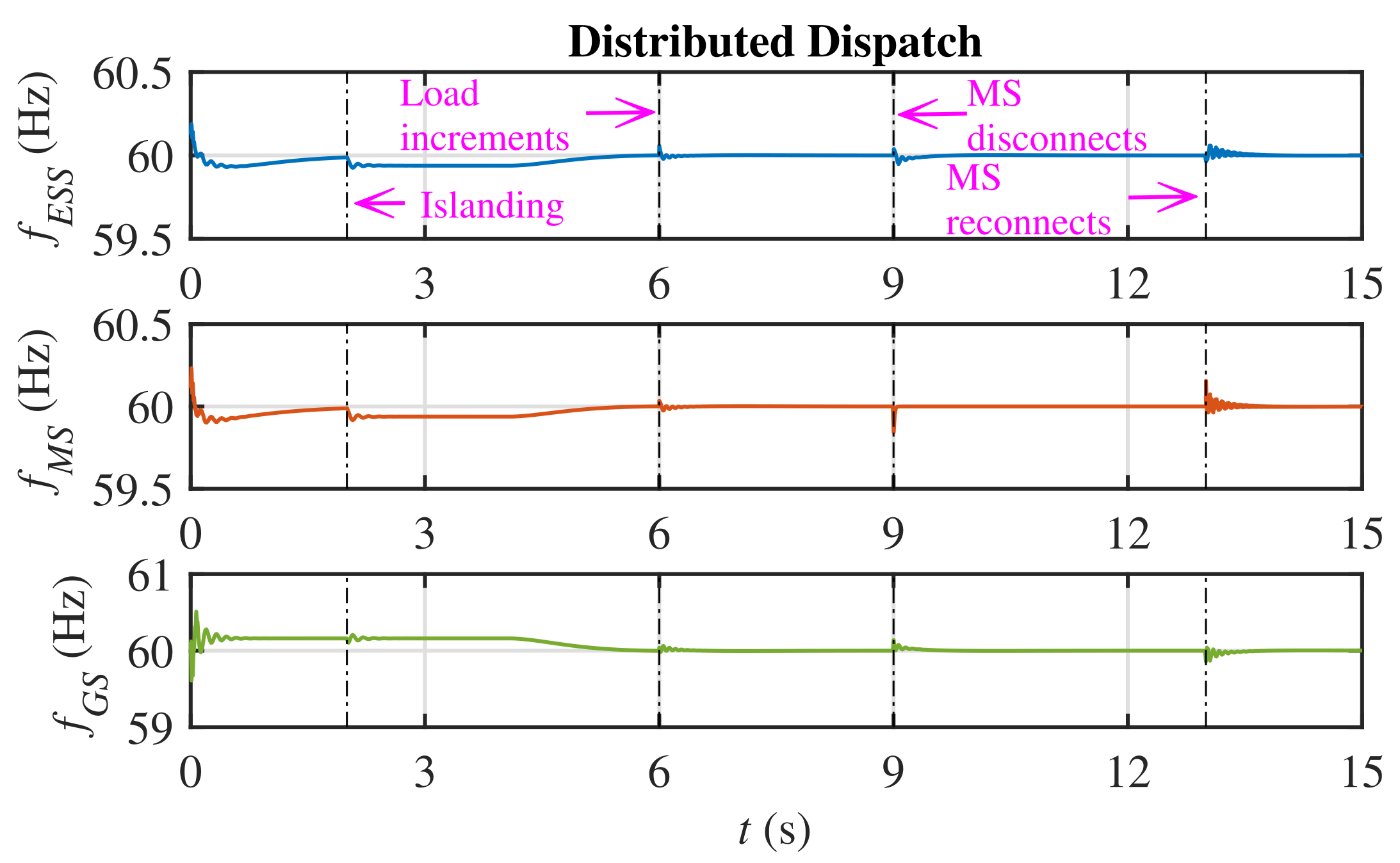
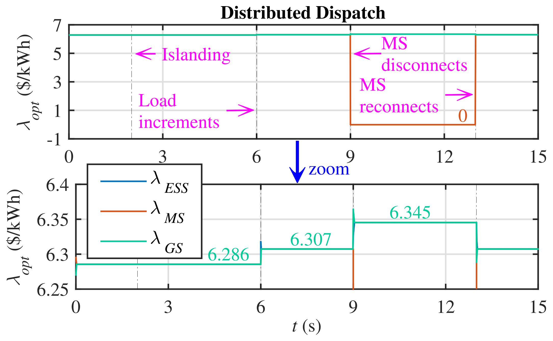
5.1. Case 1: Performance Assessment of the Proposed Hierarchical Control Framework for Distributed Economic Load Dispatch

In this case study, the microgrid is switched to the autonomous mode at $t=2 \mathrm{s}$. All the three control levels (i.e., primary, secondary and tertiary) are in place. The total active load power demand in the time interval $t\in$ [0,6] s is $P_D=12 \mathrm{k}\mathrm{W}$, which is then incremented to $P_D=16 \mathrm{k}\mathrm{W}$ in the time interval $t\in$ [6,9] s. The total demand then remains the same towards the end of simulation. However, in the interval $t\in$ [9,13] s one of the DGUs (i.e., MS) is plugged-out at $t=9 \mathrm{s}$ and, subsequently, plugged-in $t=13 \mathrm{s}$ for testing the plug-and-play feature of DGUs. The design parameters for the distributed secondary controller and distributed tertiary controller, expressed in Equations (7) and (17) are ${\kappa }_1,{\kappa }_2,\sigma =0.5$. Various generation cost related parameters of each DGU are specified in

Table 1. Cost parameters of the DGUs.

DGU Index (i)	Name of DGU	${\mathit{\alpha }}_{\mathit{i}}$	${\mathit{\beta }}_{\mathit{i}}$	${\mathit{\gamma }}_{\mathit{i}}$	${\mathit{P}}_{\mathbf{min}}\left(\mathbf{kW}\right)$	${\mathit{P}}_{\mathbf{max}}\left(\mathbf{kW}\right)$
1	ESS	180	6.21	0.0081	0	15
2	MS	200	6.23	0.0083	0	15
3	GS	190	6.22	0.0082	0	12.50

.

The overall closed-loop distributed hierarchical control scheme, as illustrated in Figure 2, operates as follows: the distributed tertiary controller generates the optimal power active dispatch references (i.e., $P_{i,opt}$) in a finite-time, and provides these to the distributed secondary controller. The distributed secondary controller tracks these stated references, generates new references (i.e., $P_{i,req}$), and provides these to the primary (i.e., $P\omega$-droop) controller of each DGU. In simple words, each higher control level commands the lower control level. As a result, not only is the power dispatched economically, but also the frequencies of DGUs are regulated to the reference value (i.e., $f_0=60\mathrm{Hz}$) in a finite-time, despite any load perturbation or the plug-and-play event of DGUs.

The optimal power dispatch references acquired by the distributed secondary controller from the distributed tertiary controller are depicted in Figure 5, and the corresponding power output of each DGU is shown in Figure 6. Since, the power mismatch, $\Delta P=P_D-P_T=P_D-{\sum }_{i=i}^N{P}_i$ (i.e., the difference between the overall active power demand and the combined active power output of the three DGUs), converges to zero, as shown in Figure 7, it implies that the distributed tertiary controller operates quite accurately. Moreover, the frequencies of DGUs are converging to the reference 60 $\mathrm{Hz}$, as illustrated in Figure 8. This in turn implies that the distributed secondary controller is quite accurately regulating the frequencies of DGUs under the load perturbation (i.e., $t\in [6,9]$ s) and the plug-and-play event (i.e., $t\in [9,13]$ s) of DGUs. The incremental costs of DGUs, ${\lambda }_{opt}$, and the corresponding total cost of generation, $C_T$, are given in Figure 9 and Figure 10 respectively. It can be seen that the incremental costs increase under the load increase and the plug-and-play events of DGUs. Similarly, the total cost of generation increases under the load increase event, but it decreases during the plug-and-play event, because of the disconnection of one DGU (i.e., MS) from a group of three.

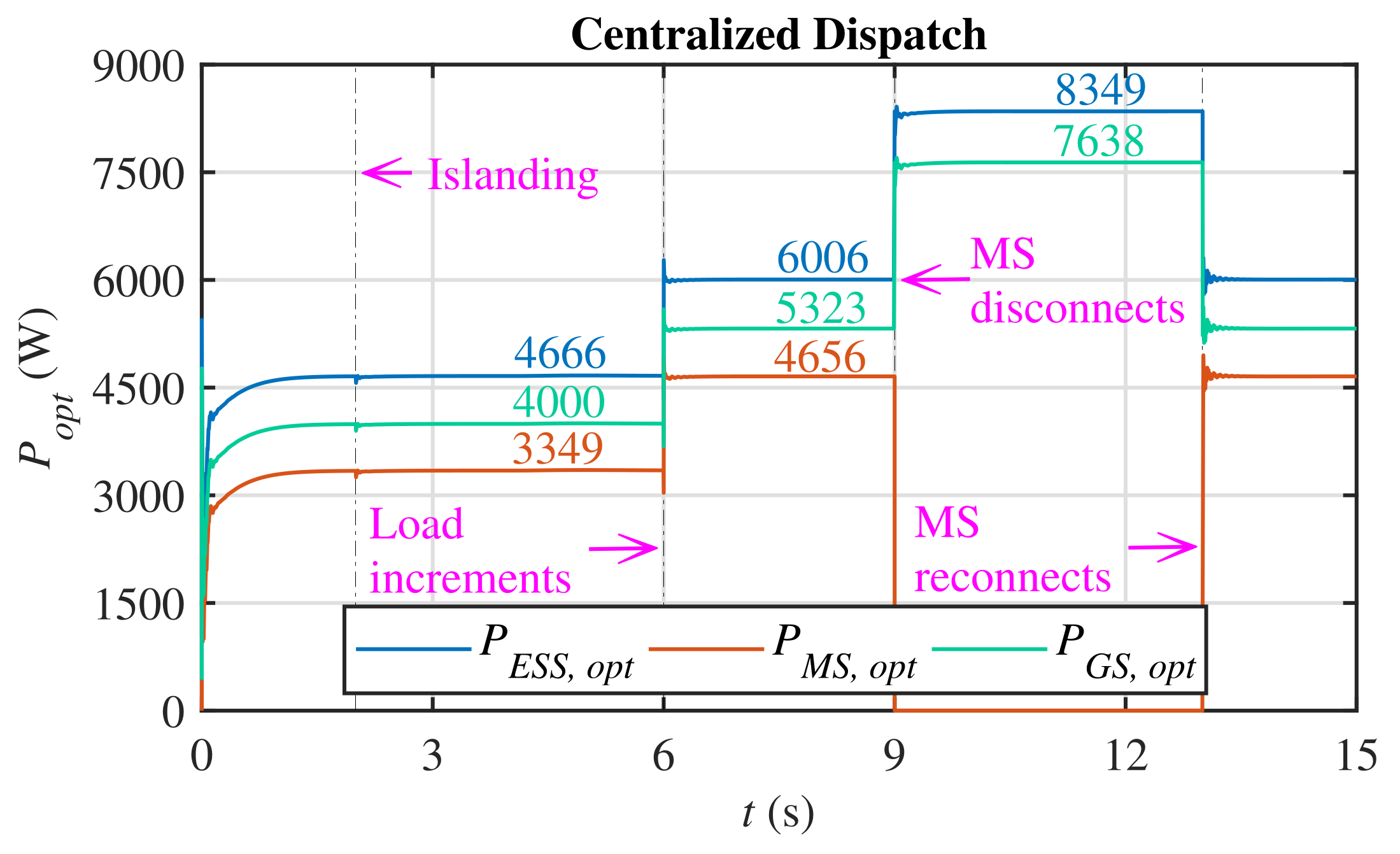
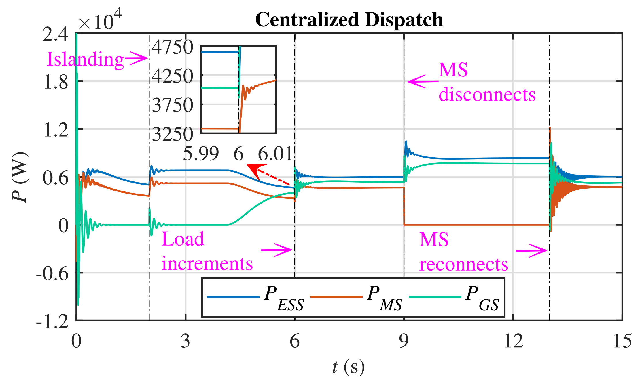
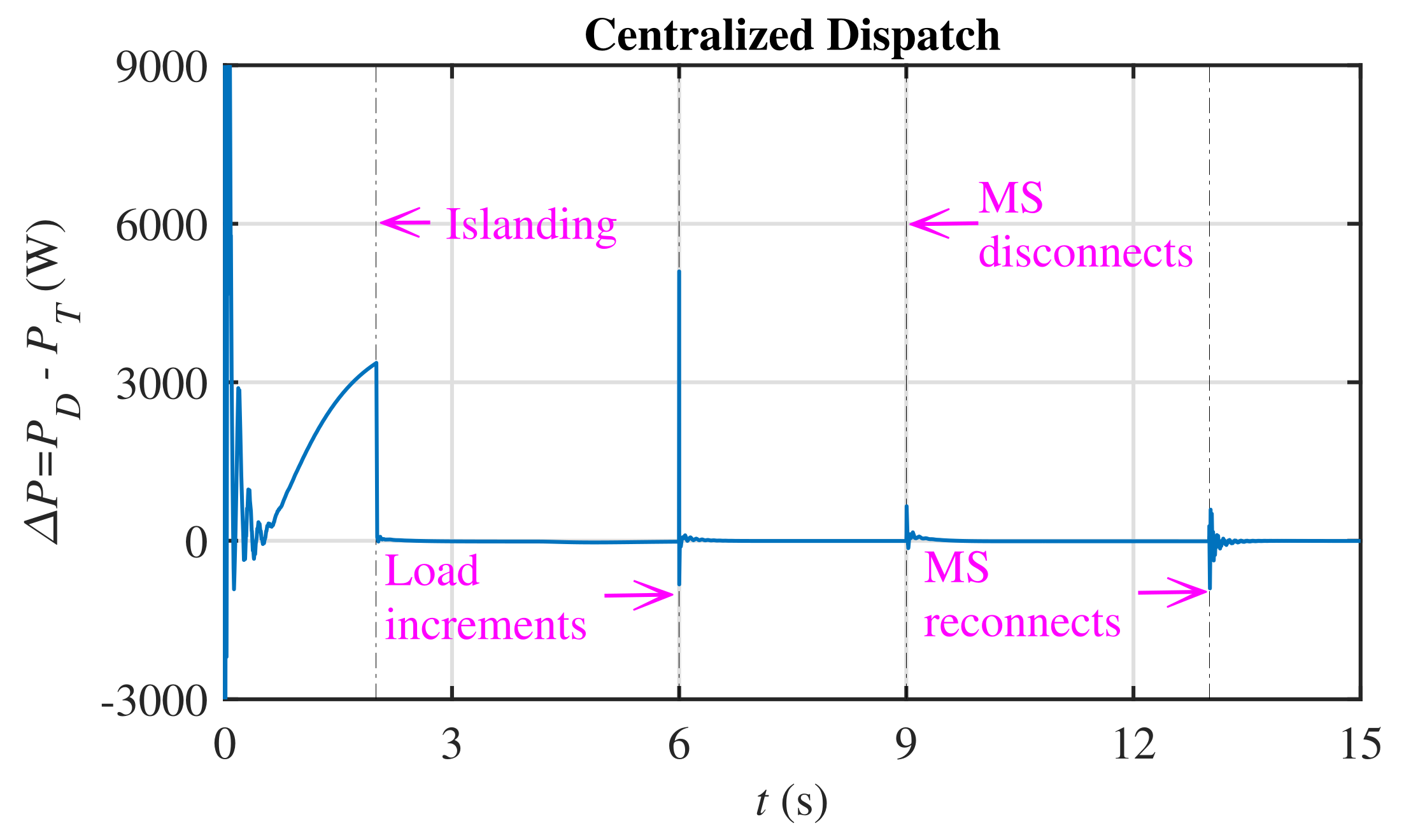
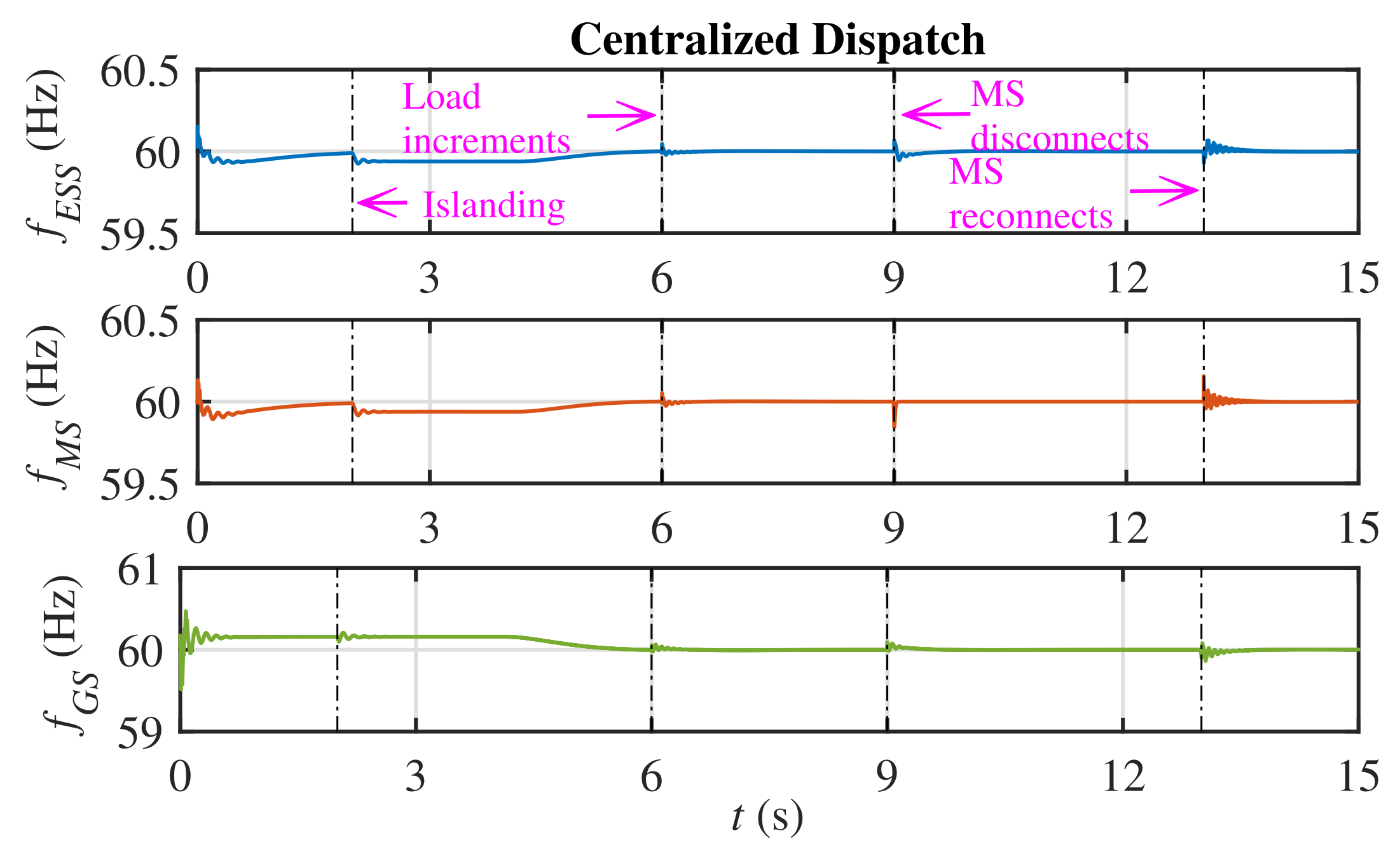
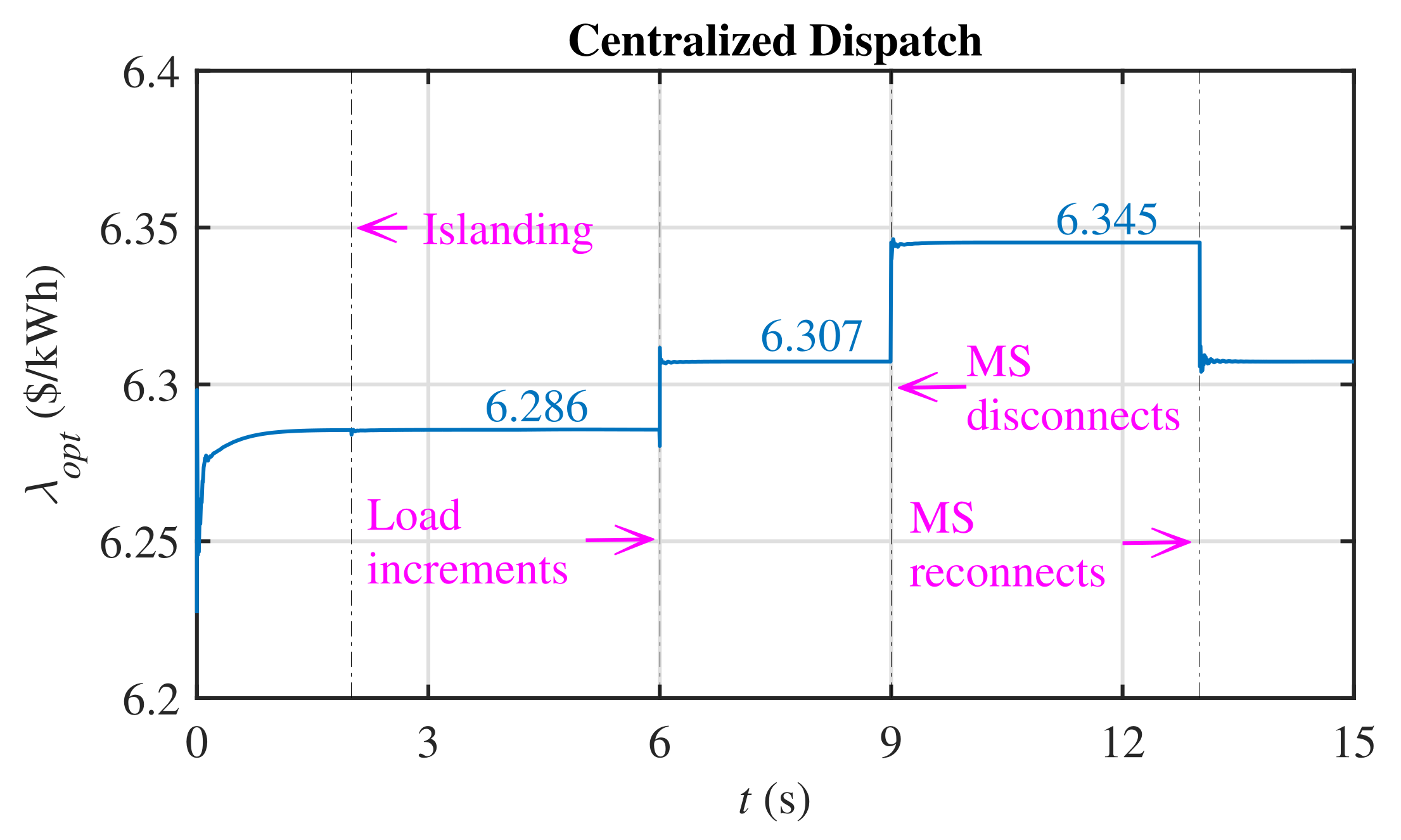
5.2. Case 2: Comparison with the Centralized Economic Load Dispatch

In this section, the proposed distributed economic dispatch strategy is further tested in comparison with the centralized economic dispatch strategy reported in well-known power system analysis and power generation, operation and control textbooks [44,45], and explained in Section 4.3.1.

In the centralized dispatch method, the optimal active power dispatch references acquired by the distributed secondary controller from the centralized tertiary controller are shown in Figure 11, and the corresponding power output of each DGU is depicted in Figure 12. It can be seen that both the optimal power dispatch references and the power outputs of DGUs under the proposed distributed economic dispatch, illustrated in Figure 5 and Figure 6, respectively, furnish approximately the same optimal solution as the centralized economic dispatch, shown in Figure 11 and Figure 12, respectively. The power mismatch, $\Delta P$, in the case of centralized dispatch, shown in Figure 13, likewise the distributed dispatch, shown in Figure 7, also converges to zero. Moreover, the frequencies of DGUs, the incremental costs of DGUs, and the total cost of generation under the centralized dispatch, shown in Figure 14, Figure 15 and Figure 16 are almost the same as those for the distributed economic dispatch, shown in Figure 8, Figure 9 and Figure 10, respectively. Please note that the proposed distributed economic dispatch strategy provides a comparable performance with the centralized economic dispatch strategy, but at a much lower cost of communication network. This makes the proposed distributed economic dispatch method a better solution than the centralized economic dispatch method.

6. Conclusions

In this paper, a fully distributed hierarchical control scheme is formulated for autonomous AC microgrids, comprising multiple DGUs with heterogeneous dynamics. The proposed scheme has a distinct three-layer control structure, comprising: primary control layer (based on traditional droop control); and leaderless consensus-based distributed secondary and tertiary control layers. The stated three layers work in a coordinated manner. The proposed strategy simultaneously regulates the frequency of each DGU to the reference value (i.e., 60 Hz) in a finite-time, and dispatches the load economically with a negligible power mismatch. It is pertinent to mention that the frequency restoration is achieved without requiring any central leader agent (i.e., leader–follower consensus) that has been reported in the contemporary distributed hierarchical control articles. Thus, the proposed strategy is insusceptible to the single point of failure due to the absence of leader. Moreover, the frequency restoration process does not need any dedicated auxiliary frequency control. Rather, the frequency restoration is achieved indirectly by regulating the active power output of each DGU at the secondary level. As compared to the conventional centralized hierarchical control, the proposed strategy only requires the local agent-to-agent information exchange through a sparse communication network, hence, it is fully distributed. The devised strategy is tested on an autonomous AC microgrid testbed, and found to successfully meet its targets under load perturbations, along with supporting the plug-and-play capability for DGUs. Detailed theoretical analysis and simulation results, performed in the MATLAB/Simulink environment, are presented to verify the effectiveness of the proposed control framework. Since, all the intended control objectives are successfully achieved, hence, the proposed distributed hierarchical control framework proves itself to be an effective technique for distributed economic dispatch and frequency regulation of an autonomous AC microgrid.

The present article deals only with the active power and frequency control of DGUs in an autonomous AC microgrid. The authors are determined to further this work by also considering the voltage and reactive power control and the associated virtual impedance concept. Similarly, the event-triggered communication mechanism can also be considered to increase the efficiency of the proposed control framework.

References

1. Lasseter, B. Microgrids [distributed power generation]. In Proceedings of the 2001 IEEE Power Engineering Society Winter Meeting (Conference Proceedings (Cat. No.01CH37194)), Columbus, OH, USA, 28 January–1 February 2001; pp. 146–149. [Google Scholar]
2. Lasseter, R.H. Microgrids. In Proceedings of the 2002 IEEE Power Engineering Society Winter Meeting (Conference Proceedings (Cat. No.02CH37309)), New York, NY, USA, 27–31 January 2002; pp. 305–308. [Google Scholar]
3. Lasseter, R.H.; Piagi, P. Microgrid: A conceptual solution. In Proceedings of the 2004 IEEE 35th Annual Power Electronics Specialists Conference (IEEE Cat. No. 04CH37551), Aachen, Germany, 20–25 June 2004; pp. 4285–4290. [Google Scholar]
4. Shi, W.; Li, N.; Chu, C.-C.; Gadh, R. Real-time energy management in microgrids. IEEE Trans. Smart Grid 2017, 8, 228–238. [Google Scholar] [CrossRef]
5. Dragicevic, T.; Wu, D.; Shafiee, Q.; Meng, L. Distributed and decentralized control architectures for converter-interfaced microgrids. Chin. J. Electr. Eng. 2017, 3, 41–52. [Google Scholar]
6. Moayedi, S.; Davoudi, A. Distributed tertiary control of DC microgrid clusters. IEEE Trans. Power Electron. 2017, 31, 1717–1733. [Google Scholar] [CrossRef]
7. United States Environmental Protection Agency. Distributed Generation of Electricity and Its Environmental Impacts. Available online: https://www.epa.gov/energy/distributed-generation-electricity-and-its-environmental-impacts (accessed on 22 June 2021).
8. Farrokhabadi, M.; Cañizares, C.A.; Simpson-Porco, J.W.; Nasr, E.; Fan, L. Microgrid stability definitions, analysis, and examples. IEEE Trans. Power Syst. 2019, 35, 13–29. [Google Scholar] [CrossRef]
9. IEEE 2030.7-2017—IEEE Standard for the Specification of Microgrid Controllers. Available online: https://ieeexplore.ieee.org/document/8340204 (accessed on 22 June 2021).
10. Bidram, A.; Davoudi, A. Hierarchical structure of microgrids control system. IEEE Trans. Smart Grid 2012, 3, 1963–1976. [Google Scholar] [CrossRef]
11. Bidram, A.; Lewis, F.L.; Davoudi, A. Distributed control systems for small-scale power networks: Using multiagent cooperative control theory. IEEE Control Syst. Mag. 2014, 34, 56–77. [Google Scholar]
12. Pilloni, A.; Pisano, A.; Usai, E. Robust finite-time frequency and voltage restoration of inverter-based microgrids via sliding-mode cooperative control. IEEE Trans. Ind. Electron. 2017, 65, 907–917. [Google Scholar] [CrossRef]
13. Bidram, A.; Davoudi, A.; Lewis, F.L.; Guerrero, J.M. Distributed cooperative secondary control of microgrids using feedback linearization. IEEE Trans. Power Syst. 2013, 28, 3462–3470. [Google Scholar] [CrossRef] [Green Version]
14. Guerrero, J.M.; Chandorkar, M.; Lee, T.-L.; Loh, P.C. Advanced control architectures for intelligent microgrids—Part I: Decentralized and hierarchical control. IEEE Trans. Ind. Electron. 2012, 60, 1254–1262. [Google Scholar] [CrossRef] [Green Version]
15. Baghaee, H.R.; Mirsalim, M.; Gharehpetian, G.B. Real-time verification of new controller to improve small/large-signal stability and fault ride-through capability of multi-DER microgrids. IET Gener. Transm. Distrib. 2016, 10, 3068–3084. [Google Scholar] [CrossRef]
16. Madurai Elavarasan, R.; Pugazhendhi, R.; Irfan, M.; Mihet-Popa, L.; Campana, P.E.; Khan, I.A. A novel Sustainable Development Goal 7 composite index as the paradigm for energy sustainability assessment: A case study from Europe. Appl. Energy 2021, 118173, in press. [Google Scholar] [CrossRef]
17. Madurai Elavarasan, R.; Leoponraj, S.; Dheeraj, A.; Irfan, M.; Gangaram Sundar, G.; Mahesh, G.K. PV-Diesel-Hydrogen fuel cell based grid connected configurations for an institutional building using BWM framework and cost optimization algorithm. Sustain. Energy Technol. Assess. 2021, 43, 100934. [Google Scholar] [CrossRef]
18. Nuvvula, R.S.S.; Devaraj, E.; Madurai Elavarasan, R.; Iman Taheri, S.; Irfan, M.; Teegala, K.S. Multi-objective mutation-enabled adaptive local attractor quantum behaved particle swarm optimisation based optimal sizing of hybrid renewable energy system for smart cities in India. Sustain. Energy Technol. Assess. 2022, 49, 101689. [Google Scholar] [CrossRef]
19. Dehkordi, N.M.; Sadati, N.; Hamzeh, M. Distributed robust finite-time secondary voltage and frequency control of islanded microgrids. IEEE Trans. Power Syst. 2016, 32, 3648–3659. [Google Scholar] [CrossRef]
20. Irfan, M.; Elavarasan, R.M.; Hao, Y.; Feng, M.; Sailan, D. An assessment of consumers’ willingness to utilize solar energy in China: End-users’ perspective. J. Cleaner Prod. 2021, 292, 126008. [Google Scholar] [CrossRef]
21. Irfan, M.; Hao, Y.; Ikram, M.; Wu, H.; Akram, R.; Rauf, A. Assessment of the public acceptance and utilization of renewable energy in Pakistan. Sustain. Prod. Consum. 2021, 27, 312–324. [Google Scholar] [CrossRef]
22. Dehkordi, N.M.; Baghaee, H.R.; Sadati, N.; Guerrero, J.M. Distributed noise-resilient secondary voltage and frequency control for islanded microgrids. IEEE Trans. Smart Grid 2018, 10, 3780–3790. [Google Scholar] [CrossRef] [Green Version]
23. Bidram, A.; Davoudi, A.; Lewis, F.L.; Ge, S.S. Distributed adaptive voltage control of inverter-based microgrids. IEEE Trans. Energy Convers. 2014, 29, 862–872. [Google Scholar] [CrossRef]
24. Bidram, A.; Davoudi, A.; Lewis, F.L.; Qu, Z. Secondary control of microgrids based on distributed cooperative control of multi-agent systems. IET Gener. Transm. Distrib. 2013, 7, 822–831. [Google Scholar] [CrossRef] [Green Version]
25. Hou, X.; Sun, Y.; Lu, J.; Zhang, X.; Koh, L.H.; Su, M.; Guerrero, J.M. Distributed hierarchical control of AC microgrid operating in grid-connected, islanded and their transition modes. IEEE Access 2018, 6, 77388–77401. [Google Scholar] [CrossRef]
26. Rey, J.M.; Vergara, P.P.; Castilla, M.; Camacho, A.; Velasco, M.; Martí, P. Droop-free hierarchical control strategy for inverter-based AC microgrids. IET Power Electron. 2020, 13, 1403–1415. [Google Scholar] [CrossRef]
27. Zhao, Z.; Yang, P.; Guerrero, J.M.; Xu, Z.; Green, T.C. Multiple-time-scales hierarchical frequency stability control strategy of medium-voltage isolated microgrid. IEEE Trans. Power Electron. 2016, 31, 5974–5991. [Google Scholar] [CrossRef]
28. Mehmood, F.; Khan, B.; Ali, S. Renewable generation intermittence and economic dispatch control of autonomous microgrid with distributed sliding mode. Int. J. Electr. Power Energy Syst. 2021, 130, 106937. [Google Scholar] [CrossRef]
29. Mehmood, F.; Khan, B.; Ali, S.M.; Rossiter, J.A. Distributed model predictive based secondary control for economic production and frequency regulation of MG. IET Control Theory Appl. 2019, 13, 2948–2958. [Google Scholar] [CrossRef]
30. Mehmood, F.; Khan, B.; Ali, S.M.; Rossiter, J.A. Distributed MPC for economic dispatch and intermittence control of renewable based autonomous microgrid. Electr. Power Syst. Res. 2021, 195, 107131. [Google Scholar] [CrossRef]
31. Wu, X.; Chen, L.; Shen, C.; Xu, Y.; He, J.; Fang, C. Distributed optimal operation of hierarchically controlled microgrids. ET Gener. Transm. Distrib. 2018, 12, 4142–4152. [Google Scholar] [CrossRef]
32. Li, Z.; Cheng, Z.; Liang, J.; Si, J.; Dong, L.; Li, S. Distributed event-triggered secondary control for economic dispatch and frequency restoration control of droop-controlled AC microgrids. IEEE Trans. Sustain. Energy 2019, 11, 1938–1950. [Google Scholar] [CrossRef]
33. Cheng, Z.; Li, Z.; Liang, J.; Si, J.; Dong, L.; Gao, J. Distributed coordination control strategy for multiple residential solar PV systems in distribution networks. Int. J. Electr. Power Energy Syst. 2020, 117, 105660. [Google Scholar] [CrossRef]
34. Wang, Y.; Mondal, S.; Satpathi, K.; Xu, Y.; Dasgupta, S.; Gupta, A. Multi-Agent Distributed Power Management of DC Shipboard Power Systems for Optimal Fuel Efficiency. IIEEE Trans. Transp. Electrif. 2021, 7, 3050–3061. [Google Scholar] [CrossRef]
35. Nguyen, T.L.; Wang, Y.; Tran, Q.T.; Caire, R.; Xu, Y.; Gavriluta, C. A Distributed Hierarchical control framework in Islanded microgrids and its agent-based design for cyber-physical implementations. IEEE Trans. Ind. Electron. 2021, 68, 9685–9695. [Google Scholar] [CrossRef]
36. Dewadasa, M.; Ghosh, A.; Ledwich, G. Dynamic response of distributed generators in a hybrid microgrid. In Proceedings of the 2011 IEEE Power and Energy Society General Meeting, Detroit, MI, USA, 24–28 July 2011; pp. 1–8. [Google Scholar]
37. Ullah, S.; Khan, L.; Sami, I.; Ullah, N. Consensus-Based Delay-Tolerant Distributed Secondary Control Strategy for Droop Controlled AC Microgrids. IEEE Access 2021, 9, 6033–6049. [Google Scholar] [CrossRef]
38. Ullah, S.; Khan, L.; Badar, R.; Ullah, A.; Karam, F.W.; Khan, Z.A.; Rehman, A.U. Consensus based SoC trajectory tracking control design for economic-dispatched distributed battery energy storage system. PLoS ONE 2020, 15, e0232638. [Google Scholar] [CrossRef] [PubMed]
39. Erickson, M.J.; Lasseter, R.H. Integration of battery energy storage element in a CERTS microgrid. In Proceedings of the 2010 IEEE Energy Conversion Congress and Exposition, Atlanta, GA, USA, 12–16 September 2010; pp. 2570–2577. [Google Scholar]
40. Lasseter, R.H.; Piagi, P. Control and Design of Microgrid Components; Power Systems Engineering Research Center (PSERC), University of Wisconsin-Madison: Madison, WI, USA, 2006. Available online: https://certs.lbl.gov/sites/all/files/ctrl-design-microgrid-components.pdf (accessed on 20 October 2020).
41. Ullah, S.; Khan, L.; Jamil, M.; Jafar, M.; Mumtaz, S.; Ahmad, S. A Finite-Time Robust Distributed Cooperative Secondary Control Protocol for Droop-Based Islanded AC Microgrids. Energies 2021, 14, 2936. [Google Scholar] [CrossRef]
42. Chen, F.; Cao, Y.; Ren, W. Distributed average tracking of multiple time-varying reference signals with bounded derivatives. IEEE Trans. Autom. Control 2012, 57, 3169–3174. [Google Scholar] [CrossRef]
43. Cortes, J. Discontinuous dynamical systems. IEEE Control Syst. Mag. 2008, 28, 36–73. [Google Scholar]
44. Saadat, H. Power System Analysis, 3rd ed.; PSA Publishing: Williamsport, PA, USA, 2010. [Google Scholar]
45. Wood, A.J.; Wollenberg, B.F.; Sheblé, G.B. Power Generation, Operation, and Control; Wiley: Hoboken, NJ, USA, 2013. [Google Scholar]
46. Liu, X.; Lam, J.; Yu, W.; Chen, G. Finite-time consensus of multiagent systems with a switching protocol. IEEE Trans. Neural Netw. Learn. Syst. 2015, 27, 853–862. [Google Scholar] [CrossRef]
47. Zuo, Z.; Tie, L. Distributed robust finite-time nonlinear consensus protocols for multi-agent systems. Int. J. Syst. Sci. 2016, 47, 1366–1375. [Google Scholar] [CrossRef]
48. Zhang, H.; Lewis, F.L.; Qu, Z. Lyapunov, adaptive, and optimal design techniques for cooperative systems on directed communication graphs. IEEE Trans. Ind. Electron. 2012, 59, 3026–3041. [Google Scholar] [CrossRef]
49. Bhat, S.P.; Bernstein, D.S. Finite-time stability of continuous autonomous systems. SIAM J. Control Optim. 2000, 38, 751–766. [Google Scholar] [CrossRef]
Figure 1. Microgrid simulation testbed and undirected communication graph between DGUs. (a) Microgrid simulation testbed.; (b) Communication graph.
Energies 14 08408 g001
Figure 2. Overall closed-loop implementation of the proposed distributed hierarchical control framework.
Energies 14 08408 g002
Figure 3. Primary control strategy for inverter-interfaced DGUs (i.e., ESS and MS).
Energies 14 08408 g003
Figure 4. Primary control strategy for ICE-based DGU (i.e., diesel GS).
Energies 14 08408 g004
Figure 5. The optimal power dispatch references for DGUs.
Energies 14 08408 g005
Figure 6. Power outputs of DGUs.
Energies 14 08408 g006
Figure 7. Power mismatch.
Energies 14 08408 g007
Figure 8. Frequencies of DGUs.
Energies 14 08408 g008
Figure 9. Incremental costs of DGUs.
Energies 14 08408 g009
Figure 10. Total generation cost of DGUs.
Energies 14 08408 g010
Figure 11. The optimal power dispatch references for DGUs.
Energies 14 08408 g011
Figure 12. Power outputs of DGUs.
Energies 14 08408 g012
Figure 13. Power mismatch.
Energies 14 08408 g013
Figure 14. Frequencies of DGUs.
Energies 14 08408 g014
Figure 15. Incremental costs of DGUs.
Energies 14 08408 g015
Figure 16. Total generation cost of DGUs.
Energies 14 08408 g016