PV-Supercapacitor Cascaded Topology for Primary Frequency Responses and Dynamic Inertia Emulation

Abstract

Owing to rapid increase in PV penetration without inherent inertia, there has been an unremitting deterioration of the effective inertia of the existing power systems. This may pose a serious threat to the stability of power systems during disturbances if not taken care of. Hence, the problem of how to emulate Synthetic Inertia (SI) in PV Systems (PVS) to retain their frequency stability demands attention. Super Capacitor (SC)-based storage become an attractive option over the other energy storage types because of its high-power density, burst power handling capability, faster response and longer life cycle. Considering this, the authors here propose a novel PV-SC Cascaded Topology (PSCT) as a cost-effective approach to emulate SI by integrating a low voltage SC to a high voltage grid-connected PVS. The proposed PSCT helps in operating the SC as a voltage source rather than a current source. Thus, it eliminates the high gain requirements of the SC interfacing converters. The aim is to target two main frequency response services, i.e., Primary Frequency Response (PFR) and Synthetic Inertial Response (SIR), using a novel common control scheme, but without affecting any other energy intensive services. The authors introduced a Droop-Inspired (DI) method with an adjustable inertia constant to emulate dynamic inertia so that a wider range of Rate of Change of Frequency (RoCoF) values can be serviced with a limited storage. A very streamlined analysis was also carried out for sizing of the SC stage based on a simple Three-Point Linearization (TPL) technique and DI technique with a limited knowledge of the disturbance parameters. The whole system was initially validated in a MATLAB Simulink environment and later confirmed with the OPAL-RT Real-Time Simulator. The investigated response was subject to variation in terms of control parameters, changes in solar irradiance, grid frequency variation, etc.

1. Introduction

In light of increased PV penetration [1,2,3], it is necessary to analyze the requirements and challenges that existing power systems will face in near future. Degradation of transient stability and/or declining equivalent inertia of the power system is one of the major concerns [4,5,6]. Due to lack of the inherent energy buffering capability in the case of power electronics-based PVS, as there are no physical rotating parts unlike classical thermal power generators, the effective inertia of the power grid is on the decline. This issue may lead to situations that can ultimately destabilize the power grid under extreme conditions. It is estimated that by the end of 2022, there will be a noticeable reduction in the equivalent inertia of power systems by up to 25% if proper measures are not taken [4]. Any mismatch between the generated active power and the sporadic load demand can trigger frequency deviation and, in turn, large power swings; this could degrade the performance of the system. Low inertia systems will experience faster changes in frequency, which will lead to the false triggering of various protective relays in order to trip the DGs, which operate with a strict frequency band. This will, in turn, activate the load-shedding controllers, which will further worsen the situation, initiating a chain reaction. This situation may bring down the resilience of the power system even to small disturbances, and could trip a whole grid, which would result in complete blackout unless otherwise protected.

Several such cases have been reported in various parts of world in the recent past. In 2011, one such incident was experienced by the power system of the Northern Island of New Zealand, when the frequency nadir reached as low as 47.5 Hz with a severe RoCoF of 0.73 Hz/s [4]. A similar incident happened in Hawaii with a RoCoF of 0.373 Hz/s resulting in back-to-back chain tripping of several DGs [4]. Another such incident was reported in the Island of Cyprus in January 2012, and, in this case, the reason was severe RoCoF [5]. Recently, in 2019, the renewable reach of the UK grid also experienced a frequency nadir ($f_{nadir}$) of 49.1 Hz due to the disconnection of about 350 MW of DGs from the parent grid, causing more than one million consumers to suffer [6]. In view of this, it is essential for the PV systems to emulate inertial characteristics such as those of state-of-the-art synchronous generators. This contingent measure is highly essential in order to avoid the very real possibility of larger-scale future grid catastrophes. The concept of SI was actually derived from the ac micro-grids, which mostly suffer from the zero or low rotational inertia problem as most of the power sources are converter/inverter-based power electronics. Therefore, in order to behave as a virtual synchronous generator, it is recommended for the PV either to operate away from MPPT or to have some kind of energy storage while feeding power to the network. In this way, during grid disturbances, this storage can mimic the behavior of the actual rotational inertia to make the system stable, self-sustainable and more grid-friendly.

Many works have been cited in the literature that show the utilization of some kind of virtual or actual energy storage to emulate SI for the PVS by means of converter/inverter dynamics. These are mainly divided into two categories: Actual Storage-based and Virtual Storage-based. Both approaches have their own advantages and disadvantages and are reviewed in detail. In [7,8,9,10,11,12], the authors explored the use of a Battery Energy Storage System (BESS) to mimic the inertial response for PVS for different frequency event scenarios. In [7], distributed ESS are studied for a large PVS using a coordinated central control scheme. However, in [8,9], the target was to optimize the lumped storage size and its life cycle, with an appropriate degree of control, for an islanded micro grid. In [10], the authors tried to find out the optimal location of the lumped storage while taking into account the contingency of future blackouts and the severity of the stochastic PV penetration level. Some revenue-optimization control methods are presented in [11,12], where the BESS is used for both PFC as well as load shifting while optimizing the size of the storage. However, the adverse effect of the high ramping rate on the SOC and the lifespan of the BESS are not considered in both cases.

However, the use of BESS being the early approach towards frequency regulation certainly compromises between the ramp rate and the lifespan of the battery due to low power density. To address the issue of low ramp rate, the authors of [13] explored the use of a flywheel as a hybrid storage approach to BESS that became less popular due to its larger footprint. Alternatively, a few authors [14,15,16] also explored the concept of Super Conductive Magnetic Energy Storage (SMES) due to its burst power handling capability, rapid response time, high power density, and high efficiency compared to BESS, while targeting several power quality issues. However, major disadvantages such as the lager footprint of the coil for high power applications, the high running cost for maintaining the superconducting critical temperature, and the high material cost of the coil, make it unrealistic.

Recently, the concept of virtual energy storage approaches has drawn the attention of the research community as an effective solution towards the low lifespan of the BESS involving the mimicking of virtual inertia in PVS to improve the frequency nadir. One such approach is the PV reserve method, also known as PV delta power control [17] or PV deloaded control [18,19,20,21,22]. The operating mechanisms of both the methods are quite similar. In the former case, a major part of the installed PV modules is operated in MPPT mode, whereas a few modules are intentionally kept ideal or operated away from MPPT. However, in the latter case, the whole PV installation is operated in OFF MMPT mode. In [23], the authors presented the concept of dynamic inertia emulation for PVS using the PV reserve method. The concern was that during the peak sun hour time, the power grid experiences a considerable fall in system inertia as the contribution is more from PV than the classical thermal generators. To achieve this, a neuro-fuzzy logic control-based self-adoptive algorithm is presented in [23]. This modifies the PV reserve capacity based on the time-dependent generation and load demand to improve the system’s response to frequency events, while optimizing the utilization of the installed PV capacity. The authors of [24,25] proposed a similar approach as well, where a dynamic droop coefficient-based droop control technique was used in [24] to emulate variable inertia support during frequency events. Nevertheless, this approach goes through a lot of power oscillation, as the complex control technique demands a proper tuning of its coefficients. In [25], the authors implemented a complex self-adoptive fuzzy logic method to emulate virtual inertia to improve the frequency stability. However, in both studies, the proposed controls were the main concern, but the targeted energy storage types were undisclosed.

Though the PV reserve method sounds interesting, there are a few disadvantages of PV reserve methods over BESS, which certainly cannot be ignored. Firstly, it has a larger footprint, and lower power and energy density, as compared to BESS. Secondly, the former method is mostly uneconomical in terms of both fixed and running costs, as the PV system is under-utilized throughout the running time even though there are no frequency events. Thirdly, it is highly uncertain how PV will support the required power to emulate the frequency response during low-insolation and night-time periods. Recently, another virtual energy storage-based approach gained popularity in terms of addressing the issues with the PV reserve-type approach. The authors of [26,27,28] tried to utilize the electrostatic energy of the DC-link capacitor to emulate virtual inertia during frequency events. Conversely, this approach was limited only to low power applications because of the low energy density of the DC-link capacitors and high fluctuation in DC-link voltage. Instead, a large capacitor can manage the work but will result in a larger footprint, higher costs and larger start-up times due to its slow dynamics [29].

In view of all these issues, the electric double layer capacitor (ELDC), also known as the Super Capacitor (SC) or ultra-capacitor, has recently, become more popular owing to its high power and energy bursting capability, which are similar to SMES. At the same time, it has, comparatively speaking, a much smaller footprint than SMES, excellent efficiency (greater than 95%) and a long and maintenance-free life cycle compared to BESS (more than 30 years), and has a steadily improving benefit-to-cost ratio relative to SMES and Flywheel-type storage [30]. There are several articles that have given emphasis to SC-based energy storage systems for grid quality improvement in PVS. Yet, as SC has comparatively low energy density than BESS, most of the approaches involve hybrid energy-based storages such as BESS with SC [31], fuel cell with SC [32], etc. In these approaches, the transient and the steady state power and/or energy sharing between the storage types were decided by the proposed coordinated control. The hybrid storage concepts were found to be more successful when the target not only provided frequency support but also high-energy intensive services such as load shifting and peak saving. Thus, these approaches optimize costs by improving the utilization factor and lifetime of the storage systems. However, the hybrid storage concept seems to be a costly affair when only the frequency support activities are targeted. In this paper, the focus lies in the most simple and economic solution for frequency services in PVS, which is better achieved by employing SCs.

In [30,33], a low voltage DC-link was considered for the inverter and the corresponding DC-link was replaced by an SC/ELDC to target PV generation smoothing. However, this demanded a larger SC for a specific energy requirement, as it was not possible to discharge the DC-link capacitor beyond a certain limit in order for the inverter to function. This resulted in higher costs and the SC was also underutilized. However, there are many other studies that also use a larger SC to avoid the gain requirement of the interfacing converters [31,32,34,35,36,37,38] for different applications in DC/AC micro grids. To avoid the need for an additional converter for use in the charge control function, many articles [38,39,40,41] have proposed various isolated or non-isolated multiport converter topologies as well to interface energy storage for the PVS. However, most of these isolated topologies, if used for the integration of SC, will suffer from gain problems related to high voltage and current stresses due to large variations in SC voltage. However, in some of the cases [41,42,43], irrespective of isolated or non-isolated type of topology, the system configuration does not allow the integration of low voltage energy storage to the PVS. In [44], a switch capacitor-derived multiport converter was proposed to integrate a low voltage storage to the PVS; however, the same could not be suggested for the integration of SC, because, in cases in which switched capacitor-derived converters are used, the efficiency drops severely when the voltage gain moves away from the fixed nominal value. The authors of [45,46,47] proposed various series cascaded topologies based on the fractional power processing concept to integrate energy storage; however, the power process capability of the storage was strictly limited by the voltage difference between the input and output port voltage of the converter. Moreover, the interfacing converter must be a very high-gain converter although it processes partial power. Apart from that, the existing cascaded topologies have serious fault-tolerance limitations due to their use of series configurations, and these issues certainly cannot be ignored.

In consideration of all the aforementioned issues, in this paper, the advantages of SC are used as a basis to provide frequency response services to medium-voltage-level PVS in order to showcase how this hybridization benefits the conventional widely adopted grid type when control is applied in terms of frequency support. There are many studies that also focus on the concept of Virtual Synchronous Machine (VSM) [48] and Grid-Forming Control (GFC), which is indeed the future of PV systems; however, GFM control is not the focus of this particular paper. This proposed approach has the capability of covering a wide range of power applications stretching from those involving a few kilowatts to larger applications operating at the power level of hundreds of kilowatts. The aim is to address some of the services that are ancillary to the frequency response, such as SIR and PFR activities, etc., but not to target any other high-energy intensive services such as load shifting, peak saving, etc. due to the limited storage capacity. The novel contributions of the paper are outlined below for the reader’s convenience:

• Topological innovation: The proposed “PV-SC Series Cascade Topology” represents a pioneering approach to interface a low-voltage SC to a medium-/high-voltage PVS, which, unlike its counterparts, eliminates the need for a high gain complex isolated converter for the SC Power-Processing Stage (SC-PPS).
• Innovation in Control: Firstly, the proposed “Droop Inspired” method offers a means of emulating dynamic inertia as a function RoCoF. The target is to serve a wider range of RoCoF with a limited storage. Secondly, the novel single PI controller-based decoupling method effectively segregates the control of two-level SC-PPS in order to operate the SC as a voltage source rather than as a current source. A combined control scheme is also used to address both the SIR and the PFR.
• Innovation in methodology for sizing: A very simple approach is proposed for the sizing of the SC and its PPS using a novel “Three Point Linearization” method for the PFR and the “Droop Inspired” method for the SIR.

The paper is organized into the following sections. Section 2 details the working principle of the proposed PSCT. A brief explanation of the frequency response activities is given, and this is followed by a discussion of the proposed DI-method-based dynamic inertia concept in Section 3. In Section 4, the implemented control schemes are discussed to in terms of the degree to which they fulfil their objectives. In Section 5 the sizing of the SC-based storage is covered based on the proposed DI and TPL methods. The whole concept is verified in Section 6 for various case studies, using MATLAB Simulink, and then validated using the OPAL-RT-based real-time simulator. Finally, Section 7 offers conclusions regarding the issues discussed in the paper.

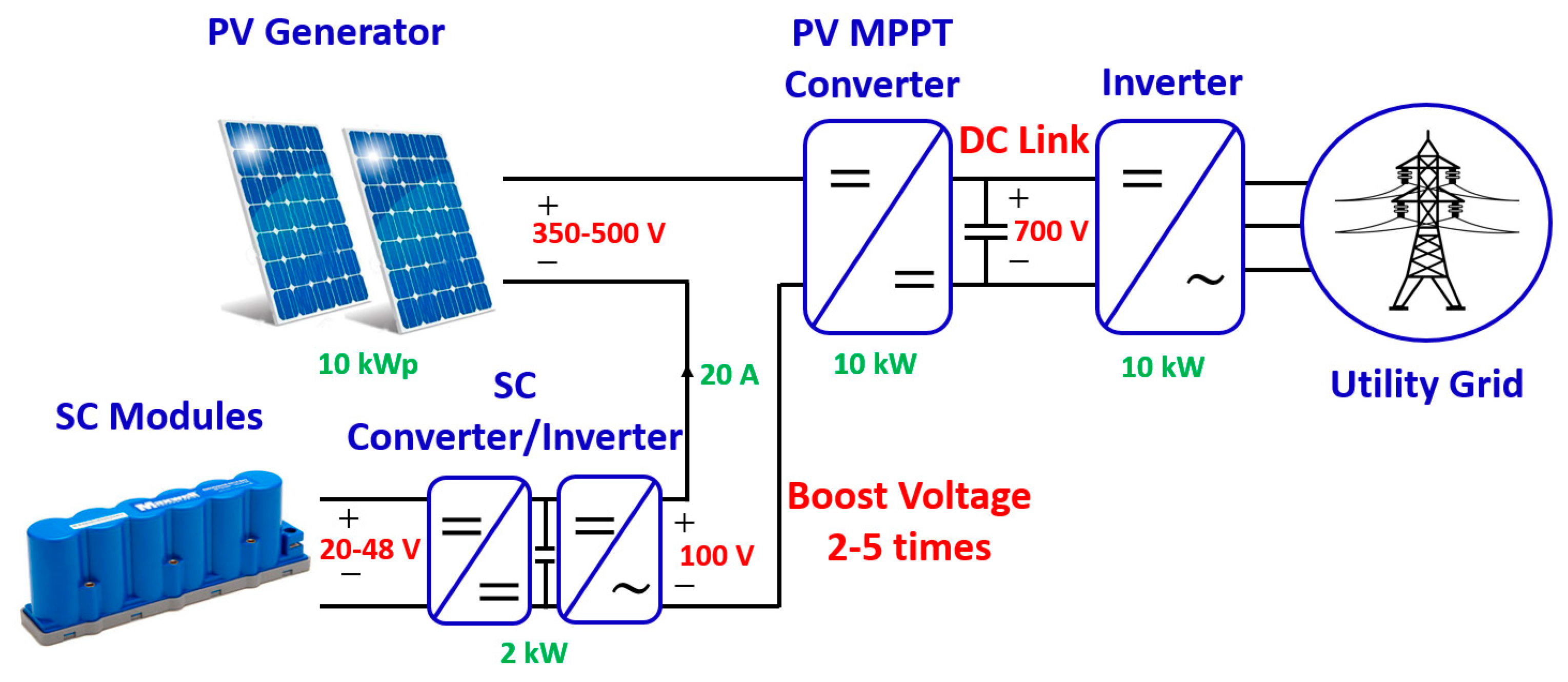
2. Proposed PV-SC Series Cascaded Topology

2.1. System under Consideration

Recently, the Indian government expressed that they aim to install 100 GW of solar power infrastructure by the end of 2022, of which around 40 GW is anticipated to come from rooftop solar installations [2]. In addition, after signing the Paris Agreement in 2015 [3], India has committed to a long-term target of acquiring 40% of its electricity generation from non-conventional sources by 2030. Keeping this in mind, the authors of this study attempted address the medium to high power level PVS systems with built-in inertia emulation capabilities for use in grid-supporting activities such as SIR and PFR, etc., where the application ranges from string inverter topologies of a few kilowatts PV to multi-string inverter topologies operating at hundreds of kilowatts PV. The authors found that a 5:1 combination of the PV and SC power rating may be the best solution to address the objectives, and this is confirmed in Section 5. Hence, a 10 kWp PVS with 2 kW SC-PPS was taken into consideration by the authors as a base model, which, in turn, could be extended to any high-power level when taking into account modularity. The detailed ratings and specifications for the PV, SC, DC-link and the inverter/converter stages are given in

Table 1. System under consideration for the proposed PSCT.

System/Parameters	Ratings
PV capacity at STC	10 kWp, 500 V, 20 Amps
Grid parameters	Three Phase, 400 V rms, 50 Hz
SC storage capacity	22 kJ, 19.33 F, 48 V, 170 Amps (peak)
DC link voltage	700 V (Regulated)
Boost Converter for MPPT	10 kW, Input voltage (300 to 700), Output voltage 700 V
Three-phase two-level grid-connected VSI	10 kVA, 700 V DC, 400 V (L-L) rms, 50 Hz
SC charge controller	2 kW, 48 V, 100 Amps

.

Considering the required specifications listed in Table 1, the basic configurational idea that comes to mind is to integrate the SC to the DC-link of the PVS in a parallel fashion using a high-gain converter, as shown in Figure 1. Nevertheless, as the aim is to utilize the SC energy fully (in practical terms, around 80% of its rated energy), the gain demand of the interfacing converter can be sky high during periods of low SOC levels for the SC, which is definitely a matter of concern. This actually motivated the authors to come up with a solution to interface the SC as a series element to the PV using some extremely low-gain converters. In this way, the SOC can be controlled by operating the SC as a voltage source rather than a current source by injecting a series bipolar voltage of the required variable magnitude to the PV voltage.

The proposed PSCT is shown in Figure 2 and the corresponding SC-PPS of the proposed converter is shown in Figure 3 for a better visualization. As can be seen, it consists of a bidirectional buck-boost DC–DC converter followed by a Semi-Controlled Inverter (SCI). The DC–DC stage is used for boosting operations, whereas the SCI stage is a polarity changer and is sometimes used for bucking the output of the DC-DC stage if required. As the output of the SCI is connected in series with PV with the help of a smoothing LC filter, the current is always unidirectional and is the same as the PV current. Therefore, by simply inverting the polarity of the output voltage and by regulating its magnitude, we can actually charge and discharge the SC at a specific rate. As shown in Figure 2, an additional boost converter decouples the PV MPPT operation not only from the SC charge control operation but also from the grid-side operation of the inverter.

For the SC Buck-Boost stage, the Zig-Zag Boost (ZZB) bidirectional converter is used as a better alternative over the conventional Boost converter due to its better efficiency vs. gain characteristics and gain vs. duty cycle as compared to the conventional boost converters [49]. Secondly, the proposed converter can also meet the voltage gain requirement, which sometimes approaches a value of four, where the conventional boost converter fails or suffers from issues related to extremely low efficiency. The switches S1 and S2 of the ZZB are simultaneously turned ON or OFF, whereas the switch S3 is the complementary switch. The power flow direction of the ZZB can be decided by the direction of the current in the inductors L1 and L2. The PWM technique for the discharging and charging of the SC, and the corresponding modes of operation, are shown in Figure 4 and Figure 5, respectively. However, a thorough analysis and working principle of the proposed ZZB converter has already been published in [49], and hence, will not be covered in detail here. The SCI stage for SC is a simple H-bridge structure with two controlled and two uncontrolled switches. Here, the reason for using an SCI is due to the unidirectional nature of the current flow at its output, as the PV current cannot be negative. The SCI can be operated either in the unipolar or in the bipolar PWM mode of operation. In the bipolar mode of operation, the switches S4 and S5 are fired simultaneously, whereas, in case of the unipolar PWM mode of operation, the switches can be fired with a phase shift of 180°. The magnitude and polarity of its output voltage are decided based on the duration of duty cycle D. For the sake of understanding, the bipolar PWM technique with three modes of operation, as per the duration of D, are shown in Figure 6a–c, respectively. For 0 ≤ D < 0.5, the filtered output voltage of the SCI is negative, for 0.5 < D ≤ 1, the filtered output voltage is positive, and for D = 0.5, the filtered output voltage will be zero. The detailed control of both power-processing stages of the SC will be covered in Section 5.

2.2. Merits and Limitations of the Proposed PSCT in Terms of Fault Tolerance

This subsection covers a detailed comparative analysis of the proposed PSCT over the conventional series- and parallel-type topologies to highlight both its merits and its limitations. However, unlike the family of conventional cascaded topologies, the proposed PSCT has much more fault-tolerant capability either due to its inherent nature or by applying appropriate control or modification. Both the fault-tolerant capabilities and the limitations are specified below for better insight.

• Fault-tolerant capabilities:
  • As with other cascaded topologies, the proposed configuration is also prone to short circuit faults. However, a proper current regulation technique can set a current limit in the inner current loop control of the SC-PPS. Fortunately, as the PV array operates directly in series with the output port of the SC-PPS, any current beyond the short circuit current rating of the PV array will shift the PV characteristics to second quadrant, and thus, will activate the bypass diodes of the PV modules to save it from possible damage.
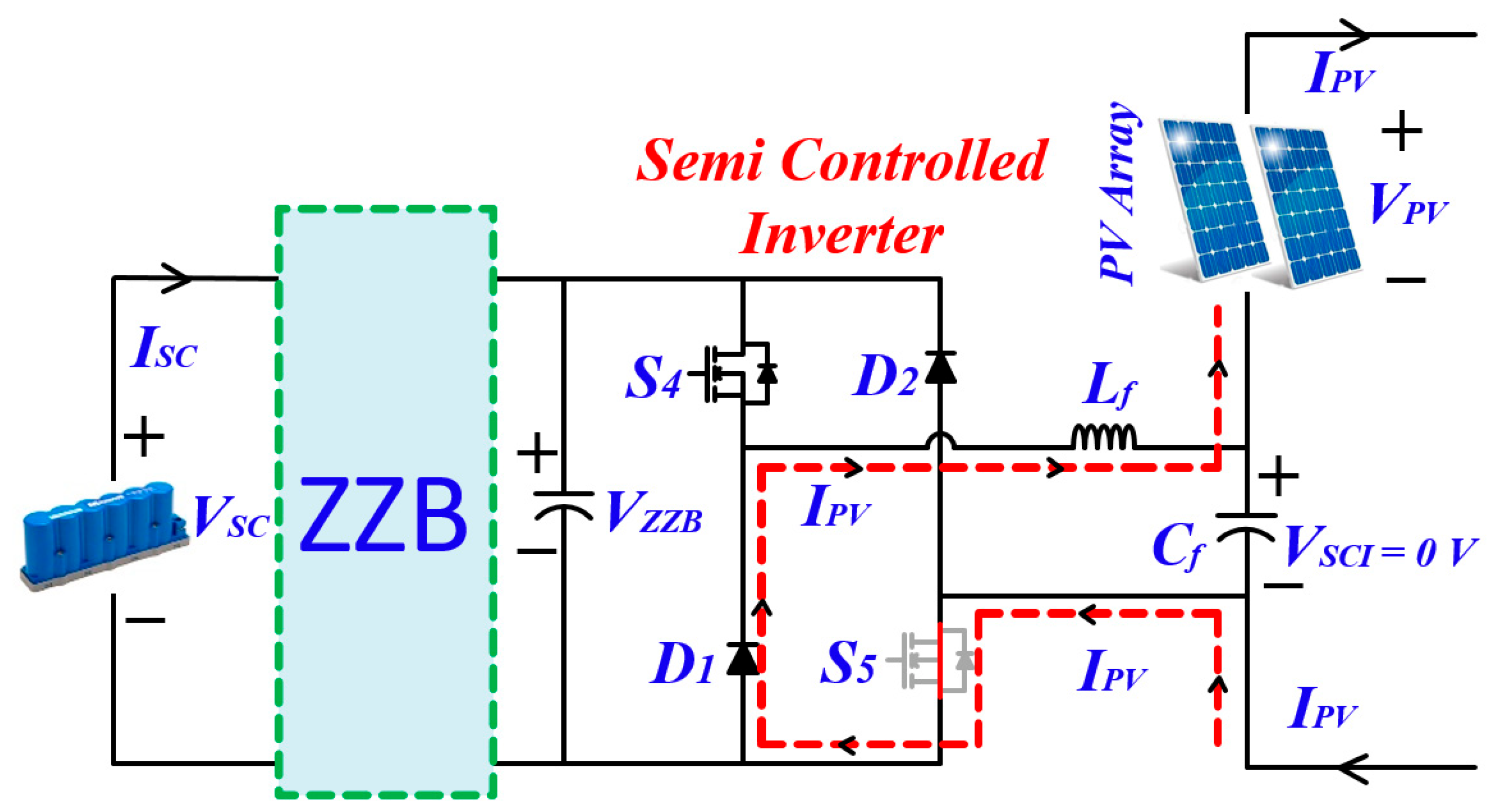
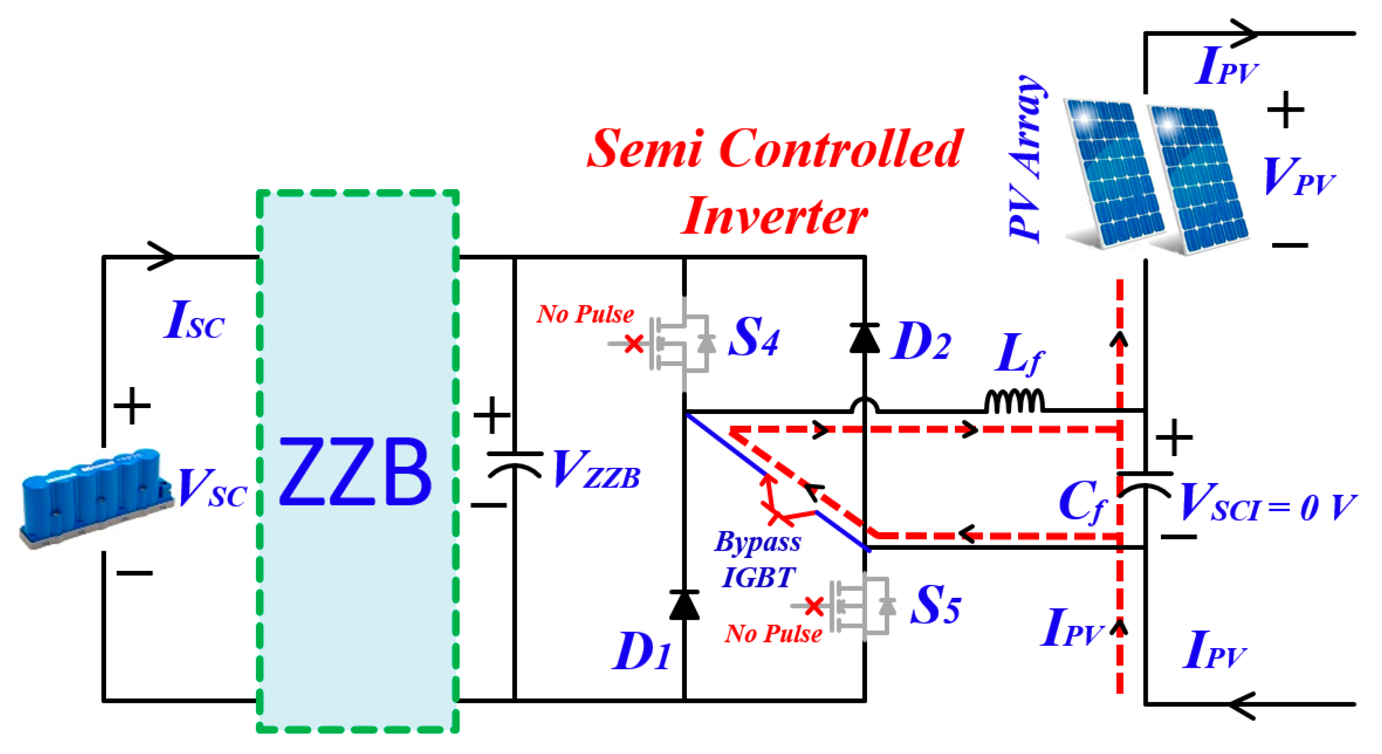
  • Secondly, the proposed topology has an inherent bypassing capability in case there is a fault in the Semi-Controlled Inverter (SCI) stage of the SC-PPS (if any of the switches are damaged/shorted due to multiple reasons). In such cases, the shorted switch will bring the output LC filter of SCI into a parallel arrangement and then into series with the PV. Thus, the DC nature the PV current will simply bypass the SC-PPS stage directly through the filter inductor of the SCI, setting the voltage output of SCI to zero, as shown in Figure 7, for cases in which only S5 is shorted. A similar response can be expected if either only S4, or both of the switches, are shorted. This inherent feature makes it superior over the conventional cascaded topologies, as there is no hindrance of the PV MPPT operation during the occurrence of faults in the SC-PPS.
• Limitations and possible solutions (if any):
  • There may be a chance of an over-voltage fault in the SC-PPS if any one switch (or both of the switches) of the SCI stops obtaining the gate pulses due to a fault in the driver circuit of the switches. This may lead to a high negative voltage continuously building at the output of both of the SC-PPSs due to the positive PV current. A proper over-voltage detection scheme can detect the fault, if one is indeed present, and the SC-PPS stage can be bypassed with a unidirectional switch (IGBT) at the input port of the LC filter of the SCI, as shown in Figure 8. This will gradually discharge the energy stored in the LC circuit and eventually bypass the SC-PPS without hampering the PV MPPT operation. Alternatively, the simplest approach may involve shutting down the entire system to rectify the fault before undertaking reinstallation. However, a more detailed analysis is indeed required to further explore the open-circuit fault-tolerant capability of the proposed system.
  • During periods in which there are no frequency events, the SCI stage always remains active (to regulate the output voltage of the SCI to zero) even though there is no active power dealt by the SC (only circulating current flow between the switches and the output LC filter of the SCI). This will lead to some additional running losses. Nonetheless, the similar bypass arrangement, as discussed in the last point, can also improve the efficiency when at an ideal level.
  • Additionally, due to the cascade connection, when the PV output will be zero and/or during night-time, it will hardly be possible to achieve frequency response services. This is the most common problem in all cascaded-type topologies; however, this may not be an issue for conventional parallel-type configurations.
• Merits over parallel-type configurations:
  Although having few limitations, the following few points make the proposed topology promising over the existing parallel-type configurations.
  • Firstly, unlike parallel-type configurations, the proposed PSCT demands simple low-gain interfacing converters for the SC stage.
  • Secondly, unlike the parallel-type configuration, the SC can be deep-discharged due to the limitation in the input voltage variation for the interfacing converter. This feature makes it superior to the parallel-type configuration as it has the potential to improve the utilization factor of the stored energy of the SC to a large extent.

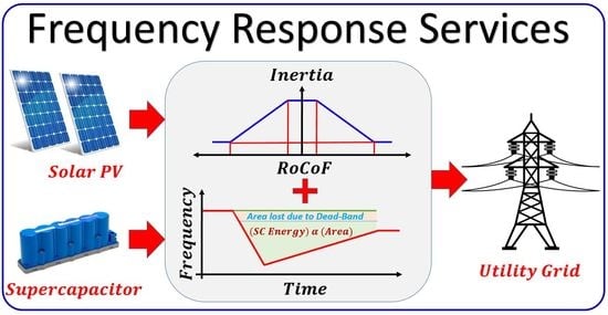
3. Frequency Response Services in PVS and the Proposed DI Dynamic Inertia Emulation

Frequency regulation is an essential part of the power system to arrest the post-disturbance frequency fluctuation within the acceptable range, and thus, to improve the resiliency of the system. In a conventional power system, frequency regulation occurs as a spontaneous response of the entire connected rotating machines post-disturbance, irrespective of their location, due to the inherent mechanical inertia. The inertia constants of the state-of-the-art rotational generators mostly fall within the range of 2 s to 6.5 s [4], which is sufficient to contain the initial post-disturbance frequency changes before the other slow-frequency control mechanisms take over the job. Meanwhile, due to inertia being a form of resistance that opposes the changes in the frequency of the system, the higher the inertia constant of the system, the better the system’s stability. Hence, this is a minimum requirement of power systems that they should poses in order to assure their resiliency. However, due to the continuous replacement of synchronous generators by power electronics converter-based DERs, which have either zero or negligible inherent inertia (the energy storing elements such as inductors and capacitors can provide small amounts of inertia), the power system experiences a rapid fall in the equivalent inertia. This concept can be well understood from Equation (1). If not taken care of beforehand, this could lead to catastrophic failures such as back-to-back blackouts. These occur due to the tripping of various relays related to load- and/or generation-shedding because of large-frequency fluctuations, higher RoCoF, deeper frequency nadirs, etc.

$$H_{eff}=\frac{{{\displaystyle \sum }}_{i=1}^m{H}_i{S}_i+{{\displaystyle \sum }}_{j=1}^n{H}_{pvj}{S}_{pvj}}{{{\displaystyle \sum }}_{i=1}^m{S}_i+{{\displaystyle \sum }}_{j=1}^n{S}_{pvj}}$$

(1)

The frequency response service that any DER should provide is basically of two types: RoCoF or Inertial Response, and Primary Frequency Response. A brief overview of both frequency response services is given below.

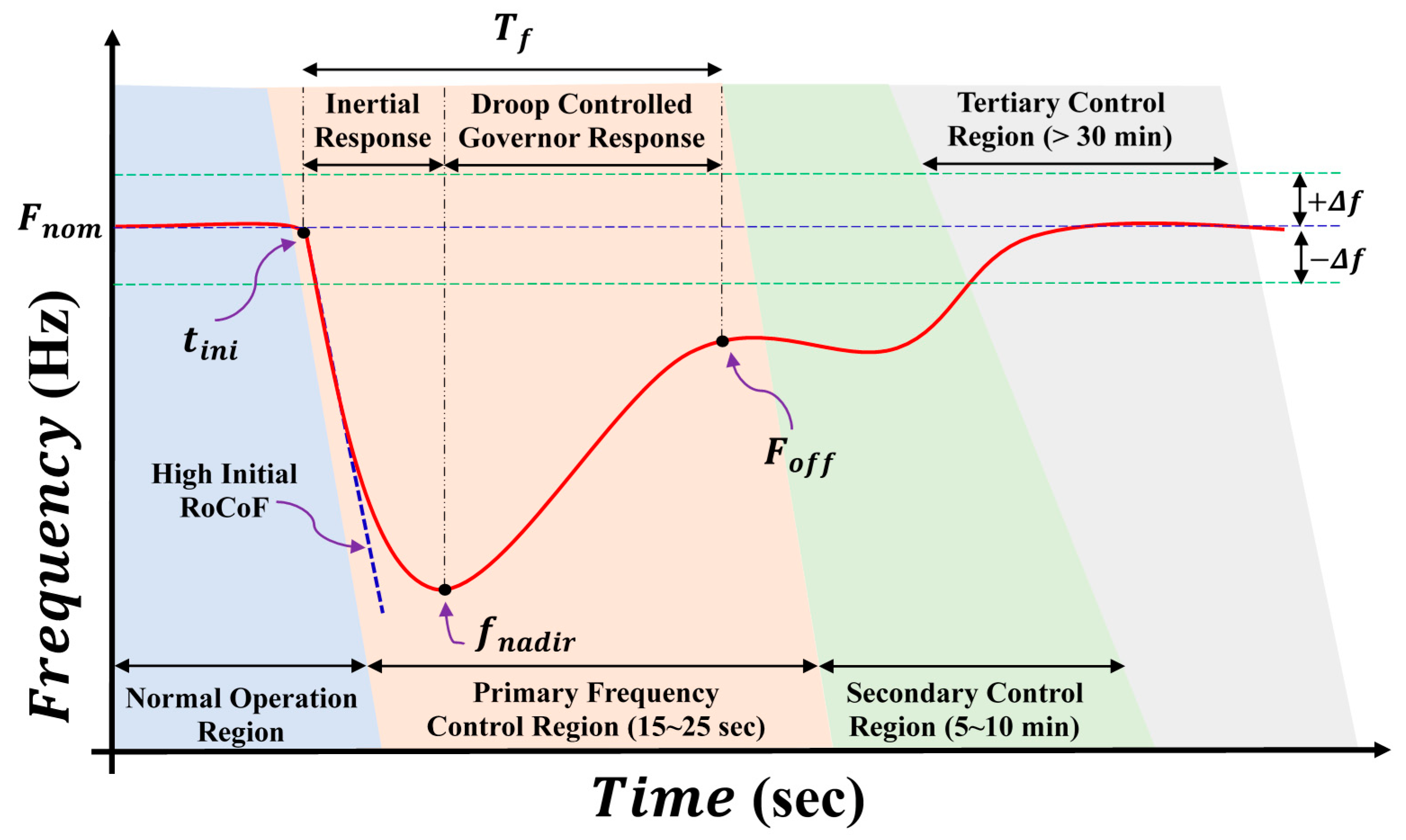
3.1. Rate of Change of Frequency (RoCoF) Response

As per the IEEE 1547-2018 standards, “Inertial response, in which the DER active power is varied in proportion to the rate of change of frequency, is not required but is permitted. If Area EPS Operator and DER Operator mutually agree to use DER inertial response, the performance requirements should be coordinated with the regional reliability coordinator with due consideration of system dynamic oscillatory behavior.” If the frequency excursion is within the continuous operating region imposed by the grid operators, the DERs should modulate their active power output as per the RoCoF scenario. This is the case provided that the averaging magnitude of the RoCoF, which corresponds to an averaging window of at least 0.1 s, is within the limit of 2.0 Hz/s for PVS, which is consistent with the specifications of Category II type DERs.

The inertia response of the DERs can be emulated based on the RoCoF and by using the swing equation, as shown below:

$$\frac{d\mathsf{\Delta }f}{dt}=\frac{\mathsf{\Delta }{P}_g-\mathsf{\Delta }{P}_d}{2H}$$

(2)

$$\mathsf{\Delta }{P}_{RoCo{F}_{pu}}=\frac{2HRoCoF}{F_{nom}}$$

(3)

where the term $\frac{d\mathsf{\Delta }f}{dt}$ indicates the RoCoF, $\mathsf{\Delta }{P}_g$ and $\mathsf{\Delta }{P}_d$ stand for the change in generation and load demand, respectively, and $H$ defines the inertia constant of the system. $\mathsf{\Delta }{P}_{RoCo{F}_{pu}}$ is the inertia response of the system in PU due to RoCoF, and $F_{nom}$ is the nominal frequency of the system. (Note: the $H$ unit is treated in “sec” if other parameters are considered in “PU”).

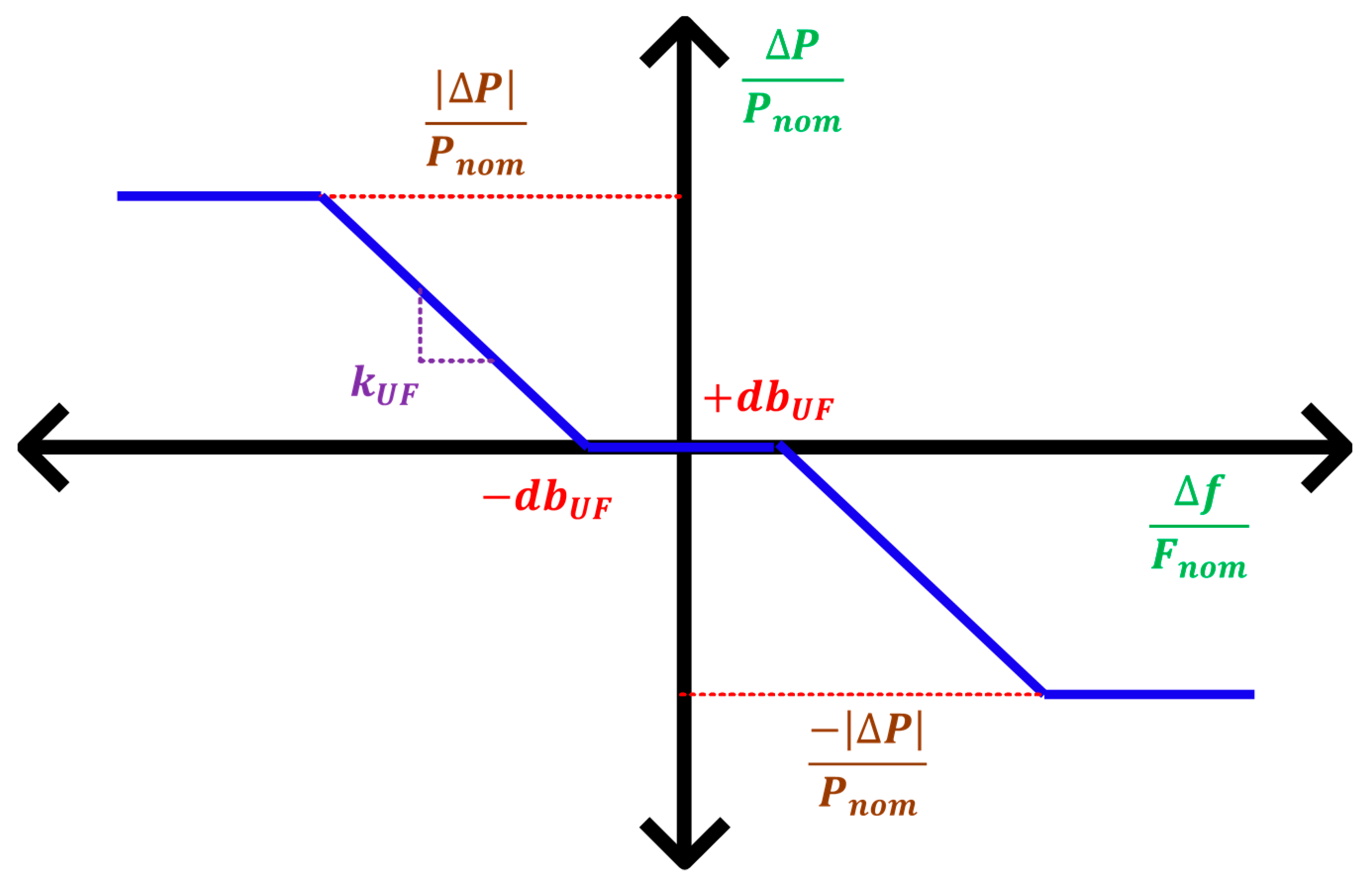
3.2. Primary Frequency Response and Frequency-Droop (Frequency-Power) Capability of the DERs

The frequency response characteristics of a typical power system mainly consist of three parts, Primary Frequency Control, Secondary Control and Tertiary Control, as shown in Figure 9. As the PFC is critical in terms of power system stability, it is the most important service. Therefore, for this paper, the topic of interest is PFC only and the SFC and TC will not be covered in detail. The PFC can further be divided into two subparts: the former inertial response and the latter governor response. In the case of conventional power systems, the initial RoCoF of the PFC characteristics, from the moment after the disturbance $\left(t_{ini}\right)$ until the point of the frequency nadir $\left(f_{nadir}\right)$, is limited by the inherent mechanical inertia of the system. However, the slow governor action comes into effect from the point of $f_{nadir}$ until the point of offset frequency $\left(F_{off}\right)$ to arrest the frequency within a certain range, denoted as $F_{nom}\pm \mathsf{\Delta }f$, which is specified by the regulator. The governor action provides the frequency support based on droop power control, which is very sluggish due to several practical constraints such as the Generation Rate Constraint (GRC), the Governor Dead Band (GDB), etc. [50].

The IEEE 1547-2018 standards demand that during the temporary frequency fluctuation, if the frequency is outside of the adjustable deadband as per the standard, the DERs should modulate their active power output against the cause. In addition to the inertial response to the RoCoF, until (and unless) the frequency returns to within the specified deadband limits, the active power output should be regulated as per Equation (4), based on the typical Droop Control (DC) method, which is shown in Figure 10.

$$P_{pu}=\underset{f<F_{nom}-d{b}_{UF}}{\min }\left\{P_{pre}+\frac{\left(F_{nom}-d{b}_{UF}\right)-f}{F_{nom}\ast k_{UF}}+\mathsf{\Delta }{P}_{RoCo{F}_{pu}};P_{avl}\right\}$$

(4)

where:

• $P_{pu}$ is the total active power output in the PU of the DER nameplate active power rating during the PFR event.
• $P_{pre}$ is the pre-disturbance power of the DER in the PU at the moment after the frequency crosses the dead band.
• $P_{avl}$ is available active power in the PU of the DER rating.
• $f$ is the instantaneous system frequency.
• $d{b}_{UF}$ corresponds to dead band of the droop control, and $k_{UF}$ stands for the droop coefficient under-frequency events.

Similarly, the total absolute active power, which should be dealt by the DERs during PFR $\left(\mathsf{\Delta }{P}_{PFR}\right)$, can be written as:

$$\mathsf{\Delta }{P}_{PFR}=\mathsf{\Delta }{P}_{Droop}+\mathsf{\Delta }{P}_{RoCoF}=\frac{P_{nom}}{F_{nom}}\left[{\left\{\frac{\left(F_{nom}-d{b}_{UF}\right)-f}{k_{UF}}\right\}}_{f<F_{nom}-d{b}_{UF}}+2HRoCoF\right]$$

(5)

where $P_{nom}$ is the nominal power rating of the system and $\mathsf{\Delta }{P}_{Droop}$ and $\mathsf{\Delta }{P}_{RoCoF}$ are the absolute power contribution towards PFR considering the droop response and RoCoF response respectively.

The power mismatch in case of over-frequency PFR can be taken care of without additional energy storage just by curtailing the PV power generation by operating in the MPPT region. Thus, in this paper, the PFR of the PV-based DERs will be discussed only for the under-frequency phenomenon, which mostly happens because of a sudden increase in load demand.

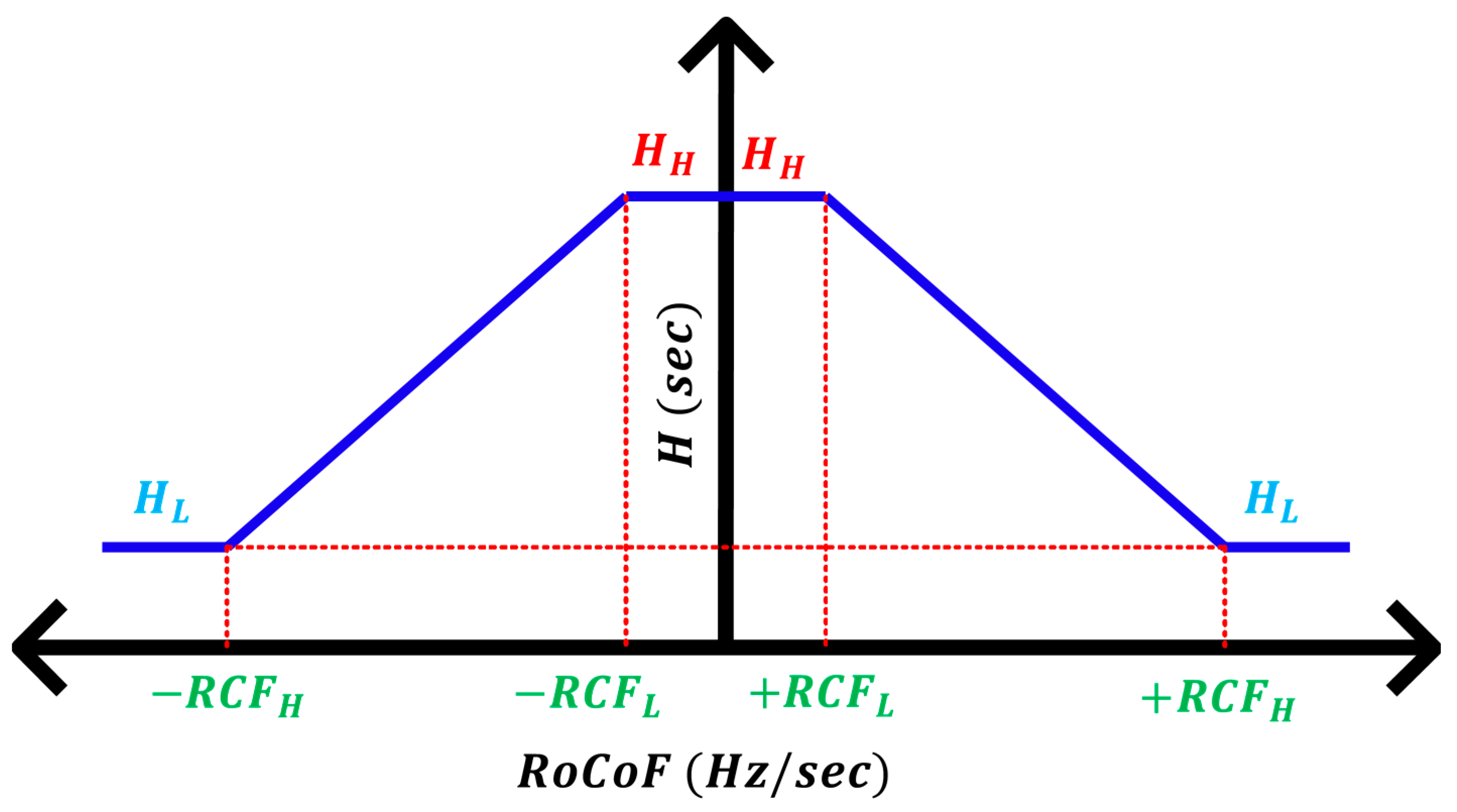
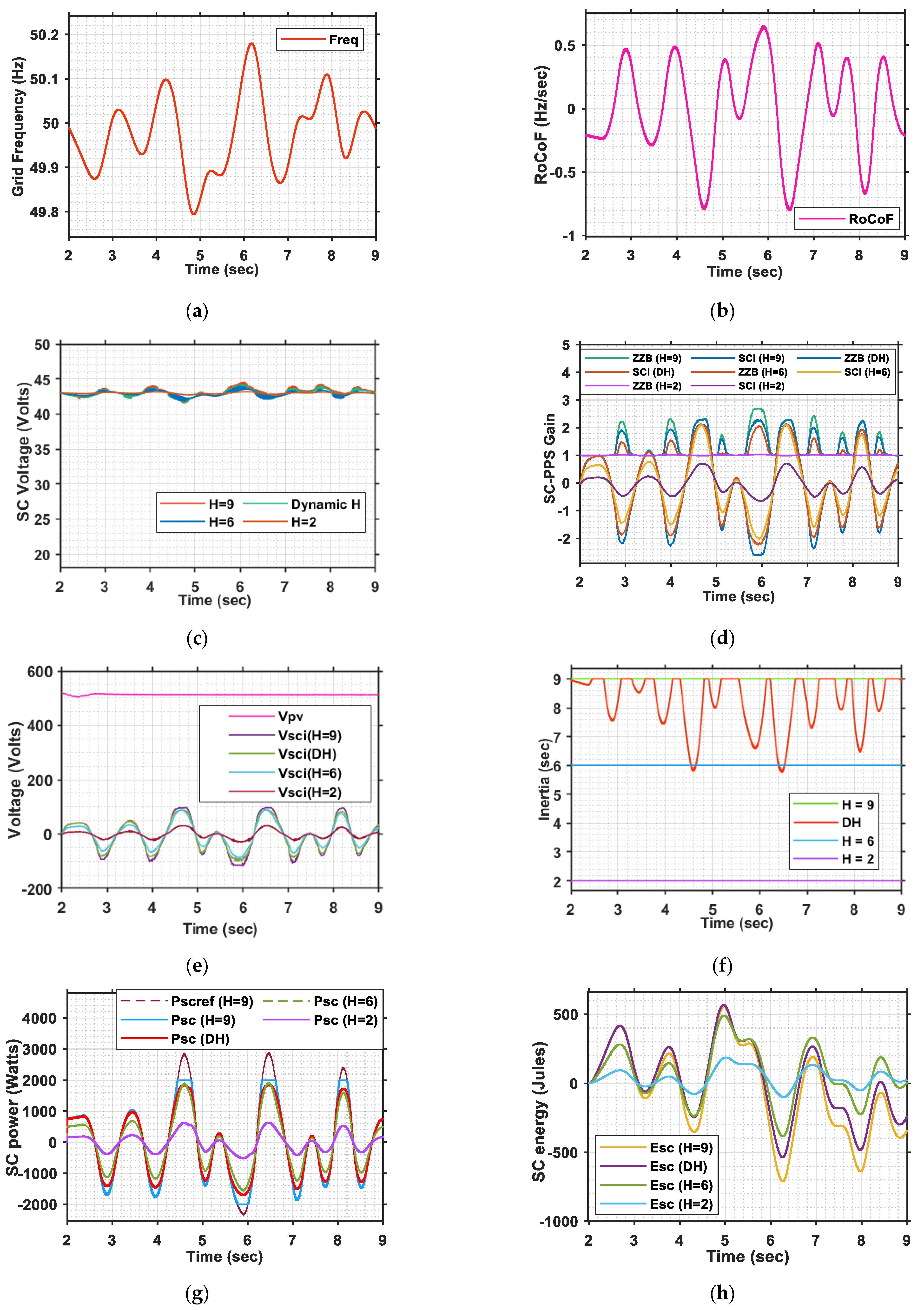
3.3. Proposed Dynamic Inertia Emulation Based on Droop-Inspired Method for PVS

As indicated in Equation (3) of the previous sub section, the inertia response of the DERs for a specific RoCoF can be emulated using the concept of swing equation-like conventional generators. Therefore, if correlated with the power electronics-based DERs such as the PV-SC system, the same differential power should come from the SC and can be rewritten as:

$$P_{S{C}_{RoCoF}}=\mathsf{\Delta }{P}_{RoCo{F}_{pu}}{P}_{nom}=\frac{2H{P}_{nom}RoCoF}{F_{nom}}$$

(6)

where $P_{S{C}_{RoCoF}}$ is the absolute value of the power dealt by the SC storage unit.

In the case of the classical power system, the inertia constant offered by the state-of-the-art rotating machines is never a fixed value, but rather, a variable one. It strictly depends on its type, whether it is a thermal generator, tidal power generator or hydropower generating unit. The capacity of the plant is also major factor to decide the $H$ value of that particular generating unit. Therefore, it is very crucial to select an appropriate value of $H$ for the PVS such that it will behave in a similar or better way compared its classical counterparts while arresting the frequency disturbances. Moreover, as, there are no such standards imposed by the national and/or international grid codes, which specify the values of $H$ that the DERs should emulate, the flexibility in the hands of the designer to select the parameters freely, but this flexibility is constrained by the power- and energy-handling capability of the available/targeted storage.

Here, the authors proposed a novel Droop-Inspired (DI) method, which assumes a range of values for the inertia constant ($H_L$ to $H_H$) to emulate dynamic inertia ($H_D$) for the PVS as a function of RoCoF, and thus, to utilize the available storage in a better way. The aim was to achieve better inertia response during low-RoCoF periods ($\left|RoCoF\right|<RC{F}_L$) by subjecting the system to higher $H$ values ($H_D$ = $H_H$), where $H_H$ should be higher than the maximum inertia offered by any alternators in scale. This will help to achieve a better grip in terms of arresting the frequency disturbance in a faster way at the root level itself in order to avoid the very real possibility of larger-scale future catastrophes. However, during comparatively higher RoCoF, the same cannot be expected due to the limitation in the available power and/or energy from the storage unit. So, during medium level RoCoF ($RC{F}_L\le \left|RoCoF\right|<RC{F}_H$), the system can be subjected to variable $H$ values ($H_H>H_D>H_L$) as a linear function of RoCoF. Similarly, during high level RoCoF ($\left|RoCoF\right|\ge RC{F}_H$), the system can be subjected to lower $H$ values ($H_D$ = $H_L$) (but not lower than the lowest inertia type synchronous generators in terms of scale) to avoid unnecessary increases in the power and energy rating of the SC. Mathematically, $H_D$ can be expressed as:

$$H_D=\left\{\begin{array}{ll}\hfill H_H,& \left|RoCoF\right|<RC{F}_L\hfill \\ \hfill \left(\frac{H_L-H_H}{RC{F}_H-RC{F}_L}\right)\left(\left|RoCoF\right|-RC{F}_L\right)+H_H,& RC{F}_L\le \left|RoCoF\right|\le RC{F}_H\\ \hfill H_L,& \left|RoCoF\right|>RC{F}_H\end{array}\right.$$

(7)

The proposed DI method is shown in Figure 11, where $H_H$ and $H_H$ are high and low values of the inertia constant set by the designer and $RC{F}_H$ and $RC{F}_L$ are the high and low values of the RoCoF that the system should take care of.

The advantages of the proposed dynamic inertia, based on the DI method, as compared to fixed inertia are better justified through the following points:

1.

The conventional constant inertia-based approach (a narrow range of RoCoF will be serviced):

In standard practice, the storage is mostly sized based on the worst case RoCoF the system is designed to target, and is subject to the virtual inertia constant the designer has set for the system. Therefore, in the case of constant inertia emulation methods:

• During low-RoCoF periods, the reference power and energy demanded by the control are proportionately less and, hence, are dealt by the storage. This underutilizes the storage although it is capable enough of dealing with more power and energy. Thus, smaller disturbances may lead to larger frequency fluctuation, making the system less robust.
• On the contrary, during high-RoCoF periods, the maximum RoCoF that can be addressed is also limited to the storage capability as the corresponding power and energy demands are high for the same inertia constant.

The above two issues motivated the authors to come up with the concept of the adjustable inertia.

2.

The proposed adjustable inertia-based approach (capable of addressing a wider range of RoCoF values with limited storage capability compared to its conventional counterparts):

• During low-RoCoF periods, the proposed method helps in emulating comparatively larger inertia than that of the Synchronous Machines in terms of scale (such as: thermal generators, pumped storage types, open cycle gas turbines, etc. [4]). Thus, it utilizes the storage capability to a large extent, allowing the storage to deal with more power and energy fluctuation (but within the limits of its capability). This will help in curbing the frequency fluctuation at the root level itself. Thus, an extreme frequency fluctuation and, in turn, an anticipated grid failure can be avoided.
• However, we cannot expect similar performance (larger inertia emulation) during high-RoCoF periods as it will ultimately demand larger storage size. Thus, the control is designed in such a way that it ensures minimum inertia (not less than that of the class of synchronous generators with the lowest inertia-emulating capabilities such as: hydro turbines and combined cycle-type generating stations etc. [4]).

Thus, the proposed approach justifies its superiority over the classical constant inertia-based approaches in terms of both making the grid frequency more stable and utilizing a smaller storage space for a wider range of RoCoF values ($\le \pm RC{F}_H \mathrm{Hz}/\mathrm{s}$), with an adjustable inertia varying from ($H_L$ to $H_H$) s in PU.

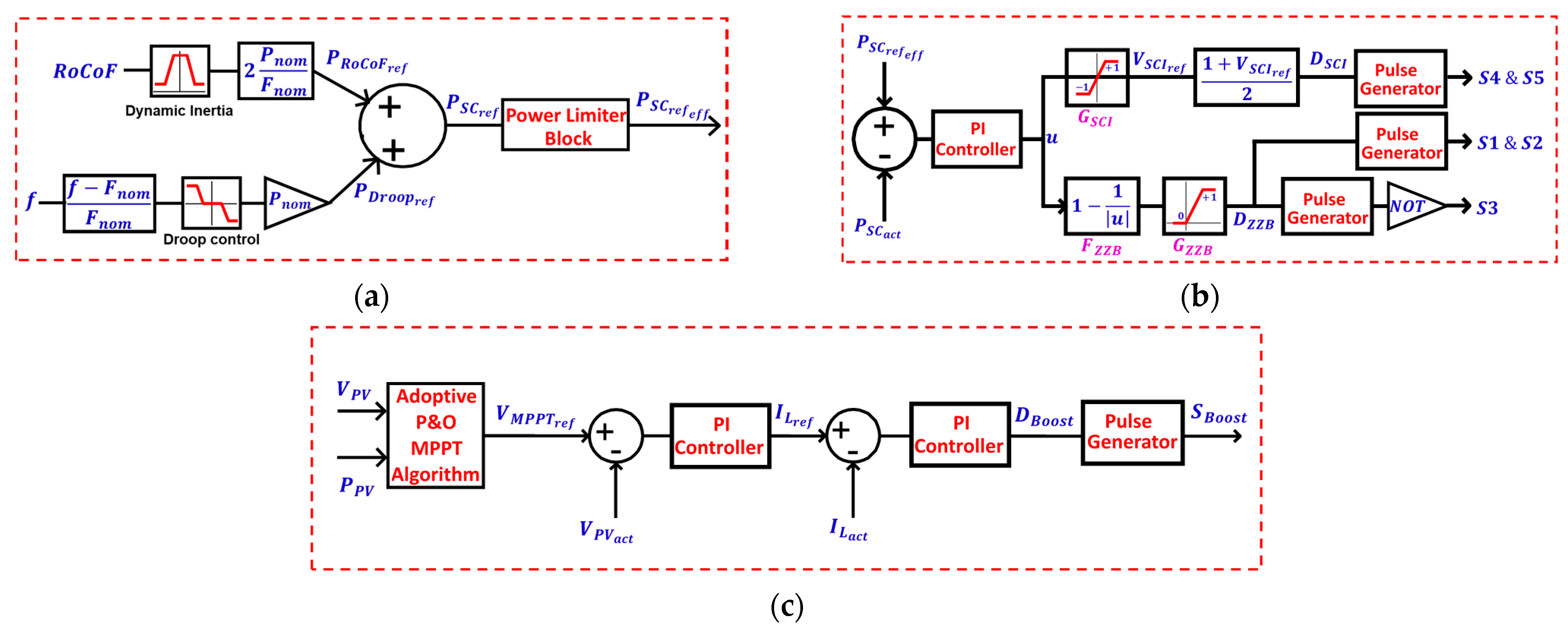
4. Implemented Control Schemes

This section gives a clear-cut idea about the various implemented control schemes for the different PPS of the proposed PSCT. It is divided into three major parts:

• The proposed charge control scheme for SC using ZZB and SCI.
• MPPT control for the PV using the Boost Converter.
• DC-link voltage control and grid side control using a three-phase two-level VSI.

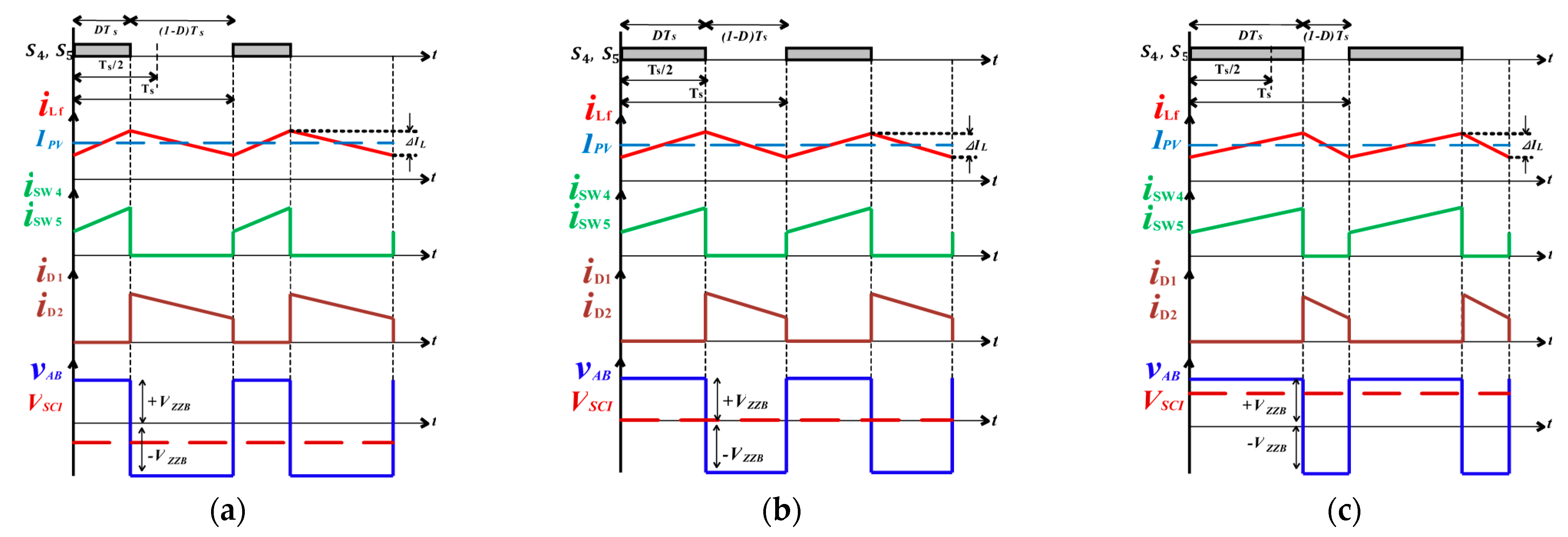
4.1. Charge Control Scheme for SC Using ZZB and SCI

The implemented charge control scheme for the SC consists of two parts, the outer loop for the generation of reference power for the SC based on the frequency profile, and the inner loop to decouple the operation of ZZB from that of SCI and to produce appropriate duty levels for both converters.

4.1.1. The Outer Control Loop for the Reference Power Generation

In the case of conventional control methods, the PFR is generally addressed only through the Droop control method, which fails to address the high initial RoCoF due to the incorporated deadband in the Droop control. However, as per the IEEE 1547-2018 edition, the Category II-type Distributed Generators (Mostly Solar PV) should adjust their output based on the Droop control method in addition to the Synthetic inertia response based on RoCoF. The proposed combined control method is capable of addressing this point in a more straightforward way via the outer control loop for the SC-PPS, as shown in Figure 12a. It is a combined control platform for both SIR as well as PFR, where the reference power for SIR $\left(P_{SI{R}_{ref}}\right)$ and the reference power for PFR $\left(P_{PF{R}_{ref}}\right)$ can be estimated using the proposed DI-based dynamic inertia emulation method and the conventional droop control method. This means the single control method (Droop Control + RoCoF response) can emulate both the mechanical inertia of the rotor (Instant Reflex) as well as the governor response (Slow Response). Algebraically, the total calculated reference power for SC $\left(P_{S{C}_{ref}}\right)$ is the union of both $P_{SI{R}_{ref}}$ and $P_{PF{R}_{ref}}$, as expressed in Equation (8). This means that during low-frequency fluctuations (within $\pm d{b}_{UF}$ set by the designer), only the RoCoF response will be active, whereas, during comparatively larger under-frequency events (for frequency fluctuations of less than $-d{b}_{UF}$), the droop response part will also come into action, including the RoCoF response. Finally, the effective reference power for SC $P_{S{C}_{re{f}_{eff}}}$ is decided by a power limiter block, as expressed in Equation (9), which places a limit on the calculated $P_{S{C}_{ref}}$. This ensures that the SC-PPS is not overloaded and the SC is not charged or discharged beyond its upper or lower voltage limits.

$$P_{S{C}_{ref}}=P_{SI{R}_{ref}}\cup P_{PF{R}_{ref}}=\left\{\begin{array}{cc}\hfill \frac{2H{P}_{nom}RoCoF}{F_{nom}},& if f>F_{nom}-d{b}_{UF}\\ \hfill \frac{P_{nom}}{F_{nom}}\left\{\frac{\left(F_{nom}-d{b}_{UF}\right)-f}{k_{UF}}+2HRoCoF\right\},& if f<F_{nom}-d{b}_{UF}\end{array}\right.$$

(8)

$$P_{S{C}_{re{f}_{eff}}}=\left\{\begin{array}{cc}\hfill max\left(min\left(P_{S{C}_{ref}},+P_{S{C}_{nom}}\right), 0\right),& if V_{SC}\ge V_{S{C}_{max}}\hfill \\ \hfill max\left(min\left(P_{S{C}_{ref}},+P_{S{C}_{nom}}\right),-P_{S{C}_{nom}}\right),& if V_{S{C}_{min}}<V_{SC}<V_{S{C}_{max}}\hfill \\ \hfill min\left(max\left(P_{S{C}_{ref}},-P_{S{C}_{nom}}\right), 0\right),& if V_{SC}\le V_{S{C}_{min}}\hfill \end{array}\right.$$

(9)

where $P_{S{C}_{nom}}$ is the nominal power rating of the SC-PPS. $V_{S{C}_{max}}$ and $V_{S{C}_{min}}$ are the upper and lower voltage limits of the SC, respectively. All these limits are decided in the sizing section of this paper.

4.1.2. The Inner Control Loop to Decouple the ZZB Operation from SCI

As mentioned before, there are two stages for the power processing of the SC. The first stage involves the use of a ZZB-based DC–DC converter to provide the required voltage gain, and the second stage involves the use of a semi-controlled inverter or a polarity changer, which decides the appropriate polarity of the series-injected voltage with the PV to carry out either charging or discharging operation of the SC. However, proper decoupling of the control of both power stages is highly essential. Here, the authors proposed a single PI-controller-based decoupling method to decouple the ZZB operation from the SCI operation. The block diagram of the proposed decoupled control is shown in Figure 12b. The common PI controller block takes the error between the $P_{S{C}_{re{f}_{eff}}}$ and the actual power of the SC $\left(P_{S{C}_{act}}\right)$ as inputs and produces the reference duty for the ZZB $\left(D_{ZZB}\right)$ and the PU reference voltage for the SCI $\left(V_{SC{I}_{ref}}\right)$ with the help of a few function blocks and saturation blocks. The logic behind this control is not to change the duty of both the ZZB and SCI simultaneously. Rather, the SCI will come into picture to regulate the magnitude and polarity of its output voltage only when ZZB is bypassed or operated at a gain level of unity by saturating the $D_{ZZB}$ to zero with the help of the saturation block $\left(G_{ZZB}\right)$. On the contrary, the function block $\left(F_{ZZB}\right)$ after the PI controller will decide the appropriate $D_{ZZB}$ to boost the voltage only when the PI controller output $\left(u\right)$ falls in the range of $\left(\left|u\right| >1\right)$. During that moment, the $V_{SC{I}_{ref}}$ is either saturated to +1 or −1 with the help of a saturation block $\left(G_{SCI}\right)$ connected at the output of $u$. The second function block $\left(F_{SCI}\right)$ takes the $V_{SC{I}_{ref}}$ as input and produces the appropriate duty $\left(D_{SCI}\right)$ for the SCI.

4.2. Implemented MPPT Control for the Boost Converter

A two-level control scheme is implemented here using an adaptive P&O algorithm for the MPPT operation of the PV, as shown in Figure 12c. The outer voltage loop takes the error between the reference MPPT voltage $\left(V_{MPP{T}_{ref}}\right)$, generated by the adaptive P&O, and the actual PV voltage $\left(V_{P{V}_{act}}\right)$ as inputs and produces the reference current $\left(I_{L_{ref}}\right)$ for the inner current control loop. Finally, the PI controller of the inner current control loop will produce the appropriate duty for the Boost converter $\left(D_{Boost}\right)$, which will allow the MPPT operation to happen. The advantage of the adaptive P&O algorithm over the classical P&O and IC algorithm is that it can minimize the power oscillation problem across the MPP point to a large extent. This can be achieved by conducting dynamic step changes in the reference voltage as a function of the changes in the actual PV power $\left(\mathsf{\Delta }{P}_{P{V}_{act}}\right)$ instead of a constant step change for each time the algorithm is executed. This will help $V_{MPP{T}_{ref}}$ to settle at the MPP more quickly as well as to avoid hovering around the MPP point. As a result, not only will the MPPT tracking efficiency be improved, but the DC-link voltage ripple will also be less for similar DC Link capacitance values, resulting in less interference in the inverter side control. Mathematically, the expression for the dynamic step change in $V_{MPP{T}_{ref}}$ can be as expressed as in Equation (10).

$$\mathsf{\Delta }{V}_{MPP{T}_{ref}}=k\left\{P_{P{V}_{act}}\left(i\right)-P_{P{V}_{act}}\left(i-1\right)\right\}$$

(10)

where k is a constant, which is a design constraint that is specific to the dynamics of the MPPT tracking speed and/or the dynamics of the converter.

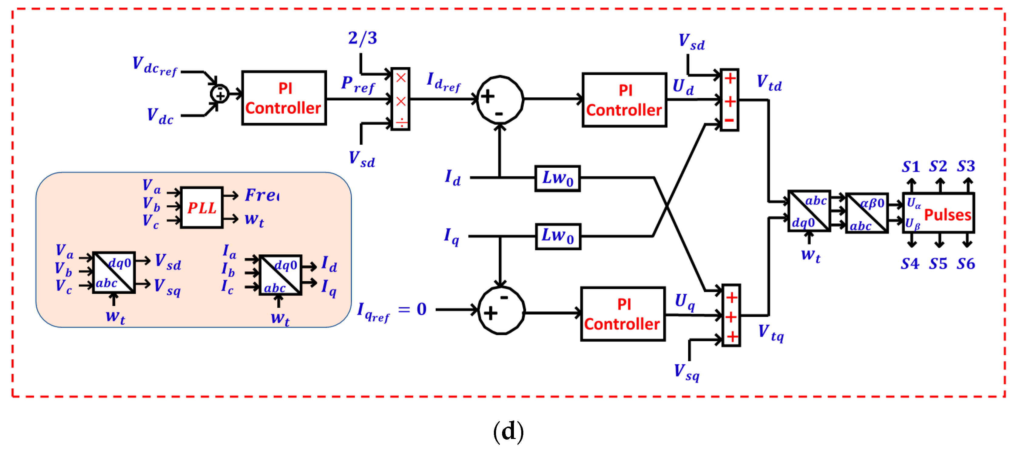
4.3. DC Link Voltage and Grid Side PQ Control Scheme Using a Three-Phase Two-Level VSI

The classical two-level control method is implemented here for the inverter based on the $dq$ reference frame to achieve decoupled control over the active and reactive power sources that are fed to the grid. The PLL ensures the synchronism process by setting the $q$ axis component of the grid voltage to zero, such that the $d$ axis component of the grid voltage can be aligned to the zero axis of the $abc$ frame of reference; thus, it provides the required phase shift to the rest of the control loop. The block diagram of the implemented control is shown in Figure 12d. As we can see, the outer voltage control loop provides the reference power and, in turn, the reference $d$ axis component of the inverter output current to the inner current loop control. Similarly, the reference $q$ axis component of the inner current control loop is set to zero to ensure unity power factor at the PCC. The $d$ and $q$ axis components of the PCC voltage, and the drop in the filter inductors that occurs due to $d$ and $q$ axis components of the inverter output current, are directly connected, as feed-forward terms, to the inner current control loops. This, these are then taken forward to produce the reference three-phase rotating voltages with the help of the Park transformation and, in turn, the PWM pulses for the inverter.

The control gain parameters for the different power-processing stages of the proposed topology are mentioned in

Table 2. Control gain parameters for the different power-processing stages of the proposed PSCT.

Power-Processing Stages	Control Gain
Zig-Zag Boost and Semi-Controlled Inverter	Kp = 0.1 and Ki = 40
Boost Converter for PV MPPT	Outer Voltage Loop: Kp = 200 and Ki = 1000 Inner Current Loop: Kp = 0.001 and Ki = 20
3 Phase Inverter for DC-link voltage control	Outer Voltage Loop: Kp = 10 and Ki = 100 Inner Current Control Loop: Kp = 1 and Ki = 50

.

5. Methodology for Sizing of the SC Storage System

This section discusses the proposed methodology for the sizing of SC storage system to address the targeted frequency response services. The sizing of SC storage system can also be described as the fixing of energy requirement of the SC modules and power rating of the associated power stages. The fixing of the power rating of the SC module is not a major concern, as it can ideally handle any amount of burst power; however, in practical terms, the peak power rating of the SC can be as high as 10 times its nominal power rating. Below are several considerations to be noted before undertaking the sizing of the SC storage system:

• The synthetic energy response is a high-power intensive service; however, the average energy demand, at the scale of a few seconds, is almost zero due to the frequent zero crossing of the RoCoF (zero net energy impact).
• The primary frequency response is intense not only in terms of power but also in terms of energy demand due to its comparatively longer event duration.
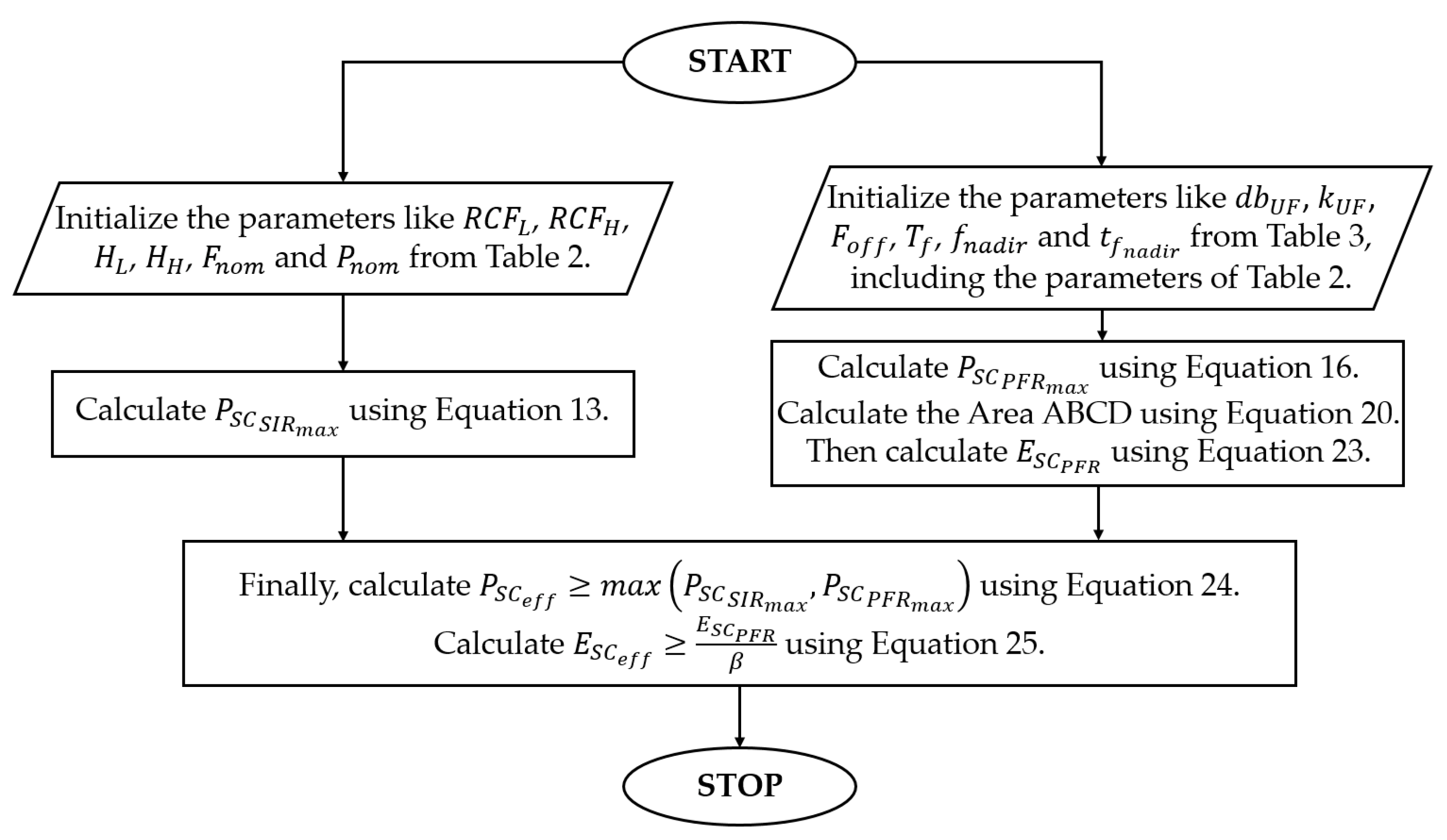
• Therefore, the power rating estimation of the SC-PPS ($P_{S{C}_{max}}$) should be decided by considering both the SIR and the PFR.
• However, the energy rating of the SC modules ($E_{SC}$) should be decided based only on the PFR.

5.1. Methodology Based on the Synthetic Inertia Response or the RoCoF Response

In this subsection, the power estimation of the SC-PPS is carried out considering the proposed DI method for dynamic inertia emulation. The peak power demand of the SC-PPS is estimated for the system under consideration in Section 2 and the set of design parameters considered in

Table 3. Design parameters for DI-based Dynamic Inertia emulation method.

Design Parameters	Ratings
$P_{nom}$	10 kWp
$F_{nom}$	50 Hz
Maximum allowable frequency fluctuation in PU with respect to $F_{nom}$	$\pm 0.03$ PU
Time constant of the averaging window for RoCoF	20 ms
$RC{F}_L$1	$\pm$0.2 Hz/s
$RC{F}_H$1	$\pm$1.5 Hz/s
$H_L$2	2 s
$H_H$2	9 s

¹ The setting of these values is in the hands of the designer, subject to availability or the targeted storage and the targeted range of RoCoF to be served. ² The inherent inertia value offered by the classical rotating machines mostly falls in the range of 2 to 6 s. Therefore, the $H_L$ and $H_H$ values are chosen accordingly to obtain similar or better responses, but it is still a design constraint.

. Here, it was assumed that a 10 kWp PV system was connected to a small isolated network of an island that had high levels of with wind generation during the day time, and which experienced rapid wind variation, resulting in intense frequency fluctuations.

Now, using the Equations (6) and (7), if we plot the instantaneous power of the SC vs. the RoCoF using the set of parameters in Table 3, they will follow a kind of parabolic characteristics, as shown in Figure 13. From Figure 13, it can be seen that the absolute peak SC power demanded by the system appears in the droop region of the characteristics and is almost 1.9 kW at an absolute RoCoF value of nearly 0.9 Hz/s. Here, a generalized mathematical approach was also carried out by the authors to derive the expression of $P_{S{C}_{max}}$ with the knowledge of only such parameters as $RC{F}_L$, $RC{F}_H$, $H_L$, $H_H$, $F_{nom}$ and $P_{nom}$, as derived below.

From Equations (6) and (7), the instantaneous SC power expression PSC for the droop region of the characteristics can be written as:

$$P_{SC}=\frac{-2P_{nom}RoCoF}{F_{nom}}\left\{\left(\frac{H_L-H_H}{RC{F}_H-RC{F}_L}\right)\left(\left|RoCoF\right|-RC{F}_L\right)+H_H\right\}$$

(11)

Now, differentiating the above expression with respect to RoCoF and then equating to zero, we obtain the expression for the absolute value of RoCoF at which the maximum SC power $\left(P_{S{C}_{max}}\right)$ occurred, as stated in Equation (12):

$${\left|RoCoF\right|}_{P_{S{C}_{max}}}=\frac{RC{F}_L\left(H_L-H_H\right)-H_H\left(RC{F}_H-RC{F}_L\right)}{2\left(H_L-H_H\right)}$$

(12)

Substituting Equation (12) in Equation (11), we obtain the final expression for the maximum SC power for SIR $\left(P_{S{C}_{SI{R}_{max}}}\right)$, as stated in Equation (13):

$$\left|P_{S{C}_{SI{R}_{max}}}\right|=\left|\frac{{\left[RC{F}_L{H}_L-RC{F}_H{H}_H\right]}^2{P}_{nom}}{2\left(H_L-H_H\right)\left(RC{F}_H-RC{F}_L\right)F_{nom}}\right|$$

(13)

where $+RoCo{F}_{P_{S{C}_{max}}}$ leads to $-P_{S{C}_{SI{R}_{max}}}$, i.e., the estimated maximum charging power requirement of the SC-PPS; conversely, $-RoCo{F}_{P_{S{C}_{max}}}$ leads to $+P_{S{C}_{SI{R}_{max}}}$, i.e., the estimated maximum discharging power requirement of the SC-PPS.

An example case is solved below using the given set of parameters in Table 3 for a given low-frequency fluctuation profile as an input to the system, and the corresponding MATLAB simulation results are also shown in Figure 14 to justify the estimation method.

Example 1.

Inputting the parameter values of Table 3 into Equation (13), we can calculate the power rating of SC-PPS as below.

$$\left|P_{S{C}_{SI{R}_{max}}}\right|=\left|\frac{{\left[0.2\times 2-1.5\times 9\right]}^2\times \mathrm{10,000}}{2\left(2-9\right)\left(1.5-0.2\right)\times 50}\right|=1885 \mathrm{Watts}$$

The calculated $P_{S{C}_{SI{R}_{max}}}$ exactly matches the graphically estimated data of Figure 13. Additionally, from Figure 14, it is observed that, for the targeted range of low-frequency fluctuations, a RoCoF as high as $\pm$1.1 Hz/s can be easily serviced with the storage capacity of 2 kW and almost zero net energy requirement over a period of few seconds. This is mostly due to the emulation of the dynamic inertia constant by the PVS.

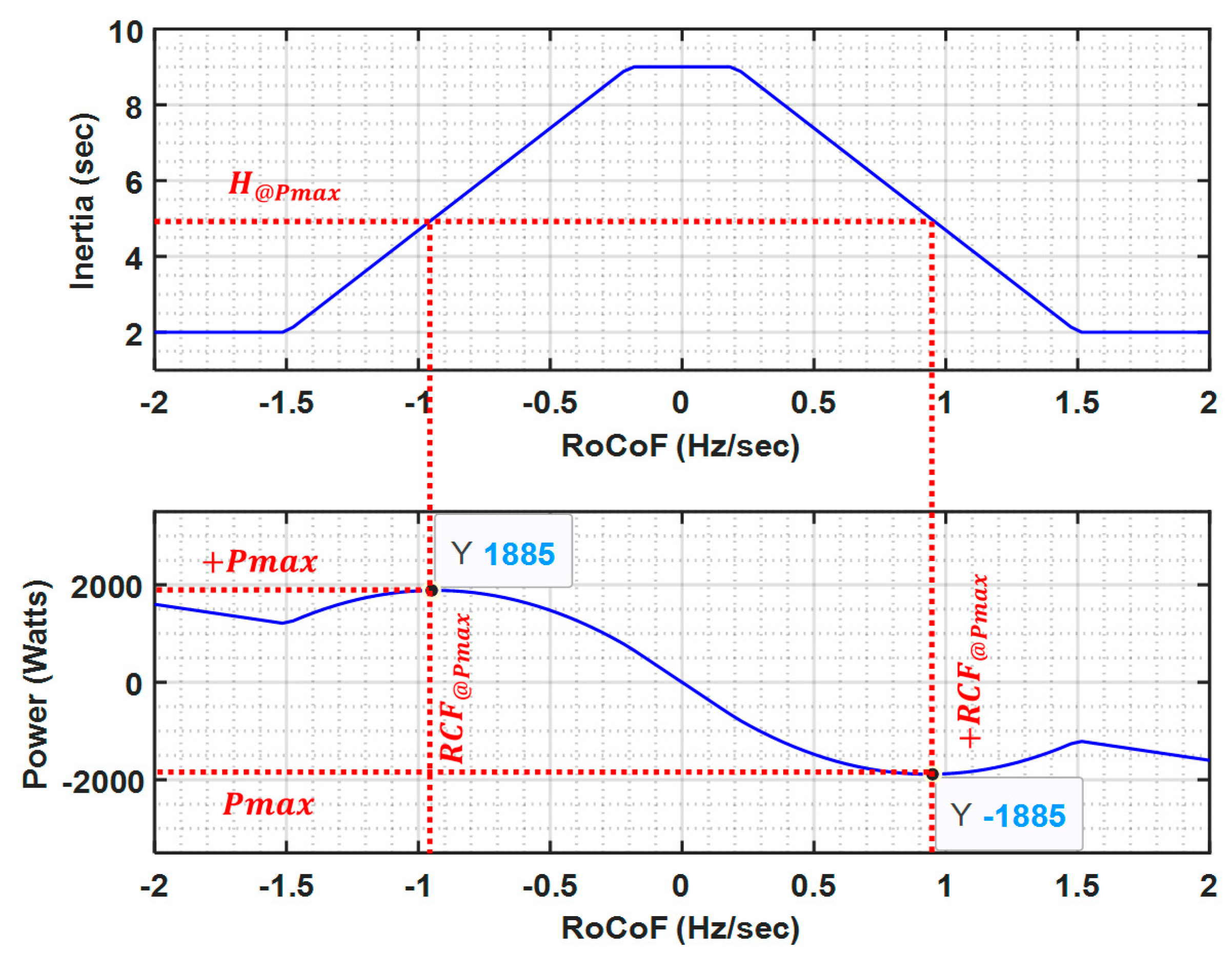
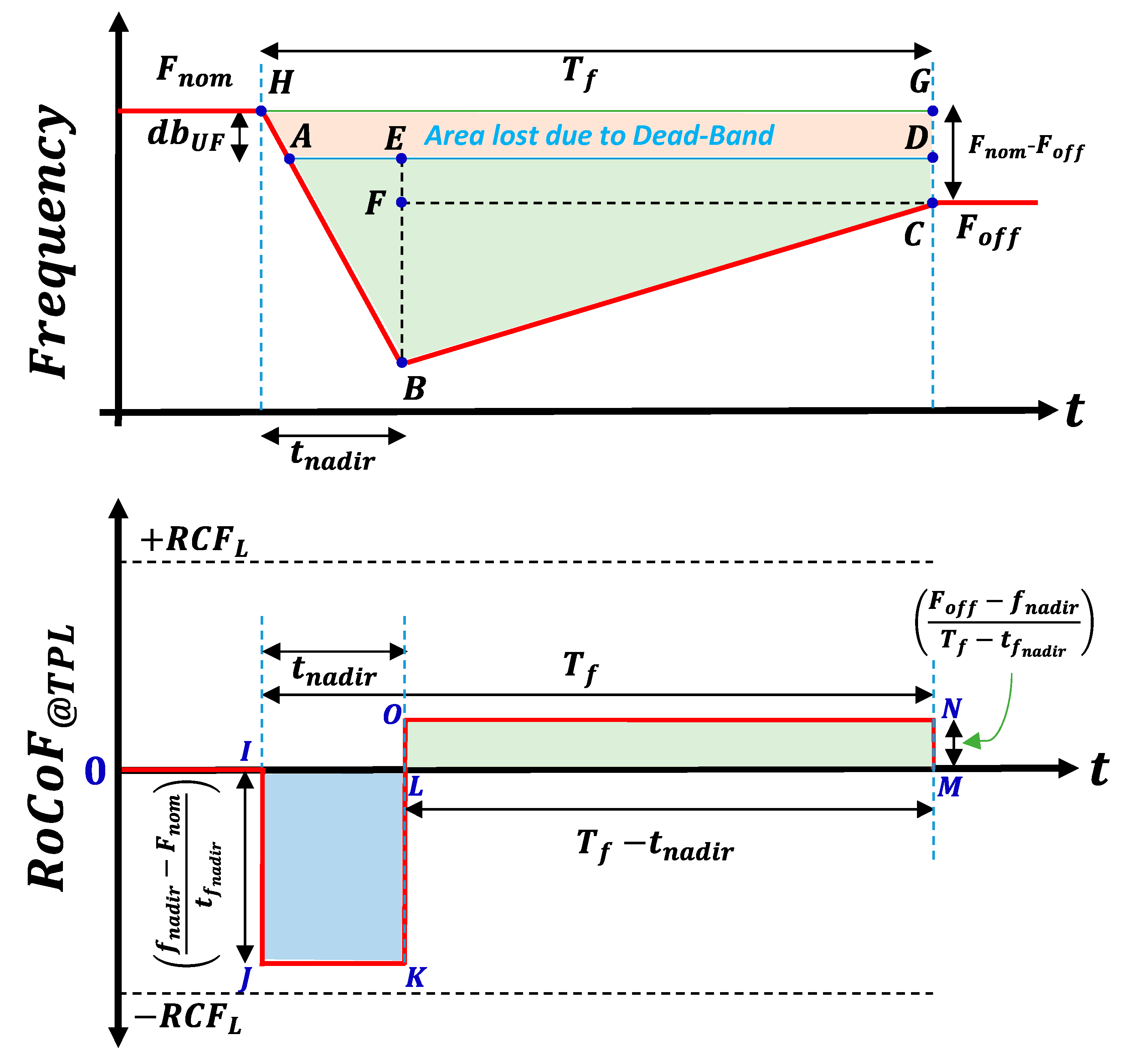
5.2. Methodology Based on the Primary Frequency Response

For the estimation of power and energy demand by the under-frequency events, it is very important to obtain the information on the containment period frequency profile. Usually, the envelope of the under-frequency event is not unique. Moreover, the severity of the event may differ in terms of either the duration of the containment zone ($T_f$), the depth of the event ($f_{nadir}$), the occurrence of $f_{nadir}$ with respect to $T_f$ ($t_{f_{nadir}}$) the final offset frequency ($F_{off}$), etc. This randomness of the PFR event often demands complex mathematical expressions to simulate the behavior. To address this issue, this subsection brings up a very simple and straightforward approach for the estimation of the power and energy requirements of the SC storage system for PFR. Here, the authors proposed a linear approximation method denoted as the Three-Point Linearization (TPL) method, which does not demand the knowledge of actual complex PFR characteristics, but rather, a set of a few parameters, i.e., $T_f$, $f_{nadir}$, $F_{nom}$ and $F_{off}$, while estimating the size of the storage. The proposed TPL characteristics are shown in Figure 15 for a better understanding. Based on the TPL method, the PFR can be expressed as a stepwise linear function of the aforementioned parameters with respect to time:

$$f=\left\{\begin{array}{cc}\hfill F_{nom},& if t\le 0\hfill \\ \hfill \left(\frac{f_{nadir}-F_{nom}}{t_{f_{nadir}}}\right)t+F_{nom},& if 0<t\le t_{f_{nadir}}\hfill \\ \hfill \left(\frac{F_{off}-f_{nadir}}{T_f-t_{f_{nadir}}}\right)t+f_{nadir},& if t_{f_{nadir}}<t\le T_f\hfill \end{array}\right.$$

(14)

Below are a few considerations for the TPL characteristics:

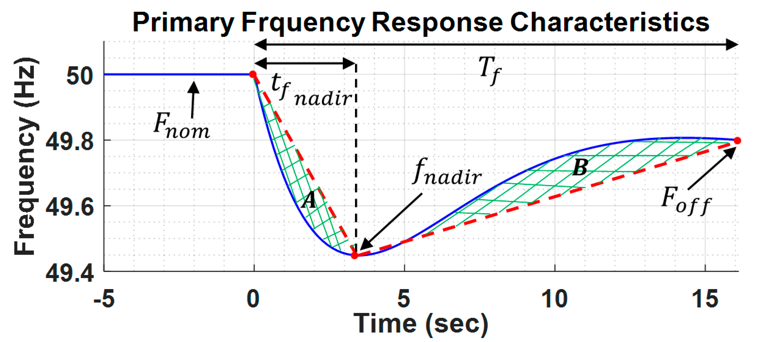
• Consideration 1: The calculation is independent of the exact occurrence of $t_{f_{nadir}}$ with the assumption that it mostly falls in the range of 20 to 40% of $T_f$, which may slightly affect the calculation.
• Consideration 2: The lost area “A” is approximately equal to the gained area “B” in Figure 15, which may slightly affect the energy estimation for the PFR ($E_{S{C}_{PFR}})$. This approximation is quite acceptable in terms of obtaining a rough idea of the total energy requirement for the PFR. This is the case because, eventually, the final sizing will be strictly based on the commercially available SC modules, which will be of appropriate capacitance and voltage ratings with adequate safety factors. Nonetheless, more sophisticated approaches with additional intermediate points or a non-linear model would improve the accuracy of this method, but they would lose out in terms of the superior simplicity and practicality of our method.
• Consideration 3: Due to the linear nature of the TPL characteristic, the peak power demand of PFR $\left(P_{S{C}_{PF{R}_{max}}}\right)$ will occur precisely at the $f_{nadir}$ if only the power contribution due to droop control ($P_{S{C}_{Droop}}$) is considered.
• Consideration 4: The power contribution of RoCoF $(P_{S{C}_{RoCoF}}$) at $t_{f_{nadir}}$ should be considered to be zero because, under normal circumstances, we expect there to be zero RoCoF at $f_{nadir}$ since it is the minima point. Moreover, the contribution of $P_{S{C}_{RoCoF}}$ is negligible at the vicinity of the $f_{nadir}$ point. Therefore, we consider only the droop contribution while estimating $P_{S{C}_{PF{R}_{max}}}$.
• Consideration 5: Do not neglect the $P_{S{C}_{RoCoF}}$ part while calculating the SC Energy rating as there is a signification contribution of RoCoF towards the estimation of $E_{S{C}_{PFR}}$.

Now, the total power expression for PFR ($P_{S{C}_{PFR}}$) with respect to SC storage, considering the effect of dynamic inertia, can be written as:

$$P_{S{C}_{PFR}}=P_{S{C}_{Droop}}+P_{S{C}_{RoCoF}}=\frac{P_{nom}}{F_{nom}}\left[{\left\{\frac{\left(F_{nom}-d{b}_{UF}\right)-f}{k_{UF}}\right\}}_{f<F_{nom}-d{b}_{UF}}+2H_{D}RoCoF\right]$$

(15)

Thus, as per considerations 1, 3 and 4, $P_{S{C}_{PF{R}_{max}}}$ can be calculated for $f=f_{nadir}$ as expressed in Equation (16):

$$P_{S{C}_{PF{R}_{max}}}=P_{S{C}_{Droo{p}_{max}}}=\frac{P_{nom}\left(F_{nom}-d{b}_{UF}-f_{nadir}\right)}{F_{nom}{k}_{UF}}$$

(16)

Similarly, the $E_{S{C}_{PFR}}$ estimation can be performed as per considerations 1, 2, 3 and 5. Basically, energy is the integration of power with respect to time, which is nothing but the area under the power envelope for a specific time interval. Mathematically, this can be written by integrating Equation (15) with respect to time, as shown below:

$$E_{S{C}_{PFR}}=E_{S{C}_{Droop}}+E_{S{C}_{RoCoF}}={{\displaystyle \int }}_0^{T_f}{P}_{S{C}_{PFR}} dt={{\displaystyle \int }}_0^{T_f}\left\{P_{S{C}_{Droop}}+P_{S{C}_{RoCoF}} \right\} dt$$

(17)

where $E_{S{C}_{Droop}}$ and $E_{S{C}_{RoCoF}}$ are the energy contribution due to droop control and RoCoF respectively. Now, $E_{S{C}_{PFR}}$ can be calculated by finding the terms $E_{S{C}_{Droop}}$ and $E_{S{C}_{RoCoF}}$ individually, as shown below:

$$E_{S{C}_{Droop}}={{\displaystyle \int }}_0^{T_f}{P}_{S{C}_{Droop}} dt={\left\{\frac{P_{nom}}{F_{nom}{k}_{UF}}{{\displaystyle \int }}_0^{T_f}\left(F_{nom}-d{b}_{UF}-f\right) dt\right\}}_{f<F_{nom}-d{b}_{UF}}$$

(18)

The term ${{\displaystyle \int }}_0^{T_f}\left(F_{nom}-d{b}_{UF}-f\right)dt$ can easily be graphically solved by finding the area under ABCD of the frequency envelope, as shown in Figure 16, where the lost area corresponding to $d{b}_{UF}$ is represented by the area marked by ADGH.

Mathematically, the area under ABCD can be written as:

$$\begin{array}{c}{{\displaystyle \int }}_0^{T_f}\left(F_{nom}-d{b}_{UF}-f\right) dt=Area \mathrm{ABCD}\hfill \\ \hfill =Area of the triangle \mathrm{ABE}+Area of the triangle \mathrm{BCF}+Area of the rectangle \mathrm{CDEF}\end{array}$$

(19)

$$\begin{array}{cc}Area \mathrm{ABCD}\hfill & =\left[0.5\left\{\frac{t_{f_{nadir}}\left(F_{nom}-f_{nadir}-d{b}_{UF}\right)}{F_{nom}-f_{nadir}}\right\}\left(F_{nom}-f_{nadir}-d{b}_{UF}\right)\right]\hfill \\ & +\left[0.5\left(T_f-t_{f_{nadir}}\right)\left(F_{off}-f_{nadir}\right)\right]+\left[\left(F_{nom}-F_{off}-d{b}_{UF}\right)\left(T_f-t_{f_{nadir}}\right)\right]\hfill \end{array}$$

(20)

After inputting Equation (20) into Equation (18), the expression for $E_{S{C}_{Droop}}$ can be written as:

$$E_{S{C}_{Droop}}=\frac{P_{nom}(Area \mathrm{ABCD})}{F_{nom}{k}_{UF}}$$

(21)

Similarly, the term $E_{S{C}_{RoCoF}}$ can be expressed by considering the average area under IJKL and LMNO of the RoCoF envelope of Figure 16. In addition, as the TPL characteristic has a very sluggish slope, RoCoF is very low in absolute terms ($\left|RoCoF\right|<RC{F}_L$), and the inertia constant is indeed a constant ($H_D=H_H)$.

$$E_{S{C}_{RoCoF}}=\frac{-2H_H{P}_{nom}\left(F_{off}-F_{nom}\right)}{F_{nom}}$$

(22)

From Equation (22), we can see that the value of $E_{S{C}_{RoCoF}}$ is completely independent of the timing of $t_{f_{nadir}}$ and, thus, the inertia energy expenditure depends only upon the deviation of $F_{off}$ from $F_{nom}$.

Finally, the total energy requirement from the SC modules for PFR can be expressed as:

$$E_{S{C}_{PFR}}=\frac{P_{nom}\left\{Area \mathrm{ABCD}-2H_H{k}_{UF}\left(F_{off}-F_{nom}\right)\right\}}{F_{nom}{k}_{UF}}$$

(23)

An example case is solved below for the estimation of $P_{S{C}_{PF{R}_{max}}}$ and $E_{S{C}_{PFR}}$ for the PFR of an under-frequency with the set of parameters for DI control given in Table 3 and with the parameters for Droop control and the TPL method given in

Table 4. Design parameters for Droop control and the proposed TPL method.

Design Parameters	Ratings
$P_{nom}$	10 kW
$d{b}_{UF}$ in PU 1	$\pm$0.003 (Corresponds to 150 mHz)
$k_{UF}$1	0.05
$F_{nom}$	50 Hz
$F_{off}$	49.8 Hz
$T_f$	16.1 s
$f_{nadir}$	49.45 Hz
Ratio of $t_{f_{nadir}}$ to $T_f$	0.214

¹ The setting of these values is in the hands of designer, and is restricted by IEEE 1547-2018 standard.

. Then, for the validation of the proposed TPL methodology, a comparison is made, using the MATLAB Simulink platform, with the benchmark PFR characteristics that have the same sets of parameters as those assumed for the TPL method, as shown in Figure 17.

Example 2.

For the given set of data in Table 4, the value of $P_{S{C}_{PF{R}_{max}}}$can be calculated using Equation (16), as shown below:

$$P_{S{C}_{PF{R}_{max}}}=\frac{\mathrm{10,000}\times \left(50-0.15-49.45\right)}{50\times 0.05}=1600 \mathrm{Watts}$$

Similarly, the value of $E_{S{C}_{PFR}}$ can be calculated by solving Equation (20) and then inputting the solution into Equation (23), as shown below:

$$\begin{array}{ll}Area \mathrm{ABCD}& =\left[0.5\left\{\frac{0.214\times 16.1\left(50-49.45-0.15\right)}{50-49.45}\right\}\left(50-49.45-0.15\right)\right]\\ & +\left[0.5\left(16.1-0.214\times 16.1\right)\left(49.8-49.45\right)\right]\\ & +\left[\left(50-49.8-0.15\right)\left(16.1-0.214\times 16.1\right)\right]=3.3484\end{array}$$

$$E_{S{C}_{PFR}}=\frac{\mathrm{10,000}\left\{3.3484-2\times 9\times 0.05\left(49.8-50\right)\right\}}{50\times 0.05}=\mathrm{14,113.6} \mathrm{Jules}$$

Observations:

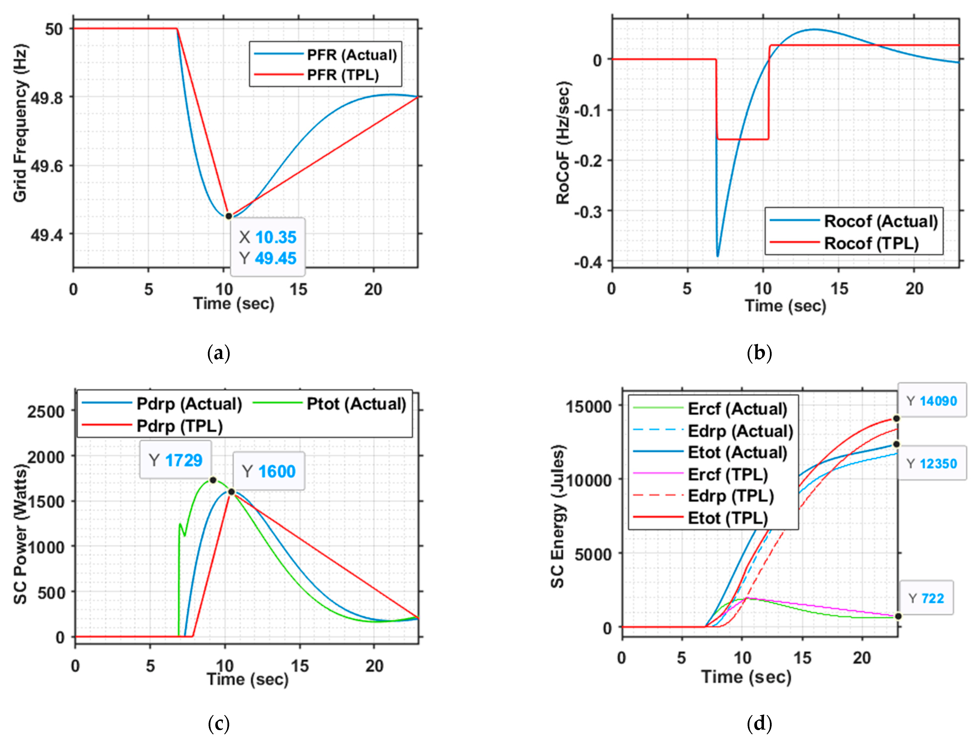
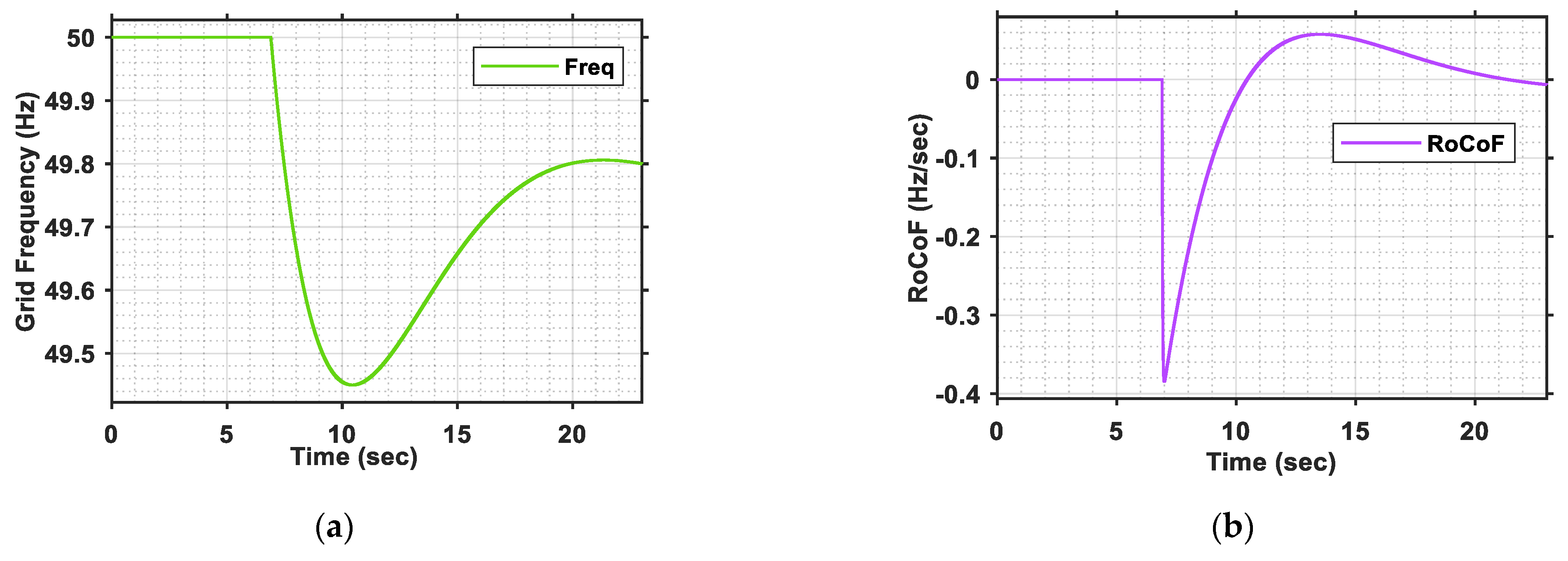
• Firstly, the theoretically calculated value of $P_{S{C}_{PF{R}_{max}}}$ matched exactly with the simulated data of the benchmark case due to “Consideration 3 and Consideration 4”, which were previously mentioned. However, if the contribution of RoCoF was not neglected, there was an error of nearly 100 Watts in the estimation of $P_{S{C}_{PF{R}_{max}}}$, which was small and acceptable. This error occurred because, in the case of actual PFR characteristics, the $P_{S{C}_{PF{R}_{max}}}$ mostly occurred slightly before the $t_{f_{nadir}}$ as the initial contribution of $P_{S{C}_{RoCoF}}$ was greater due to the high starting RoCoF.
• Secondly, the theoretically calculated value of $E_{S{C}_{PFR}}$ matched exactly with the simulated data for TPL characteristics. However, the simulated benchmark data were almost 12.5% smaller than those of the TPL characteristics data due to “Consideration 1 and Consideration 2”, which were mentioned previously. The main cause of the error was the overly sluggish slope of the TPL characteristics from the $t_{f_{nadir}}$ point to $T_f$. Additional intermediate points can help in reducing the error, but this is ultimately a trade-off between simplicity and accuracy.
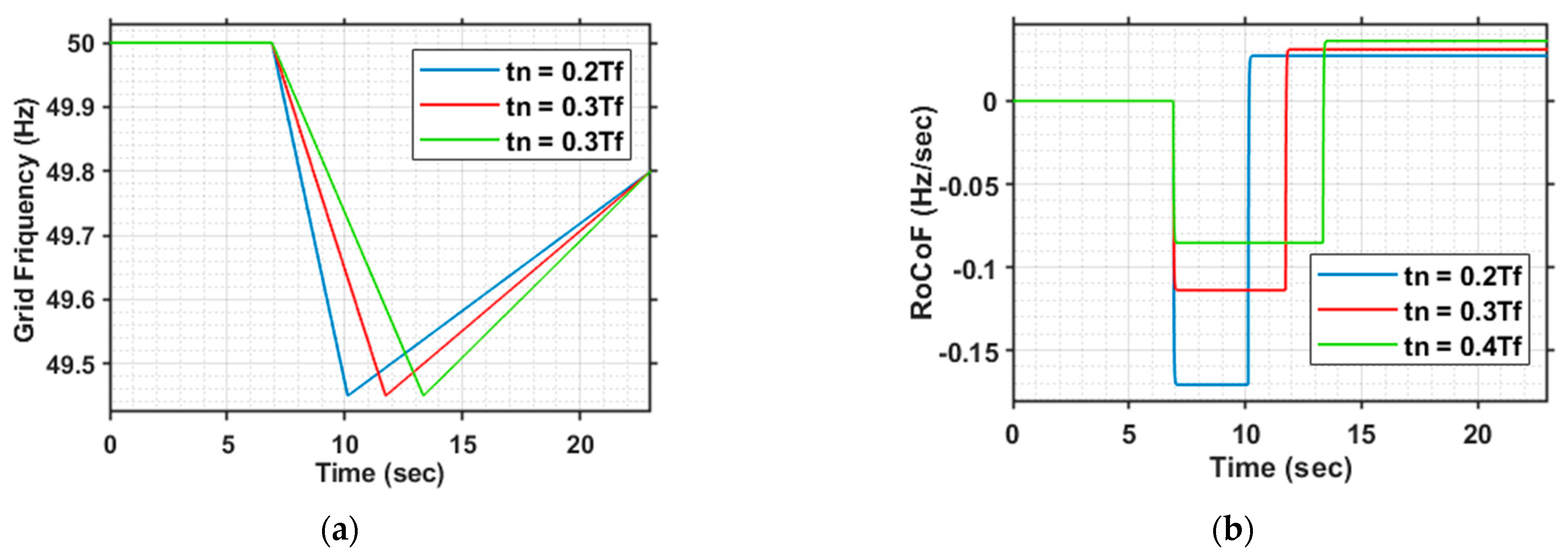
• Thirdly, the $E_{S{C}_{RoCoF}}$ of the TPL characteristics matched exactly with that of the benchmark PFR characteristics as it was independent of the timing of $t_{f_{nadir}}$ and was a function of the difference between $F_{off}$ and $F_{nom}$.

Although, there were some small amounts of errors, in the cases of both the power and energy estimation of PFR using the TPL method, the results were perfectly acceptable, as the final design should be based on the commercially available SC module of the nearly calculated rating with some safety factors taken into account. In fact, there was a difference when instantaneous values were compared, but we did not take this into consideration as it will not affect the final design.

The TPL method was also verified for different positions of $t_{f_{nadir}}$ with similar values of $f_{nadir}$, and their results were compared in the MATLAB Simulink environment, as shown in Figure 18. Below are some of the observations:

• $P_{S{C}_{PF{R}_{max}}}$ was independent of the timing of $t_{f_{nadir}}$.
• $E_{S{C}_{RoCoF}}$ was independent of $t_{f_{nadir}}$ and $f_{nadir}$.
• There was slight difference in the values of $E_{S{C}_{Droop}}$ for all three cases due to differences in the area under ABCD, which resulted in a slight difference in total energy, but the results were perfectly acceptable. Therefore, we can assume a $t_{f_{nadir}}$ value around 0.2–0.4 of $T_f$ when the former specification is not available.

5.3. Finalization of the SC Overall Rating

Once the power and energy rating of the SC storage system corresponding to both the SIR and the PFR were calculated, the final effective ratings to satisfy both objectives could be calculated as shown in the equations below:

$$P_{S{C}_{eff}}\ge max\left(P_{S{C}_{SI{R}_{max}}}, P_{S{C}_{PF{R}_{max}}}\right)$$

(24)

$$E_{S{C}_{eff}}\ge \frac{E_{S{C}_{PFR}}}{\beta }$$

(25)

where $\beta$ is the maximum allowable depth of discharge, which was mostly up to around 80% of its rated SOC. This was the case because, unlike BESS, the SC voltage varied largely with the variation of the SOC. Although, unlike BESS, the SC could be discharged to zero voltage and could be brought back to life, the restriction in the level of discharge was mostly essential in order to avoid high gain requirement of the SC-PPS.

Now, for the system under consideration discussed in Examples 1 and 2, the $P_{S{C}_{eff}}$ and $E_{S{C}_{eff}}$ could be calculated using Equations (24) and (25), as shown below:

$$P_{S{C}_{eff}}\ge max\left(1885 \mathrm{Watts}, 1600 \mathrm{Watts}\right) \approx 2 \mathrm{kW}$$

$$E_{S{C}_{eff}}\ge \frac{\mathrm{14,113.6} \mathrm{Jules}}{0.8}\ge \mathrm{17,642} \mathrm{Jules}$$

In Figure 19, a brief flowchart is given, which discusses the step-by-step process of the designing and sizing of the SC storage for the proposed PSCT. Once the $P_{S{C}_{eff}}$ and $E_{S{C}_{eff}}$ are decided, the selection of capacitance $\left(C_{SC}\right)$ and $\left(V_{SC}\right)$ rating of SC should be conducted wisely to meet the estimated $P_{SC\_eff}$ and $E_{SC\_eff}$ requirements. Here, the authors found that by connecting three numbers of commercially available SC units (BMOD0058 E016 B02: 58 F, 16 V, 170 A(peak)) in series the desired performance can be achieved. The corresponding $C_{SC}$ and $V_{SC}$ of the series connection could be calculated to be 19.3 F and 48 V, respectively, with an energy storing capability of up to 22.2 kJ. Considering that the SC is not allowed to discharge below 20 V (which corresponds to nearly 20% of the rated SOC) to avoid high gain requirement issues, we could still extract nearly 18.4 kJ of energy if fully charged, which was indeed not a bad figure and was more than the requirement. Thus, if integrated to a PV system of 10 kWp, this method will be capable of emulating the dynamic synthetic inertia in the range of 2 to 9 s based on the RoCoF, which was much better and flexible than the synchronous generators in scale. This can be a cheap solution to provide some inertia to the PV system, costing no more than $\mathrm{GBP} 300 \mathrm{or} \mathrm{INR} \mathrm{27,000}$. In fact, although the bust power rating of the selected SC module set was much higher than the required power rating, the SC-PPS was designed for 2 kW only due to the design constraints.

6. Verification of the Concept Subjected to Case Studies Using MATLAB/OPAL RT

In this section, a thorough case study is carried out for both SIR and PFR to verify the proposed PSCT and the associated controls, taking into account the estimated rating of the SC based on the proposed sizing methodologies.

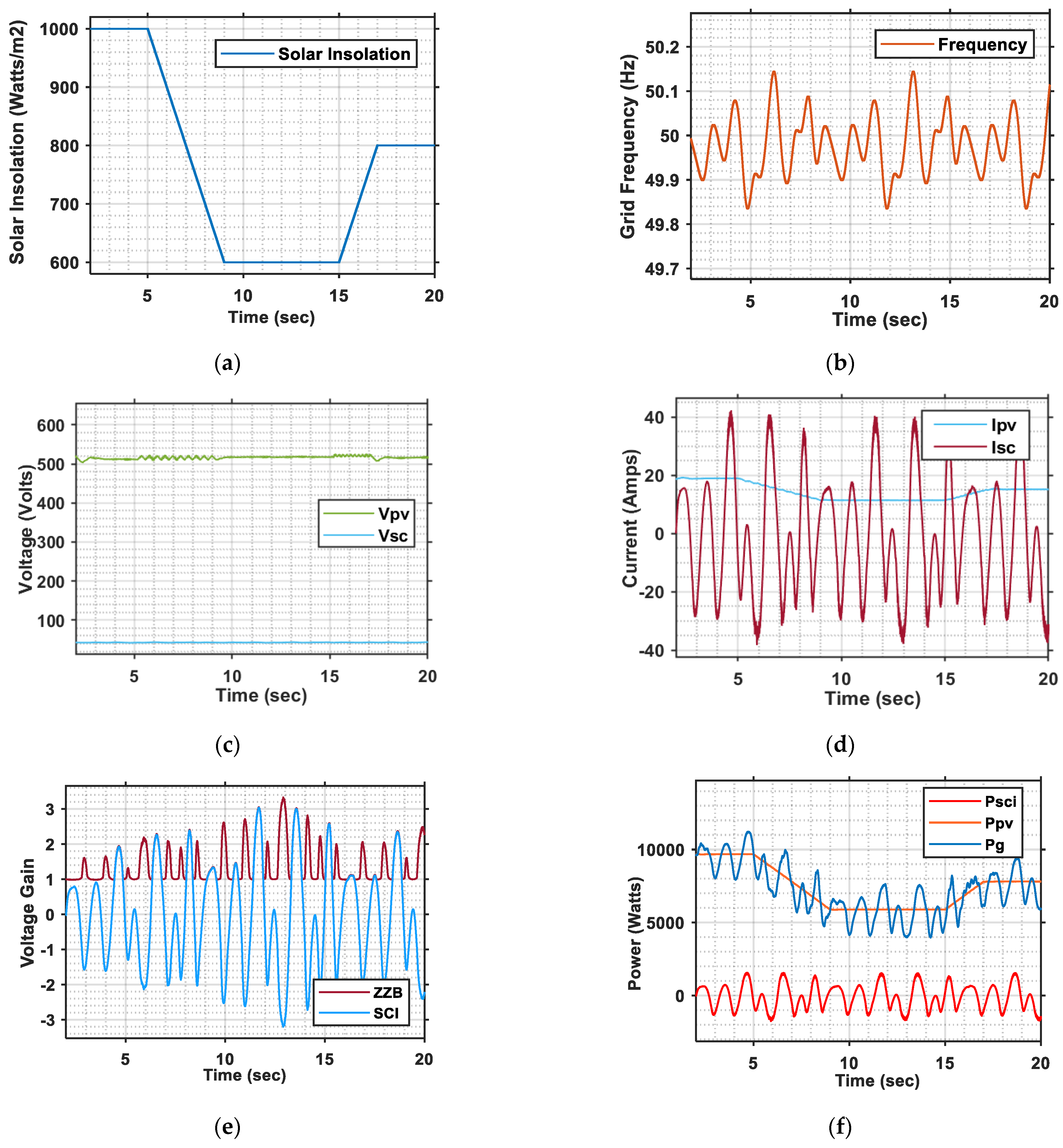
6.1. Case Studies to Verify SIR Only for Small-Frequency Fluctuations

In this case, the system under consideration, as mentioned in Table 1, was subjected to a small-frequency fluctuation of less than $\pm 0.03 \mathrm{PU}$. For the implemented control and the sets of parameters of Table 3 and Table 4, the responses are compared in Figure 20 for four different cases of inertia mentioned in

Table 5. Case Studies for SIR.

Case Studies	Parameters
Case 1 1	Constant $H=2$ s
Case 2 1	Constant $H=6$ s
Case 3	Constant $H=9$ s
Case 4	Proposed Dynamic Inertia Concept $(2 \mathrm{s}\le H_D\le 9 \mathrm{s}$)

¹ Comparable to the range of classical rotating generators in scale.

to justify the superiority of the proposed dynamic inertia control over its constant inertia-based counterparts.

It can be seen that in low-RoCoF situations, case 3 and case 4 perform better compared to case 1 and case 2 due to high inertia emulation. However, during the comparatively high-RoCoF period, case 3 saturates the SC power output to 2 kW, whereas case 4 modulates the output power as per the RoCoF profile, without saturation, through the use of the dynamic inertia concept. Thus, this proves the pre-eminence of the dynamic inertia emulation method over other constant inertia emulation methods.

The dynamics of the proposed PSCT and the associated control were also verified for the case of renewable intermittencies. An example case of involved the variation of the insolation from 1000 W/m² to 600 W/m² before being increased and settled at 800 W/m² (at a rate of 100 W/m²/s for fast irradiance transient) was simulated and verified for the case of SIR. The corresponding results are shown in Figure 21 for the reader’s convenience. From the results, it is clear that the control of PV MPPT is perfectly decoupled from the control of SC-PPS.

Below are the some of the findings from the simulation results of the case study with the renewable intermittencies:

• The proposed control ensured that the PV MPPT control was fully decoupled from the SC-PPS control, which was related to frequency response services.
• SIR was provided seamlessly irrespective of variations in the MPPT power, in accordance with the variation in solar insolation under consideration, and vice versa.
• Although there was hardly any change in MPPT voltage profile, the SC-PPS stage control responded to changes in the series PV current and regulated its output voltage to meet the required power exchange, thus proving the resiliency of our proposed control against the rapid change in the master source.

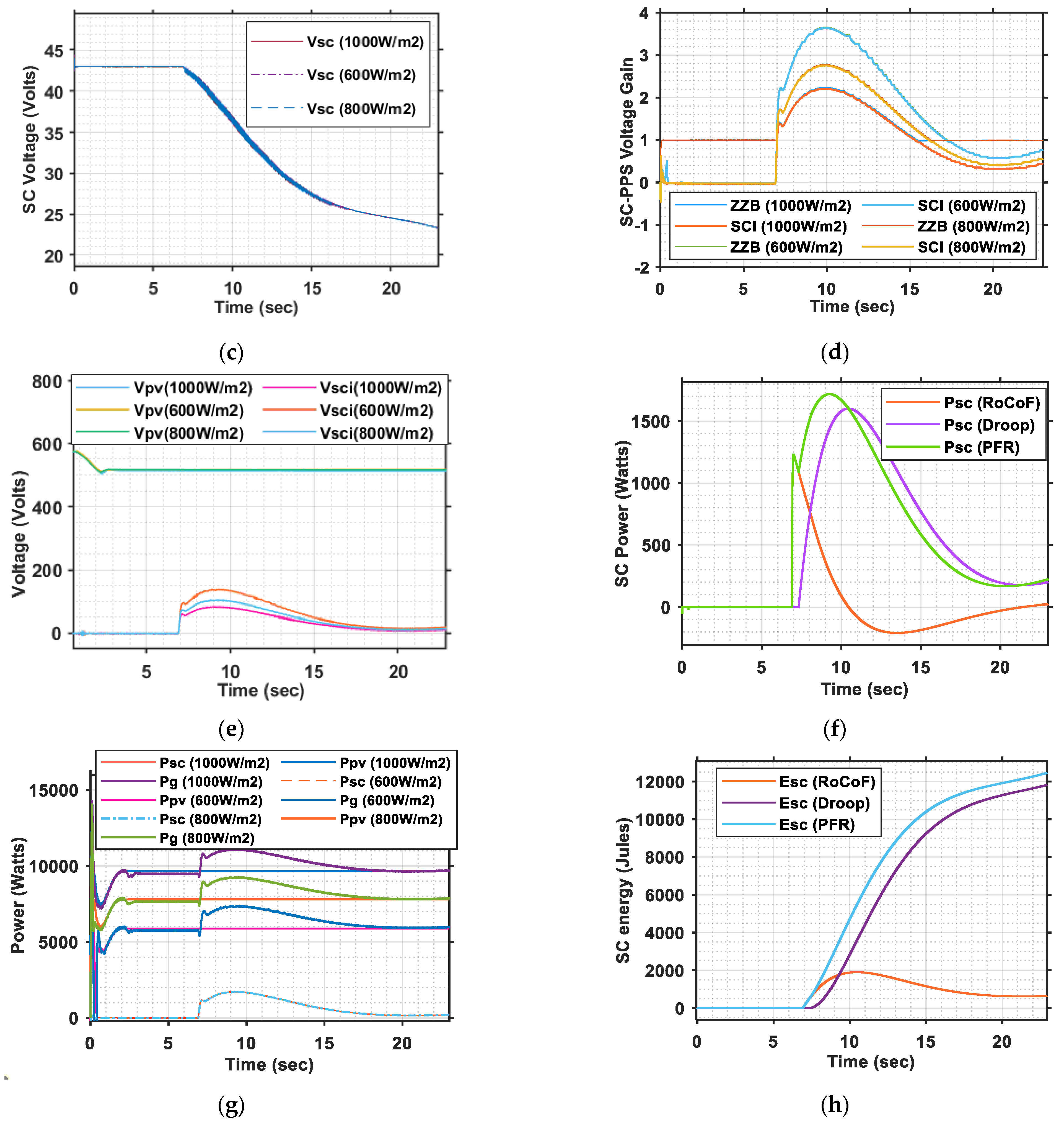
6.2. Case Studies to Verify PFR for Under-Frequency Events without Small-Frequency Fluctuations

In this case, the system under consideration in Table 1 was subjected to an under-frequency event as per the parameters in Table 4, without any low-frequency fluctuations, and the corresponding PFR were investigated, as shown in Figure 22, for different solar insolation levels, as mentioned in

Table 6. Case Studies for PFR without any low-frequency fluctuation in the PFR envelope.

Case Studies	Solar Insolation
Case 1	1000 Watts/m2
Case 2	800 Watts/m2
Case 3	600 Watts/m2

.

As can be seen, for all the three cases, the SC power outputs were the same and were independent of the PV output. During periods of high solar insolation levels, as the PV current was comparatively high, the voltage gain requirement of the SC-PPS was also low and was below a gain level of three. However, during periods of low insolation levels, the series PV current was relatively low; therefore, to generate the required power output, the control increased the output voltage of SC-PPS with a gain requirement as high as nearly four. The ZZB played a very important role here in terms of providing the required voltage gain, which was almost impossible with a conventional boost converter.

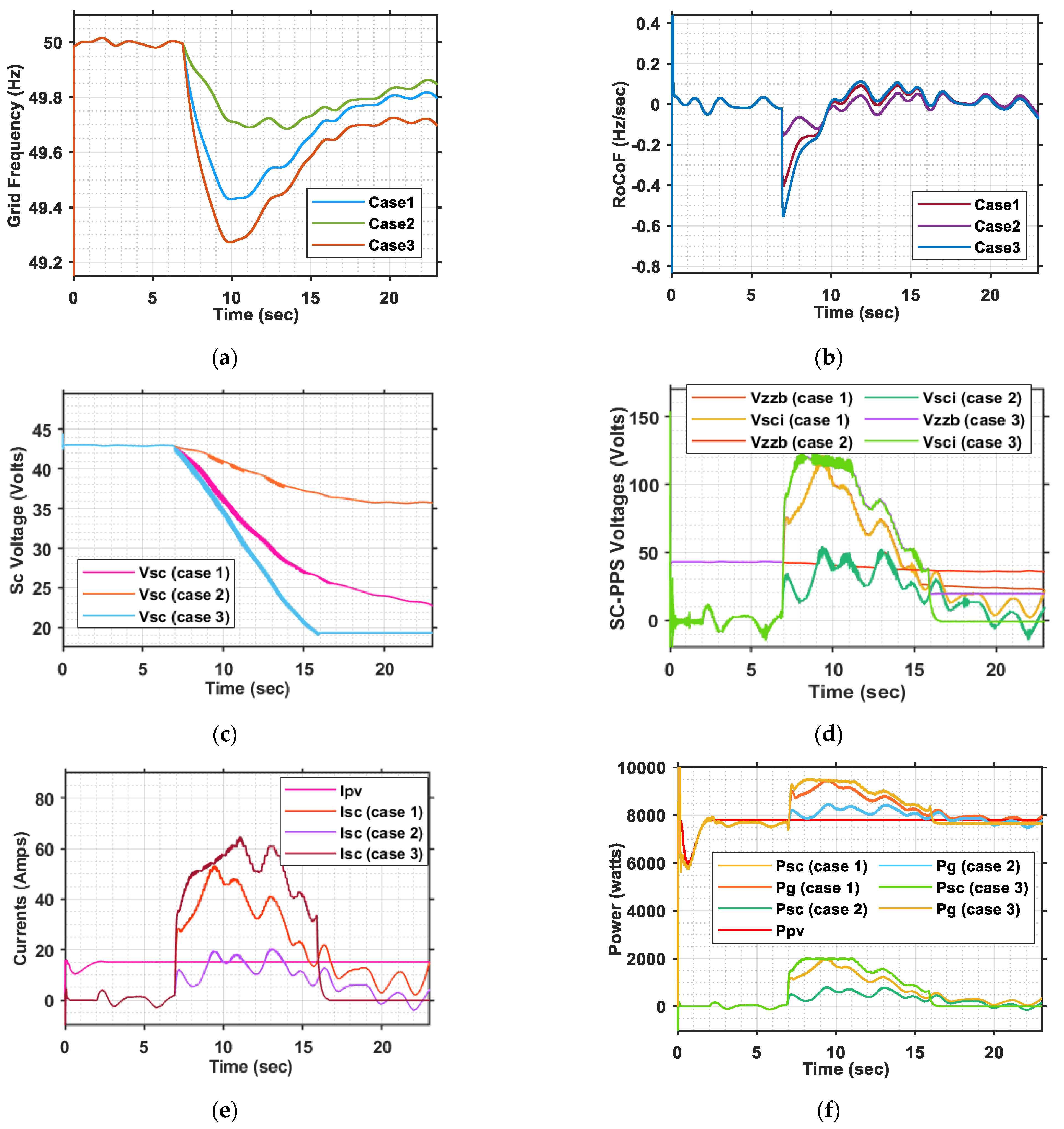
6.3. Case Studies to Verify PFR for Under-Frequency Events with Small-Frequency Fluctuations

In this case, the system under consideration was subjected to both under-frequency events, with a low-frequency oscillation over its envelope. The corresponding system responses were investigated, as shown in Figure 23, for three different scenarios of severity for under-frequency events, in terms of the depth of $f_{nadir}$, the timing of $t_{f_{nadir}}$, and the $F_{off}$ values, as mentioned in

Table 7. Case Studies for PFR with low-frequency fluctuation in the PFR envelope.

Case Studies	Parameters for Frequency Events
Case 1	$f_{nadir}=49.45$ Hz, $t_{f_{nadir}}=0.214T_f$, $F_{off}=49.8 \mathrm{Hz}$
Case 2	$f_{nadir}=49.7$ Hz, $t_{f_{nadir}}=0.34T_f$, $F_{off}=49.85 \mathrm{Hz}$
Case 3	$f_{nadir}=49.3$ Hz, $t_{f_{nadir}}=0.204T_f$, $F_{off}=49.7 \mathrm{Hz}$

.

The results show that, for the low- and medium-type severity cases of under-frequency events, such as case 1 and case 2, the power and/or energy demands were within the designed saturation limit. However, during intense under-frequency events such as case 3, mostly due to the sudden increase in load caused by the power demand being more than 2 kW for some interval of time, the control saturated its output to the design limit. This was acceptable, as case 3 fell outside of the design specifications.

The duration of the fault ($T_f$) and the solar insolation were considered to be 16.1 s and 800 Watts/m², respectively, for all three cases.

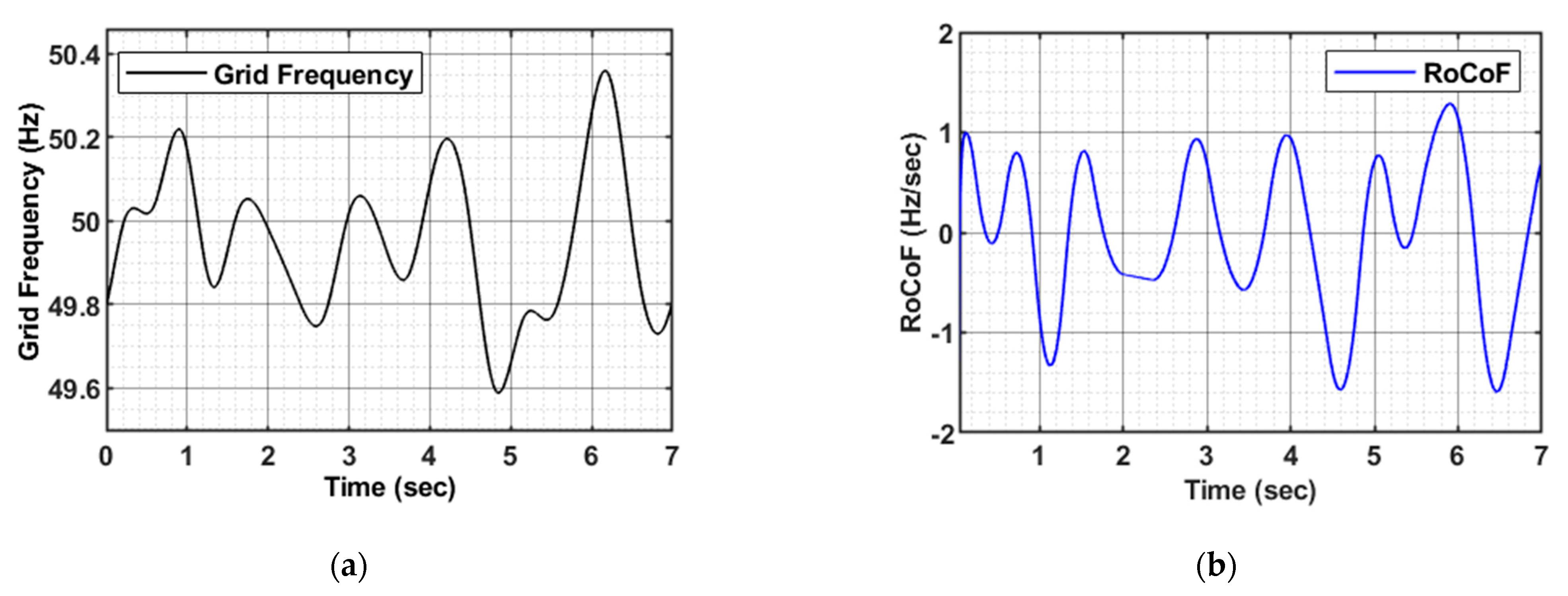
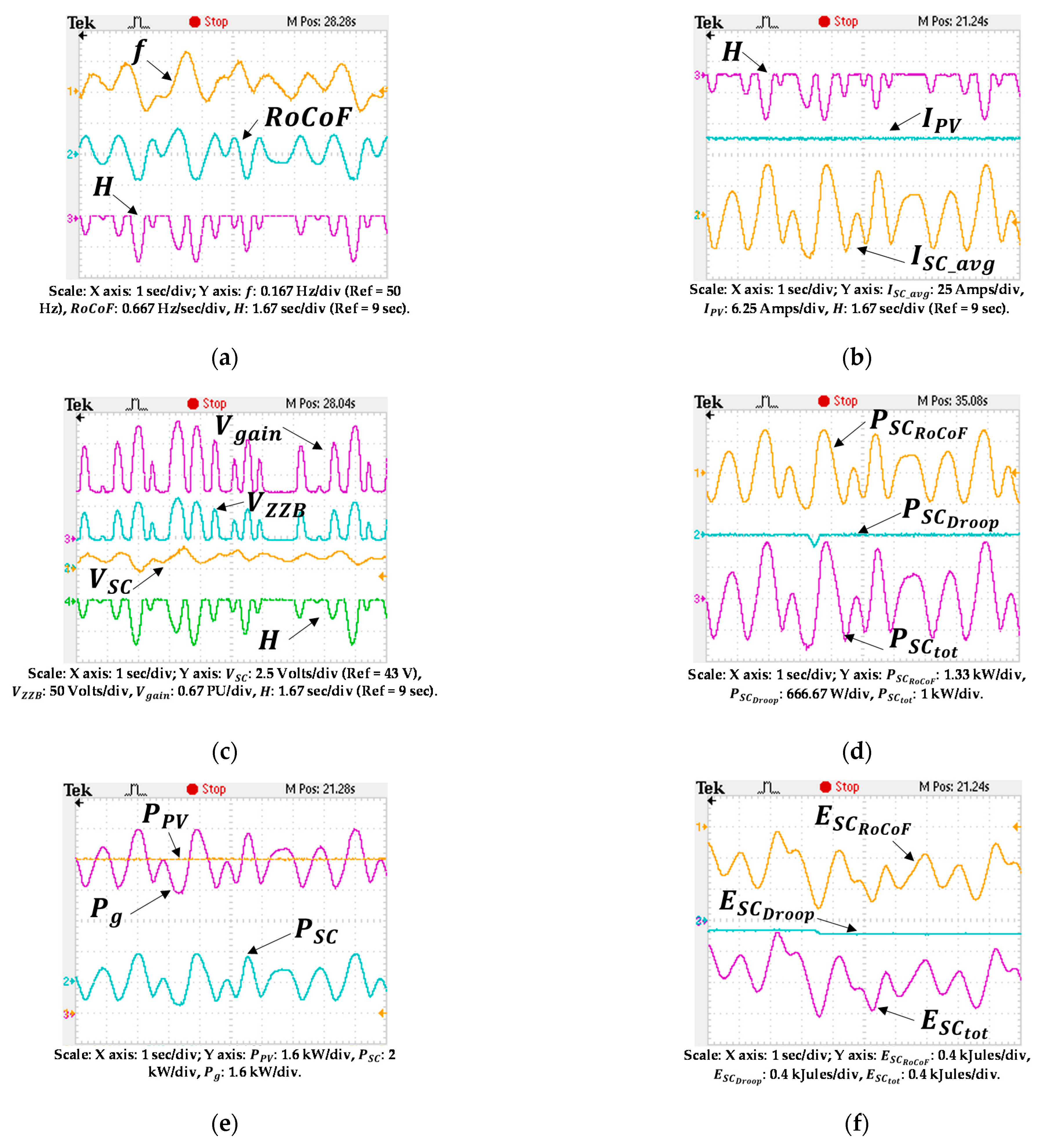
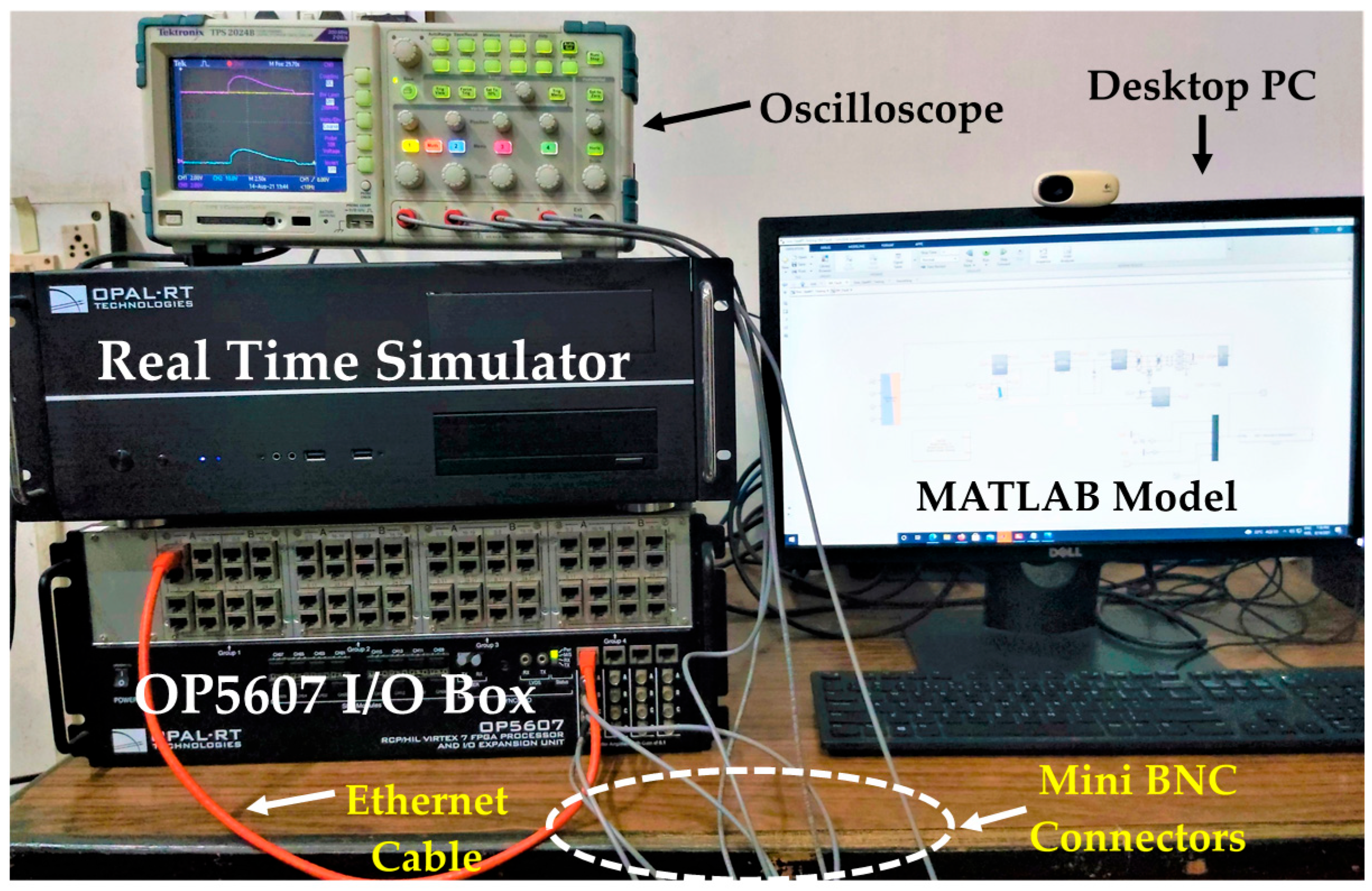
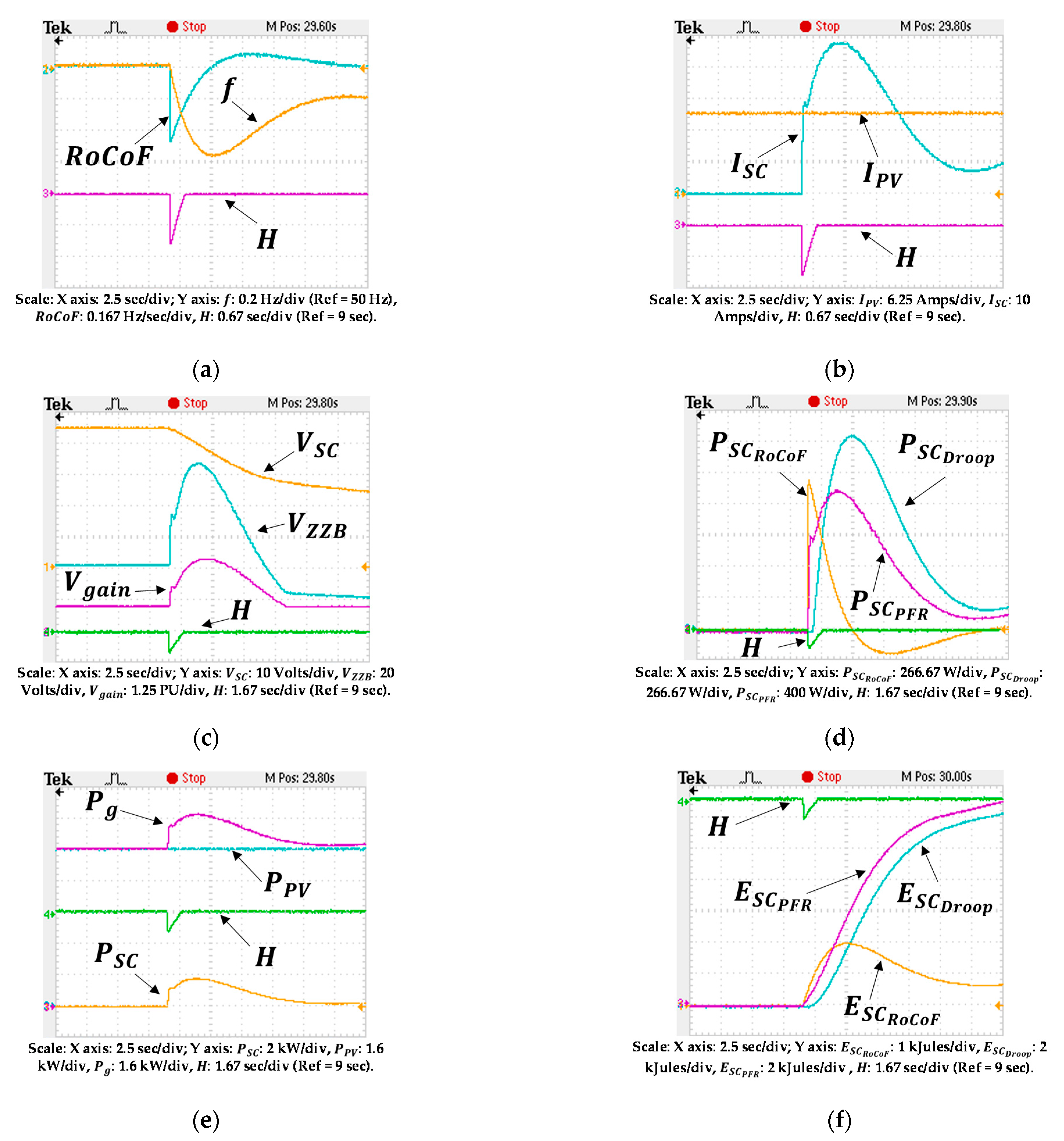
6.4. Validation through OPAL RT Test Bed

For confirmation, the concept proposed in this article was also validated through the OPAL-RT-based Real-Time Simulation (RTS) platform for numerous case studies. The arrangement of the RTS test bed platform is shown in Figure 24. The basic functional units, which complete the test bed, were a Processing Unit, an I/O expansion Unit, a Host PC/Desktop and an Oscilloscope. The processing unit used real-time simulators, which were mostly supported by a Redhat Linux-based real-time operating system. An Ethernet cable fulfilled the communication protocol between the host PC and the real-time processing unit. The OP5607 I/O box was an I/O expansion unit that runs on the Vertex-7 FPGA platform with 96 I/Os distributed on both the front and back side of the chassis. An ethernet-straight cable connected the processing unit with the I/O box, and a set of mini BNC connectors helped in transferring the signal from the I/O box to the oscilloscope. The associated control system and the power circuit were first modelled in the MATLAB R2019b platform and then linked to the OPAL-RT real-time processing unit through the RT-Lab GUI for performance verification.

Each of the three sets of pre-discussed case studies correspond to low-frequency and under-frequency events, which, considered both separately and also as a simultaneous event, were thoroughly verified using the OPAL RT real-time platform. Their responses were validated through comparison with the corresponding simulation results. As an example, a few important results of one of the cases from each of the pre-discussed case studies, as mentioned in

Table 8. Example cases for various types of frequency events verified in the OPAL RT real-time simulation environment.

Event Types	Example Cases
Low-Frequency Oscillation alone	Case study 1: Case 4 of Table 5
Under-Frequency Event alone	Case study 2: Case 2 of Table 6
Both as a simultaneous event	Case study 3: Case 1 of Table 7

, are shown in Figure 25, Figure 26 and Figure 27, respectively, for the reader’s convenience.

The severity of low-frequency oscillation was considered to be low for case study 3 as compared to case study 1.

Below are several considerations for all the three cases of frequency events mentioned in Table 8.

• The severity of low-frequency oscillation was considered low for Case study 3 as compared to Case study 1.
• The Solar Insolation, for all the case studies, was considered to be 800 Watts/m².
• The initial SC voltage was 43 V for all the cases and, for Case study 1, 43 V was taken as the reference for plotting of the SC voltage profile.
• The emulated inertia profile was considered as a reference for all the real-time results to understand the system response with respect to the occurrence of the event.
• The scaling of the measuring entities was selected in such a way that the effect of noise in the BMC connector could be minimized.
• For the frequency profile, 50 Hz was taken as a reference for plotting.
• For the inertia profile, 9 s was taken as a reference for plotting.

Below are some of observations regarding the results obtained in Figure 25:

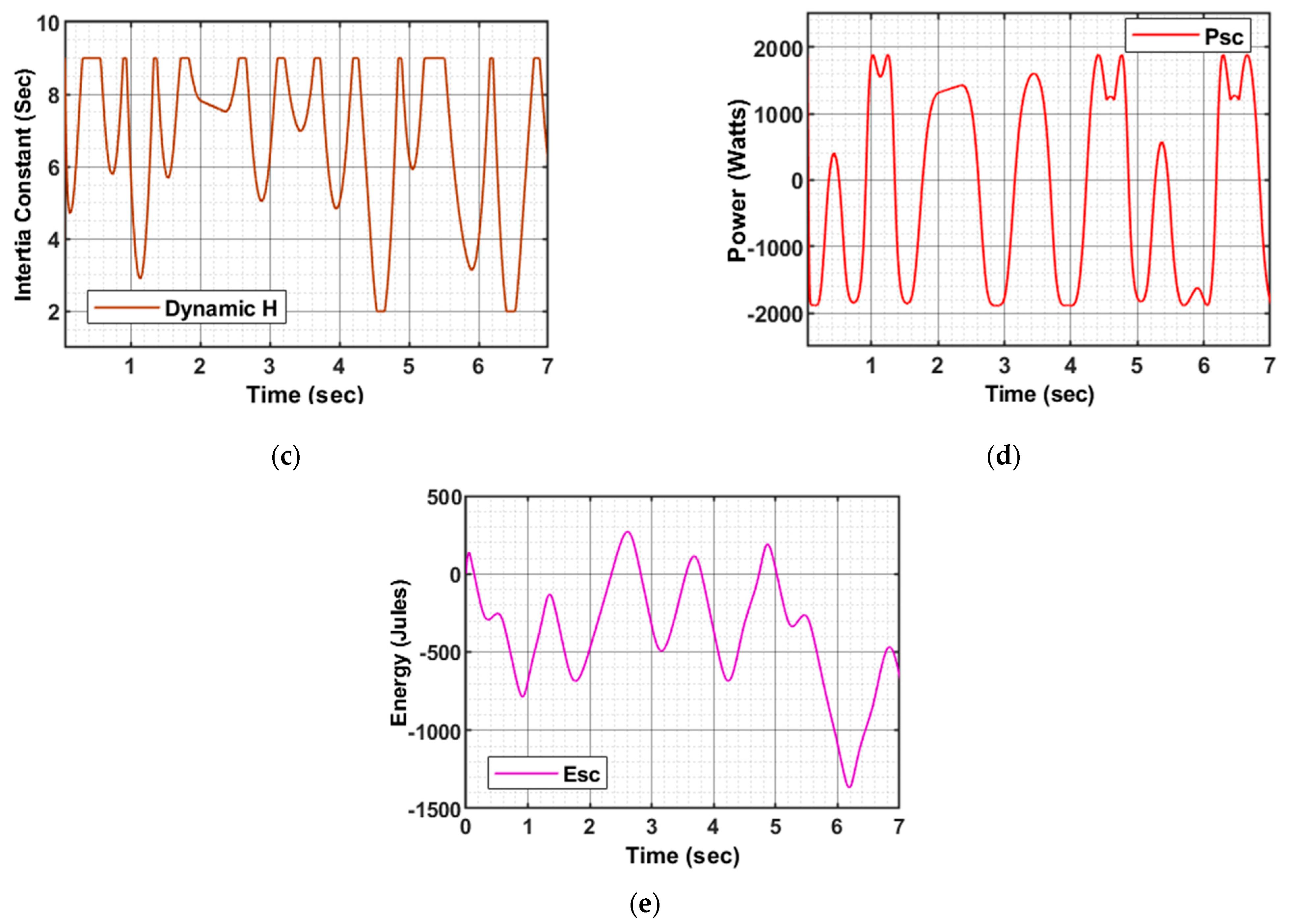
• The emulated inertia constant (PU) varied between 9 and 6.5 s.
• The variation in SC voltage profile was almost negligible.
• The maximum voltage gain requirement of the ZZB was nearly 2.5.
• The peak average current of the SC was nearly $\pm$43 A.
• The PV current remained unaffected with an MPPT current of nearly 15.8 A.
• The contribution of the Droop control was almost zero.
• The peak SC power requirement was nearly $\pm$1.8 kWatts.
• The total grid power was the sum of the PV MPPT power and the SC output power.
• The SC energy requirement over a cycle of a few seconds was almost zero.

Below are some of observations regarding the results obtained in Figure 26:

• The emulated inertia constant (PU) dropped down to almost 7.9 s from 9 s precisely at the moment of the frequency event due to the high RoCoF.
• The SC experienced a large variation of voltage from 43 to 25 V.
• The maximum voltage gain requirement of the ZZB was nearly 2.9. (operated at unity gain before the event).
• The peak average current of the SC was nearly 48 A.
• The PV current remained unaffected with an MPPT current of nearly 15.8 A.
• The contribution of the Droop control was prevalent over the RoCoF control.
• The peak SC power requirement was nearly 1.8 kWatts.
• The SC energy requirement was found to be nearly 13 kJules.
• The total grid power was the sum of the PV MPPT power and the SC output power.

Below are some observations regarding the results obtained in Figure 27:

• The emulated inertia constant (PU) dropped down to almost 7.3 s from 9 s precisely at the moment of the frequency event due to the high RoCoF.
• The SC experienced a large variation in voltage from 43 to 25 V.
• The maximum voltage gain requirement of the ZZB was nearly 3.6 (operated close to unity gain before the under-frequency event).
• The peak average current of SC was nearly 52 A.
• The PV current remained unaffected with an MPPT current of nearly 15.8 A.
• The contribution of the Droop control prevailed over the RoCoF control.
• The peak SC power requirement was nearly 2 kWatts.
• The SC energy requirement was nearly 12.4 kJules.

7. Conclusions

In this study, a novel cascaded topology for a PV super-capacitor was proposed to address issues related to grid frequency services through a naturally zero-inertia-based PV system with the help of a small SC-based storage unit to emulate synthetic inertia. The idea was to drastically reduce the gain requirement of the interfacing converters for the charge control of a low-voltage-profile-based SC storage unit. It was observed that a simple non-isolated bidirectional bipolar power-processing stage arrangement of a voltage gain capability of nearly four can be used to interface an SC storage unit whose voltage may fall in the range of 15 to 35 times less than the nominal PV MPPT voltage. This concept of series voltage injection with the proposed control has the potential to be used to emulate some synthetic inertia in a 10 kWp PV system with an additional cost of only GBP $300 \mathrm{or} \mathrm{INR} \mathrm{27,000}$. Nonetheless, the proposed configuration also has application capabilities in scenarios involving power levels ranging from a few hundreds of kWp to a few MWp due to its modularity structure.

The proposed concept of Dynamic Inertia Emulation has the proficiency to provide variable synthetic inertia in the range of 2 to 9 s, which is either equal to or better than the classical alternators in terms of scale. The flexibility in the variable inertia emulation method can address a large range of Rate of Change of Frequency values, up to almost $\pm$2 Hz/s, just with the help of a limited storage of up to 2 kW ramping capability with negligible net energy demand over a period of few seconds. The suggested Three-Point Linearization approach for sizing of the SC storage unit to obtain the Primary Frequency Response proves its novelty, and it offers the least amount of compromise in terms of both simplicity and accuracy when the exact profile of the frequency event is unknown to the designer. The proposed sizing methodology estimated that the series connection of three numbers of commercially available SC units (BMOD0058693E016 B02: 58F, 16V, 170A (peak)) can easily fulfill the desired performance requirements with an energy-storing capability of almost 22.2 kJ. Finally, the concept was validated with the help of a MATLAB simulation model and a Real-Time Simulation test bed based on the OPAL RT platform for various case studies. Nevertheless, in addition to the conventional and widely adopted grid-following control approach, the proposed PSCT concept can also be explored for grid-forming control systems, such as virtual synchronous machines. However, the authors consider this to be a very good research direction for future work.

References

1. Capacity-and-Generation. Available online: https://www.irena.org/Statistics/View-Data-by-Topic/Capacity-and-Generation (accessed on 2 July 2021).
2. GREENING THE GRID: Pathways to Integrate 175 Gigawatts of Renewable Energy into India’s Electric Grid, Vol. I—National Study. Available online: https://www.nrel.gov/docs/fy17osti/68530.pdf (accessed on 2 July 2021).
3. United Nations Framework Convention on Climate Change. Available online: https://en.wikipedia.org/wiki/United_Nations_Framework_Convention_on_Climate_Change (accessed on 9 August 2021).
4. Rajan, R.; Francis, M.F.; Yang, Y. Primary frequency control techniques for large-scale PV-integrated power systems: A review. Renew. Sustain. Energy Rev. 2021, 144, 110998. [Google Scholar] [CrossRef]
5. Hartmann, B.; Vokony, I.; Táczi, I. Effects of decreasing synchronous inertia on power system dynamics—Overview of recent experiences and marketisation of services. Int. Trans. Electr. Energy Syst. 2019, 29, e12128. [Google Scholar] [CrossRef] [Green Version]
6. Black System South Australia 28 September 2016—Final Report. Available online: http://www.aemo.com.au/-/media/Files/Electricity/NEM/Market_Notices_and_Events/Power_System_Incident_Reports/2017/Integrated-Final-Report-SA-Black-System-28-September-2016.pdf (accessed on 12 July 2021).
7. Delille, G.; François, B.; Malarange, G. Dynamic frequency control support: A virtual inertia provided by distributed energy storage to isolated power systems. In Proceedings of the 2010 IEEE PES Innovative Smart Grid Technologies Conference Europe (ISGT Europe), Gothenburg, Sweden, 11–13 October 2010; pp. 1–8. [Google Scholar]
8. Agha, M.M.; Hajar, A. A new approach for optimal sizing of battery energy storage system for primary frequency control of islanded Microgrid. Int. J. Electr. Power Energy Syst. 2014, 54, 325–333. [Google Scholar]
9. Wu, D.; Tang, F.; Dragicevic, T.; Guerrero, J.M.; Vasquez, J.C. Coordinated Control Based on Bus-Signaling and Virtual Inertia for Islanded DC Microgrids. IEEE Trans. Smart Grid 2015, 6, 2627–2638. [Google Scholar] [CrossRef] [Green Version]
10. Miguel, R.G.; Rafael, C.; Jorge, C.; Malik, O.P. Placement and sizing of battery energy storage for primary frequency control in an isolated section of the Mexican power system. Electr. Power Syst. Res. 2018, 160, 142–150. [Google Scholar]
11. Engels, J.; Claessens, B.; Deconinck, G. Combined Stochastic Optimization of Frequency Control and Self-Consumption with a Battery. IEEE Trans. Smart Grid 2019, 10, 1971–1981. [Google Scholar] [CrossRef] [Green Version]
12. Zhang, Y.J.A.; Zhao, C.; Tang, W.; Low, S.H. Profit-Maximizing Planning and Control of Battery Energy Storage Systems for Primary Frequency Control. IEEE Trans. Smart Grid 2018, 9, 712–723. [Google Scholar] [CrossRef] [Green Version]
13. Lee, D.; Wang, L. Small-Signal Stability Analysis of an Autonomous Hybrid Renewable Energy Power Generation/Energy Storage System Part I: Time-Domain Simulations. IEEE Trans. Energy Convers. 2008, 23, 311–320. [Google Scholar] [CrossRef]
14. Tam, K.; Kumar, P.; Foreman, M. Enhancing the utilization of photovoltaic power generation by superconductive magnetic energy storage. IEEE Trans. Energy Convers. 1989, 4, 314–321. [Google Scholar] [CrossRef]
15. Ibrahim, H.; Ilinca, A.; Perron, J. Energy storage systems—Characteristics and comparisons. Renew. Sustain. Energy Rev. 2008, 12, 1221–1250. [Google Scholar] [CrossRef]
16. Sutanto, D.; Cheng, K.W.E. Superconducting magnetic energy storage systems for power system applications. In Proceedings of the International Conference on Applied Superconductivity and Electromagnetic Devices, Chengdu, China, 25–27 September 2009. [Google Scholar]
17. Sangwongwanich, A.; Yang, Y.; Blaabjerg, F.; Sera, D. Delta Power Control Strategy for Multistring Grid-Connected PV Inverters. IEEE Trans. Ind. Appl. 2017, 53, 3862–3870. [Google Scholar] [CrossRef] [Green Version]
18. Zarina, P.P.; Mishra, S.; Sekhar, P.C. Exploring frequency control capability of a PV system in a hybrid PV-rotating machine-without storage system. Int. J. Electr. Power Energy Syst. 2014, 60, 258–267. [Google Scholar] [CrossRef]
19. Hoke, A.F.; Shirazi, M.; Chakraborty, S.; Muljadi, E.; Maksimovic, D. Rapid Active Power Control of Photovoltaic Systems for Grid Frequency Support. IEEE J. Emerg. Sel. Top. Power Electron. 2017, 5, 1154–1163. [Google Scholar] [CrossRef]
20. Hoke, A.F.; Maksimovic, D. Active power control of photovoltaic power systems. In Proceedings of the IEEE Conference on Technologies for Sustainability (SusTech), Portland, OR, USA, 1–2 August 2013. [Google Scholar]
21. Crăciun, B.; Kerekes, T.; Séra, D.; Teodorescu, R. Frequency Support Functions in Large PV Power Plants with Active Power Reserves. IEEE J. Emerg. Sel. Top. Power Electron. 2014, 2, 849–858. [Google Scholar] [CrossRef]
22. Lyu, X.; Zhao, X.; Zhao, J. A coordinated frequency control strategy for photovoltaic system in micro grid. J. Int. Counc. Electr. Eng. 2018, 8, 37–43. [Google Scholar] [CrossRef] [Green Version]
23. Sekhar, P.C.; Mishra, S. Storage Free Smart Energy Management for Frequency Control in a Diesel-PV-Fuel Cell-Based Hybrid AC Microgrid. IEEE Trans. Neural Netw. Learn. Syst. 2016, 27, 1657–1671. [Google Scholar] [CrossRef]
24. Soni, N.; Doolla, S.; Chandorkar, M.C. Improvement of Transient Response in Microgrids Using Virtual Inertia. IEEE Trans. Power Deliv. 2013, 28, 1830–1838. [Google Scholar] [CrossRef]
25. Kerdphol, T.; Watanabe, M.; Hongesombut, K.; Mitani, Y. Self-Adaptive Virtual Inertia Control-Based Fuzzy Logic to Improve Frequency Stability of Microgrid with High Renewable Penetration. IEEE Access 2019, 7, 76071–76083. [Google Scholar] [CrossRef]
26. Guo, K.; Tang, Y.; Fang, J. Exploration of the Relationship Between Inertia Enhancement and DC-Link Capacitance for Grid-Connected Converters. In Proceedings of the IEEE 4th Southern Power Electronics Conference (SPEC), Singapore, 10–13 December 2018. [Google Scholar]
27. Fang, J.; Li, H.; Tang, Y.; Blaabjerg, F. Distributed Power System Virtual Inertia Implemented by Grid-Connected Power Converters. IEEE Trans. Power Electron. 2018, 33, 8488–8499. [Google Scholar] [CrossRef] [Green Version]
28. Waffenschmidt, E.; Hui, R.S.Y. Virtual inertia with PV inverters using DC-link capacitors. In Proceedings of the 18th European Conference on Power Electronics and Applications (EPE’16 ECCE Europe), Karlsruhe, Germany, 5–9 September 2016. [Google Scholar]
29. Bazargan, D.; Bahrani, B.; Filizadeh, S. Reduced Capacitance Battery Storage DC-Link Voltage Regulation and Dynamic Improvement Using a Feedforward Control Strategy. IEEE Trans. Energy Convers. 2018, 33, 1659–1668. [Google Scholar] [CrossRef]
30. Kakimoto, N.; Takayama, S.; Satoh, H.; Nakamura, K. Power Modulation of Photovoltaic Generator for Frequency Control of Power System. IEEE Trans. Energy Convers. 2009, 24, 943–949. [Google Scholar] [CrossRef]
31. Jami, M.; Shafiee, Q.; Gholami, M.; Hassan, B. Control of a super-capacitor energy storage system to mimic inertia and transient response improvement of a direct current micro-grid. J. Energy Storage 2020, 32, 101788. [Google Scholar] [CrossRef]
32. Monai, T.; Takano, I.; Nishikawa, H.; Sawada, Y. A collaborative operation method between new energy-type dispersed power supply and EDLC. IEEE Trans. Energy Convers. 2004, 19, 590–598. [Google Scholar] [CrossRef]
33. Kakimoto, N.; Satoh, H.; Takayama, S.; Nakamura, K. Ramp-Rate Control of Photovoltaic Generator with Electric Double-Layer Capacitor. IEEE Trans. Energy Convers. 2009, 24, 465–473. [Google Scholar] [CrossRef]
34. Zheng, H.; Li, S.; Zang, C.; Zheng, W. Coordinated control for grid integration of PV array, battery storage, and supercapacitor. In Proceedings of the 2013 IEEE Power & Energy Society General Meeting, Vancouver, BC, Canada, 21–25 July 2013. [Google Scholar]
35. Ravada, B.R.; Tummuru, N.R. Control of a Supercapacitor-Battery-PV Based Stand-Alone DC-Microgrid. IEEE Trans. Energy Convers. 2020, 35, 1268–1277. [Google Scholar] [CrossRef]
36. Ravada, B.R.; Tummuru, N.R.; Ande, B.N.L. Photovoltaic-Wind and Hybrid Energy Storage Integrated Multisource Converter Configuration-Based Grid-Interactive Microgrid. IEEE Trans. Ind. Electron. 2021, 68, 4004–4013. [Google Scholar] [CrossRef]
37. Palla, N.; Kumar, V.S.S. Coordinated Control of PV-Ultracapacitor System for Enhanced Operation Under Variable Solar Irradiance and Short-Term Voltage Dips. IEEE Access 2020, 8, 211809–211819. [Google Scholar] [CrossRef]
38. Palma, L. Analysis of supercapacitor connection to PV power conditioning systems for improved performance. In Proceedings of the 2015 International Conference on Clean Electrical Power (ICCEP), Taormina, Italy, 16–18 June 2015. [Google Scholar]
39. Zhu, H.; Zhang, D.; Athab, H.S.; Wu, B.; Gu, Y. PV Isolated Three-Port Converter and Energy-Balancing Control Method for PV-Battery Power Supply Applications. IEEE Trans. Ind. Electron. 2015, 62, 3595–3606. [Google Scholar] [CrossRef]
40. Anees, V.P.; Biswas, I.; Chatterjee, K.; Kastha, D.; Bajpai, P. Isolated Multiport Converter for Solar PV Systems and Energy Storage Systems for DC Microgrid. In Proceedings of the 2018 15th IEEE India Council International Conference (INDICON), Coimbatore, India, 16–18 December 2018. [Google Scholar]
41. Al-Chlaihawi, S.J. Comparative study of the multiport converter used in renewable energy systems. In Proceedings of the 2016 International Conference on Applied and Theoretical Electricity (ICATE), Craiova, Romania, 6–8 October 2016. [Google Scholar]
42. Kolahian, P.; Tarzamni, H.; Nikafrzoo, A.; Hamzeh, M. Multi-port DC–DC converter for bipolar medium voltage DC microgrid applications. IET Power Electron. 2019, 12, 1841–1849. [Google Scholar] [CrossRef]
43. Faraji, R.; Ding, L.; Rahimi, T.; Kheshti, M.; Islam, M.R. Soft-Switched Three-Port DC-DC Converter with Simple Auxiliary Circuit. IEEE Access 2021, 9, 66738–66750. [Google Scholar] [CrossRef]
44. Uno, M.; Sugiyama, K. Switched Capacitor Converter Based Multiport Converter Integrating Bidirectional PWM and Series-Resonant Converters for Standalone Photovoltaic Systems. IEEE Trans. Power Electron. 2019, 34, 1394–1406. [Google Scholar] [CrossRef]
45. Mira, M.C.; Zhang, Z.; Jørgensen, K.L.; Andersen, M.A.E. Fractional Charging Converter with High Efficiency and Low Cost for Electrochemical Energy Storage Devices. IEEE Trans. Ind. Appl. 2019, 55, 7461–7470. [Google Scholar] [CrossRef]
46. Wang, J.; Sun, K.; Xue, C.; Liu, T.; Li, Y. Multi-Port DC-AC Converter with Differential Power Processing DC-DC Converter and Flexible Power Control for Battery ESS Integrated PV Systems. IEEE Trans. Ind. Electron. 2021. early access. [Google Scholar]
47. Kim, N.; Biglarbegian, M.; Parkhideh, B. Flexible high efficiency battery-ready PV inverter for rooftop systems. In Proceedings of the 2018 IEEE Applied Power Electronics Conference and Exposition (APEC), San Antonio, TX, USA, 4–8 March 2018. [Google Scholar]
48. Sami, I.; Ullah, N.; Muyeen, S.M.; Techato, K.; Chowdhury, M.S.; Ro, J.S. Control Methods for Standalone and Grid Connected Micro-Hydro Power Plants with Synthetic Inertia Frequency Support: A Comprehensive Review. IEEE Access 2020, 8, 176313–176329. [Google Scholar] [CrossRef]
49. Karpana, S.; Batzelis, E.; Maiti, S. Modeling and Analysis of Zig-Zag Boost Converter for Battery Charging Applications. In Proceedings of the 2020 IEEE 9th Power India International Conference (PIICON), Sonepat, India, 28 February–1 March 2020. [Google Scholar]
50. Parmar, K.P.S.; Majhi, S.; Kothari, D.P. Load frequency control of a realistic power system with multi-source power generation. Int. J. Electr. Power Energy Syst. 2012, 42, 426–433. [Google Scholar] [CrossRef]
Figure 1. Classical approach to connecting SC to the main DC-link of the inverter using a very high-gain converter for the 10 kWp PVS.
Energies 14 08347 g001
Figure 2. Proposed PV-SC cascaded configuration for a power level of 10 kW.
Energies 14 08347 g002
Figure 3. The SC-PPS consists of ZZB and SCI in a back-to-back fashion.
Energies 14 08347 g003
Figure 4. The implemented PWM method and the corresponding voltage and current waveforms for various components: (a) during the discharging of the SC; (b) during the charging of SC [49].
Energies 14 08347 g004
Figure 5. The current flow path for the ZZB during charging and discharging of SC. During discharging of the SC: (a) 0 < t t 0 ; (b) t 0 < t t 1 ; (c) t 1 < t t 2 . During charging of the SC: (d) 0 < t t 0 ; (e) t 0 < t t 1 ; (f) t 1 < t t 2 [49].
Energies 14 08347 g005
Figure 6. Bipolar PWM method for the operation of SCI and the corresponding voltage and current waveforms for different components showing that the output voltage of SCI is: (a) negative for ( 0 D < 0.5 ) ; (b) zero for D = 0.5 ; (c) positive for ( 0.5 < D 1 ) .
Energies 14 08347 g006
Figure 7. Current path showing that SCI is by passed through the filter inductor when S5 is shorted.
Energies 14 08347 g007
Figure 8. An additional bypass switch arrangement as a solution for over-voltage faults in the SCI.
Energies 14 08347 g008
Figure 9. The typical frequency response characteristics of the classical power system consist of the Primary Frequency, Secondary and Tertiary Control regions with their respective durations of events.
Energies 14 08347 g009
Figure 10. Classical Droop Control Method for Primary Frequency Response.
Energies 14 08347 g010
Figure 11. Proposed Droop-Inspired method characteristics to estimate the value of the inertia dynamically as a function of RoCoF.
Energies 14 08347 g011
Figure 12. Implemented control schemes for the proposed PSCT: (a) outer reference power-generation loop for SC-PPS; (b) inner control loop to decouple ZZB operation from SCI; (c) MPPT control for Boost converter; (d) DC-link voltage and grid side PQ control for VSI.
Energies 14 08347 g012aEnergies 14 08347 g012b
Figure 13. Power rating estimation of SC-PPS for SIR using the proposed Droop-inspired characteristics for dynamic inertia emulation as a function of RoCoF.
Energies 14 08347 g013
Figure 14. Verification of the proposed DI-based sizing methodology for SIR through MATLAB simulation: (a) low-frequency variation in Grid Frequency; (b) RoCoF subjected to variation in frequency; (c) dynamic inertia as a function of RoCoF; (d) estimated SC power; (e) estimated SC energy.
Energies 14 08347 g014aEnergies 14 08347 g014b
Figure 15. Proposed Three-Point Linearization technique to represent PFR characteristics.
Energies 14 08347 g015
Figure 16. Energy estimation corresponds to the Droop control part and the RoCoF response part, respectively, based on the area under the PFR characteristics and the RoCoF characteristics, respectively.
Energies 14 08347 g016
Figure 17. Verification of the proposed TPL-technique-based sizing methodology for PFR, in comparison with actual benchmark characteristics, using MATLAB simulation. The results shown for both cases are: (a) PFR characteristics indicating the frequency profile; (b) RoCoF subjected to variation in frequency; (c) estimated SC power with and without consideration of the effect of RoCoF; (d) estimated SC energy showing the energy corresponding to RoCoF, Droop control and the total energy, respectively.
Energies 14 08347 g017
Figure 18. Verification of the proposed TPL technique for different positions of t f n a d i r and its impact on sizing of the SC storage system, conducted through MATLAB simulation, for all three cases: (a) PFR characteristics; (b) RoCoF subjected to variation in frequency; (c) estimated SC power; (d) estimated SC energy showing the energy corresponding to RoCoF, Droop control and the total energy, respectively.
Energies 14 08347 g018aEnergies 14 08347 g018b
Figure 19. Flow chart for the sizing of the SC Energy Storage System.
Energies 14 08347 g019
Figure 20. MATLAB simulation results for SIR based on various case studies: (a) low-frequency variation in Grid Frequency; (b) RoCoF subjected to variation in frequency; (c) variation in SC voltage; (d) voltage gain of the SC-PPS; (e) PV and SCI voltages; (f) emulated Inertia; (g) output power of the SC; (h) output energy of the SC.
Energies 14 08347 g020
Figure 21. MATLAB simulation results for SIR based on variable solar insolation: (a) variation in solar insolation profile as an input; (b) low-frequency variation in Grid Frequency; (c) variation in PV and SC voltage; (d) variation in PV and SC current; (e) voltage gain of the SC-PPS; (f) output power of SC, PV and the grid power profile.
Energies 14 08347 g021
Figure 22. MATLAB simulation results for PFR based on various case studies without low-frequency fluctuation: (a) under-frequency event profile; (b) RoCoF subjected to variation in frequency; (c) variation in SC voltage; (d) voltage gain of the SC-PPS; (e) PV and SCI voltages; (f) SC power profiles corresponding to RoCoF, Droop control and the sum of both; (g) PV, Grid and SC powers; (h) SC energy profiles corresponding to RoCoF, Droop control and the sum of both.
Energies 14 08347 g022aEnergies 14 08347 g022b
Figure 23. MATLAB simulation results for PFR based on various case studies with low-frequency fluctuation: (a) under-frequency event profiles; (b) RoCoF subjected to variations in frequency; (c) variation in SC voltage; (d) voltage profiles of the SC-PPS; (e) PV current and average current of SC; (f) PV, SC and grid power profiles.
Energies 14 08347 g023
Figure 24. OPAL RT RTS Test Bed.
Energies 14 08347 g024
Figure 25. OPAL-RT RTS results for an example case of Low-Frequency Oscillation (Case 4 of Table 5): (a) frequency, RoCoF and Inertia constant profiles; (b) PV and SC currents subjected to variation in frequency; (c) variation in SC voltage, ZZB voltage and the Voltage gain of ZZB; (d) power profiles for the SC corresponding to RoCoF, Droop and their sum; (e) PV, SC and grid power profiles; (f) energy profiles for the SC corresponding to RoCoF, Droop and their sum.
Energies 14 08347 g025
Figure 26. OPAL-RT RTS results for an example case of an Under-Frequency Event (Case 2 of Table 6): (a) frequency, RoCoF and Inertia constant profiles; (b) PV and SC currents subjected to variation in frequency; (c) variation in SC voltage, ZZB voltage and the Voltage gain of ZZB; (d) power profiles for the SC corresponding to RoCoF, Droop and PFR; (e) PV, SC and grid power profiles; (f) energy profiles for the SC corresponding to RoCoF, Droop and PFR.
Energies 14 08347 g026
Figure 27. OPAL-RT RTS results for an example case of a simultaneous event (Case 1 of Table 7): (a) frequency, RoCoF and Inertia constant profiles; (b) PV and SC currents subjected to variations in frequency; (c) variation in SC voltage, ZZB voltage and the Voltage gain of ZZB; (d) power profiles for the SC corresponding to RoCoF, Droop and PFR; (e) PV, SC and grid power profiles; (f) energy profiles for the SC corresponding to RoCoF, Droop and PFR.
Energies 14 08347 g027