Abstract
The paper proposes a novel approach to modeling electrified transportation systems. The proposed solution reflects the mechanical dynamics of vehicles as well as the distribution and losses of electric supply. Moreover, energy conversion losses between the mechanical and electrical subsystems and their bilateral influences are included. Such a complete model makes it possible to replicate, e.g., the impact of voltage drops on vehicle acceleration or the necessity of partial disposal of regenerative braking energy due to temporary lack of power transmission capability. The modeling methodology uses a flexible twin data-bus structure, which poses no limitation on the number of vehicles and enables modeling complex traction power supply structures. The proposed solution is suitable for various electrified transportation systems including suburban and urban systems. The modeling methodology is applicable i.a. to Matlab/Simulink, which makes it broadly available and customizable, and provides short computation time. The applicability and accuracy of the method were verified by comparing simulation and measurement results on an exemplary trolleybus system operating in Pilsen, Czech Republic. Simulation of daily operation of an area including four supply sections and maximal simultaneous number of nine vehicles showed a good conformance with the measured data, with the difference in the total consumed energy not exceeding 5%.
1. Introduction
Electrified transportation systems such as trams, trolleybuses, or metros feature complex power supply structures consisting of a set of interconnected traction substations, feeders, and catenary sections. In urban systems, there is typically a large number of vehicles covering various routes and being in different drive modes at a particular time. This makes the distribution of electrical power in the supply system complex and variable. Due to the transmission losses, the voltages on vehicle current collectors change. Upon an excessive voltage drop, the vehicle control system needs to limit the collected current to assure stable operation of the whole system. In turn, during regenerative braking, the voltage on the vehicle collector rises and the level of this voltage is used to control the portion of braking power that cannot be transferred to other vehicles and needs to be dissipated in the braking resistor. Hence, energy flow in electrified transportation systems depends on the electric power supply structure and parameters, as well as on mechanical variables associated with driving mode and position of the vehicles. Moreover, these mechanical and electrical subsystems influence each other, and this influence may also be altered by the vehicle control systems. All these features make comprehensive modeling of electrified transportation systems very difficult.
Basic models used for the simulation of transportation systems usually disregard important parameters. For instance, they assume constant values of supply voltage and efficiency factors in timetabling [1,2] or algorithm-focused energy optimization [3]. Such models are easy to implement and, because of the simplifications, their ease of use is very high. However, they provide limited information about vehicles, which are modeled as current sources with value proportional to the mechanical power. Programs like that are therefore best suited for educational needs or designing timetables, where accurate calculations of vehicle dynamics, current waveforms, or energy consumption are not needed.
Seeking means of increasing energy efficiency in transportation systems requires simulation methods that include the electrical supply. The power supply system architecture is essential when evaluating voltages on pantographs, which are necessary to analyze the possibilities of regenerative braking energy utilization. The transmission losses also need to be computed, especially when a catenary upgrade is analyzed. Therefore, researchers developed simulation models allowing for calculation of instantaneous supply voltages, focused on railway systems: Alnuman et al. presented an analysis of a single-track line [4], Douglas et al. focused on a review of the methods suitable for energy consumption reduction [5], and Tian et al. have shown a complete structure of a multi-vehicle model [6]. Multi-vehicle models are mostly used for regenerative braking efficiency analysis [7,8]. Some of them, e.g., [9,10,11], are designed to simulate the movement of only one vehicle at a time. Afterwards, they calculate the total substation current and line voltages by superposition or by merging single-vehicle and single-section models [12,13,14]. Such an approach enables direct implementation of analytical equations and improves the computation performance, but it requires an additional post-processing algorithm.
Advanced models compute the motion of multiple vehicles in parallel [4,11]. While they can provide the most accurate results, their overall complexity can cause problems. The major issues refer to solver instability and long computation time, caused by multiple algebraic loops and signal discontinuities. Therefore, such detailed analyses are often limited to a single power section [15]. Moreover, most of these models load parameters from the global matrix and use the distance-oriented computation step [15,16,17].
Commercial software for the simulation of transportation systems is also available [17,18,19]. A program used by many railway operators and vehicle manufacturers is called Dynamis [1,19]. This software has a precise and versatile algorithm for computing vehicle motion dynamics. However, the conversion of power between electric and mechanical subsystems uses a constant efficiency factor. Moreover, the electric supply structure cannot be included in the model. This, in turn, makes it impossible to reliably analyze the regenerative braking energy. This feature deteriorates the accuracy of energy-oriented analyses. In addition, the commercial programs have been developed primarily for railway applications, so their use for urban transportation systems simulations is limited.
Concluding the literature review, there are numerous simulation models designed for simulating the operation of electrified transportation systems. They differ with respect to their level of detail and quality of obtained results. Existing detailed models focus on a single vehicle, proposing improvement in motor design [20], implementation of hybrid traction drives with onboard energy storages [21], or analyzing the efficiency of traction drive control strategy for trains [22,23,24] and trolleybuses [25]. Models considering electric power supply are either tailored for a certain purpose, such as the one presented by Frilli et al. for analyzing regenerative braking of high-speed trains [13], or provide comprehensive results for a single railway line, with consistent velocity profiles and uniform rolling stock [26,27]. Those models have not been used for the analysis of complex power supply layouts found in urban transportation networks. Most solutions found in the literature are based on a single matrix of parameters for solving electrical circuit equations, which may be a limiting factor for branch lines implementation [26,27]. Moreover, most of the existing models have been designed to analyze railway systems, where vehicles follow uniform velocity profiles, and they cannot include a certain degree of randomness required to model realistic road traffic [18,28].
This paper presents an approach to modeling electrified transportation systems with multiple vehicles and complex power supply layout, typical for trolleybus or tram systems. The novel aspects of this work include modeling every part of the transport network as a separate entity, allowing for unrestricted power supply layout (including branch lines), and timetable implementation. Similarly, the vehicles may be of different types and follow different routes, as each one of them has its own schedule. Furthermore, velocity profiles are derived from a large set of measurement data and are selected semi-randomly. High flexibility was achieved by the adoption of a modular model architecture and introduction of a twin data bus structure. The modeling methodology is explained using Matlab/Simulink (MathWorks, Inc., Natica, MA, USA) as exemplary software implementation. The applicability and accuracy of the method were verified by comparing simulation and measurement results for an example trolleybus system in Pilsen, Czech Republic.
2. Proposed Model Structure and Software Setup
Various transportation systems have different features. For instance, in railway systems, a power section is most often supplied by two traction substations located near the ends of the section (bilateral supply). In turn, urban systems use a single traction substation to supply the power section, but multiple feeders (cables) may be used to connect the substation to different points of the section. Moreover, the spatial layout of an urban power supply system is typically much more complex than that of a railway system. Railway vehicles are able to strictly follow the timetable and their speed profiles are very repetitive due to the lack of influence of traffic. In turn, trolleybuses run in congestion, which makes their speed profiles unrepeatable. The proposed modeling approach is feasible to include features of various electrified transportation systems. However, in order to keep the paper concise and clear, its further content refers to the trolleybus transportation system as an example. Modeling such a system is considered challenging due to the complex spatial and electrical structure of the power supply system, large number of vehicles running in particular power sections, and random speed profiles due to varying congestion.
The general structure of the proposed model is shown in Figure 1. It consists of a group of subsystems related to vehicles (green) and a group related to the electric power supply (blue). These groups exchange data throughout data buses that work similarly to industrial communication networks (ICNs) [29,30].
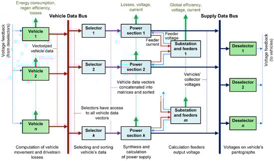
Figure 1.
Proposed structure of the electrified transportation system model.
The vehicle subsystems, acting as transmitters, send their output data vectors to the Vehicle Data Bus, which broadcasts these vectors to receivers. The receivers, which are power section subsystems, use selectors to extract the data of vehicles that run along a particular power section at a considered time. Hence, the selectors perform a task similar to that of frame ID-based filtering used in ICNs. Particular substations are modeled as independent subsystems that exchange data with power section subsystems. This provides the possibility to model various interconnections between the substations and the power sections, and the bilateral influence of their state variables. The power section subsystems send the results of computations to the Supply Data Bus, which broadcasts them to vehicle subsystems. Similarly to the Vehicle Data Bus and the power supply subsystems, the vehicle subsystems use deselectors to extract the results related to particular vehicles. The proposed modeling approach allows for comprehensive analysis of electrified transportation systems, without typical limitations from other solutions. High versatility has been achieved through making the model structure flexible and thanks to local data handling by multiple matrices instead of merging the data into the global matrix.
More details on the data exchange are shown in Figure 2, on the model of a single vehicle and single power section selected as an example. The vehicle subsystem models the vehicle run according to a pre-programmed velocity vs. time profile defined in the look-up table. In order to model the impact of congestion on the trolleybus service, the vehicle subsystem may consist of several velocity profiles (e.g., recorded on the considered route or designed based on the analysis of the route). In such a case, the profiles are selected randomly by a random number generator (RNG) seed assigned to each vehicle. The computations of motion dynamics provide a set of mechanical variables such as motive or braking force, velocity, and covered distance. These computations exchange data with the uploaded route profile, which allows for reflecting additional resistance forces related to riding up or downhill. The vehicle subsection also comprises a look-up table that links the covered distance with the identifier of corresponding power supply section and computes the position of the vehicle within this section.
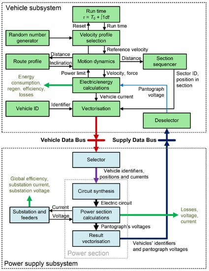
Figure 2.
Data exchange in the model composed of a single vehicle and a single supply section.
The current and energy of the vehicle collector are calculated based on mechanical variables, with consideration of the variable efficiency factor and the current collector voltage. The computed energy is split into consumed, regenerated, and dissipated in the braking resistor. This, along with the drivetrain losses calculation, allows for the complete vehicle energy efficiency analysis. Additionally, a feedback path from electrical-to-mechanical calculations is provided, in order to reflect the power limitation caused by excessively low voltage on the current collector. Each vehicle is represented by an independent subsystem, therefore the number of modeled vehicles may be freely adjusted. Moreover, particular vehicles may have different parameters and may run on different routes.
The vehicle subsystems send the output data vectors to the Vehicle Data Bus. Each of these vectors consists of vehicle identifier kveh, supply section identifier ksec, vehicle collector current iveh, and position of the vehicle in section xveh. The selectors isolate vectors corresponding to particular power sections and store them in local matrices. It is worth noting that the number of vehicles within the section may vary in time, so the local matrix must be declared with respect to the maximum number of vehicles (because variable-size arrays are inefficient or not supported, depending on the programming environment used), and filled with dummy vehicle data in case of a lower vehicle number. The vehicles can run on different routes, and they will not necessarily enter the section always in the same order. Hence, an important role of the selector is to sort the vehicle vectors in the local matrix in order of their location. This is required by the main algorithm of the power section subsystem that merges power section and vehicles data and builds the electric circuit equivalent.
The model of power section synthesizes the electric circuit based on the parameters prepared by the selectors and on the spatial layout and parameters of the power section. The layout of the electric power supply does not change in time, so the data connections between power section subsystems and substation subsystems are fixed. The substation subsystem calculates the feeder output voltage that depends on the load current, internal resistance, and feeder resistance. Since most substations in DC systems are equipped with diode rectifiers, the reverse current is not allowed. Interacting with the linked substations, the power section subsystem calculates the catenary voltage for vehicle nodes (collector voltages) and compiles the data into the result matrices that are delivered to the Supply Data Bus. These matrices consist of vehicle identifiers kveh and current collector voltages uveh. The voltage subsystems use deselectors to extract the collector voltage of particular vehicles. This completes the loop of model computations.
The basic parameters of the analyzed transport network, as well as the initial conditions for the simulation, are loaded from external files. The results are obtained directly from the corresponding models. It is possible to save them into a file or display them as waveforms using commands from outside the simulation.
The models of vehicles, supply sections, and substations are independent—they can be extracted from the main model and used for individual analysis if relevant parameters are provided. The number of vehicles is limited only by the available computer resources, and not by the model design. The modeled vehicles may be of different type and follow individual schedules and routes. Similarly, there is virtually no limit for the number of power sections or connections between them. This allows for simulating complex transport networks because the sectors need only be connected with the data buses and the substation, while the connection between them is defined in the initial parameters file. Since the power sections also have their identifiers and localization parameters, the implementation of branches can be achieved easily—the power section can be connected in the same manner as the vehicles (but with constant location).
Using Simulink as the programming environment has some limitations. The most notable one is the lack of dynamic matrix size. Moreover, the input and output ports of the program blocks have fixed width [31]. To deal with these limitations, countermeasures in the form of data buses, selectors, and deselectors were implemented. It is also worth noting that all variables in the matrices must be of uniform numeric type. The program is designed to use the ode3 solver and a fixed time step equal to 1 s, which provides sufficient accuracy while retaining high computing performance [32]. The selection of time step has been validated by comparing simulation results obtained for execution with the chosen and decreased time step (0.01 s). For the simulation of a 10-min trolleybus run, the difference in its consumed energy was less than 0.5%. The time-step size of 1 s has been commonly used also in similar models [3,6,8,18].
3. Vehicle Subsystem
Each modeled vehicle has its individual subsystem that includes vehicle parameters, timetable, route inclination profile, and reference speed profiles. The ability to follow the reference speed profile is constrained by several factors of both mechanical and electrical nature. The vehicle motion is modeled mostly using kinematic equations, but the vehicle subsystem also includes algorithms that compute losses of conversion between electric and mechanical power. Some control-related factors are also included, e.g., the power limitation due to excessive voltage drop at the current collector.
3.1. Reference Speed Profiles and Timetabling
The reference speed profiles must be prepared before the execution of the model and stored in the look-up tables that are uploaded to the vehicle subsystem. Trolleybuses run along public roads, so modeling their ride with simple velocity profiles that include a sequence of acceleration, cruising, coasting, and braking would not reliably reflect their complex operating conditions. Therefore, the reference velocity profiles for the analyzed case were prepared with the use of onboard vehicle data recorders. For each considered trolleybus line and each type of vehicle, numerous recordings were carried out to obtain a representative set of reference velocity profiles. The recordings include runs that took place at different times of the day, in order to reflect time-specific factors such as traffic, stop-at-lights patterns, etc. This allows for aligning the recorded runs into groups representing morning rush, midday, afternoon rush, and evening operation. The recordings also include dwelling time, so analysis of their content allows for the determination of minimal and maximal times that the trolleybuses spent at particular stops.
The aim of the proposed model is to reflect both deterministic features of the transportation system, such as the operation according to the timetable, and stochastic features such as different run and dwelling times. This is achieved by a set of signals that control the time when the vehicle enters the modeled area of the transportation system and when it starts the run from the terminal (end stop). These signals are also used for the random selection of velocity profiles related to rides between stops (featured by different run times) as well as the random selection of dwelling times at stops.
Exemplary waveforms of vehicle control signals are presented in Figure 3. The permission signal, when active, allows for the run of a given vehicle. The rising slope of this signal determines the time when the vehicle enters the considered area of the transportation system or resumes the operation after a service pause at the end stop (terminal). Each run between stops is initiated by the triggering signal, whose impulses are counted by the run counter. The initial value of this counter must be set before model execution to define the initial position of the vehicle. The value of the run counter determines between which stops the trolleybus is running. Each run starts with selecting the reference velocity profile from the set related to the considered route, stored in the vehicle subsystem. This selection is based on the random number generator (RNG). The probability of selecting each profile recorded for a considered route between stops is not equal. The RNG uses global simulation time to set weights for selecting profiles related to the different parts of the day. The highest probability is attributed to the group of velocity profiles that were recorded in the time similar to the actual global simulation time. The RNG is also used to set the dwelling time at the next stop (not shown in Figure 3). In this process, the range of selected numbers is defined by minimal and maximal time derived based on the recordings.
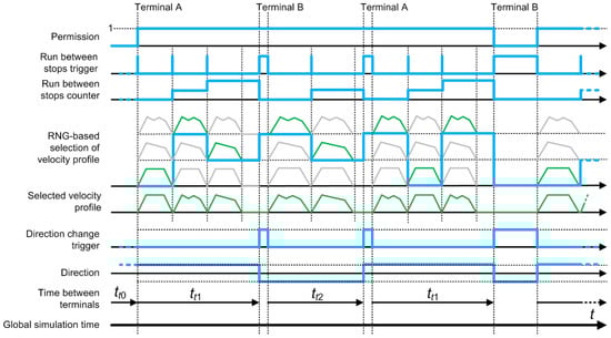
Figure 3.
Control signals used in vehicle subsystem.
The reference velocity profiles feature slightly different times of travelling between stops. As these times, as well as dwelling times at stops, are selected randomly, the travelling time between terminals (end stops) may vary. Hence, the maximal time for travelling between the terminals must be assumed, and if the vehicle reaches the end stop sooner than this time expires, the time that it spends at this stop is prolonged according to the recorded difference. This travelling time is reflected by the direction change signal, whose rising slope represents the latest assumed arrival at the end stop, while the falling slope determines the departure. The rising slope in the direction change signal also reverses the value of the direction signal, which can be set to −1 or 1. The value of the direction signal is multiplied by velocity in the algorithm computing the vehicle motion dynamics. This, in turn, influences the computations of the covered distance, which increases or decreases depending on the direction of movement.
3.2. Vehicle Motion Dynamics
The vehicle can be considered as a material point (vehicle mass is concentrated at a single point), which greatly reduces the complexity of the model. This assumption provides satisfactory modeling accuracy for most types of vehicles, except for freight trains with a large number of wagons, where the mass is distributed along a distance of hundreds of meters [33].
The equation for vehicle dynamics is given by:
where a is the vehicle acceleration, F is the total motive force, W is the resistance force, m is the vehicle mass, and k is the coefficient of rotating mass.
By integrating the result of (1), the model computes the vehicle speed. Then, double integration provides the covered distance. In (1), the vehicle mass m is increased artificially by multiplying it by the coefficient k, whose value is slightly greater than 1 (for trolleybuses: k = 1.2 [34]). This mass increase reflects the impact of the moment of inertia of drivetrain rotating parts on the vehicle acceleration.
The total motive force F is either propelling (positive) or braking (negative), and its value is controlled by the driver. The positive motive force is generated solely by the electric drive. Hence, its value is limited by the nominal power and torque of the drive, see further comments in Section 3.3. The negative motive force that occurs during braking may be generated by both electric drive and friction brakes. The distribution of the braking force (set by the driver) between the electric drive and the friction brakes is performed by the drivetrain control algorithm.
The motion resistance W is the sum of resistance forces that can be attributed to the vehicle (fundamental resistance Wf) and the route (additional resistance Wi). The fundamental motion resistance of the vehicle is calculated as the sum of aerodynamic drag, transmission drag, and rolling resistance. The following second-order polynomial is used to approximate the value of the fundamental resistance force:
where v—the vehicle velocity; A, B, C—the coefficients of the fitting function (e.g., for Škoda 26Tr trolleybus: A = 1175.82 N, B = 0 N/(m/s), C = 3.71 N/(m/s)2).
The additional motion resistance Wi, related to route inclination, is calculated as:
where g is the gravitational acceleration and i is the longitudinal inclination of the route.
The route profile that defines the route inclination as a function of covered distance can be derived from GPS recordings or extracted from a map supported by Shuttle Radar Topography Mission (SRTM)-based altitude data.
3.3. Control of Motive Force
The vehicle subsystem is designed to regulate the motive force F in such a way as to follow the reference velocity profile. This is carried out by the use of the proportional-integral (PI) controller that sets the value of total motive force F according to the error computed as the difference between reference and actual speed of the vehicle (Figure 4). The gains for the proportional and integral terms were tuned to ensure control dynamics similar to those observed during the experiments. Since the controller output depends on the velocity error and its gains, the resulting force value can exceed the maximum motive force available in the traction drive. This cause of possible errors was solved by saturating the PI controller output (value of motive force) with respect to factors described below.
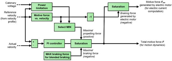
Figure 4.
Structure of the algorithm computing motive force of the vehicle.
The maximal output torque of an electric drive (hence also the motive force) is most commonly defined as a function of velocity (see Figure 5). Upon low velocities, the maximal output torque is constant. However, after reaching the base speed at which the nominal value of output power is achieved, the torque is limited according to the constant (nominal) power curve. In certain operating conditions, the available motive force may be further decreased. For instance, if the voltage on the trolleybus current collector drops below a predefined value, the output power of the electric drive is decreased linearly with respect to the catenary voltage in order to prevent further voltage drop and to sustain the stability of the supply system. Such emergency power limitation was implemented into the model [35]. When modeling some transportation systems (e.g., railway), it is sometimes desired to reflect limited adhesion of driving wheels [36]. However, in the trolleybus system, it is assumed that wheel slip or skid do not occur. The above-mentioned limitations of the propelling force generated by the electric drive were implemented as the upper saturation threshold for PI controller output (see Figure 4).
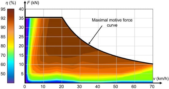
Figure 5.
Efficiency map of a 200-kW trolleybus induction motor.
The negative motive force, which corresponds to braking, was assumed as a blended force generated by friction brakes and electric drive. The latter part used for braking is commonly referred to as an electrodynamic brake. The available braking force related to blended braking has large values, allowing even for emergency braking, but this is assumed not to occur in the simulated case. However, for formal reasons, the maximal braking force was defined and used to set the lower saturation threshold for the PI controller output (see Figure 4). This value is negative as it corresponds to braking.
To compute the vehicle dynamics (1) for the braking regime, the total motive force F generated by both electrodynamic and friction brakes should be considered. However, the vehicle subsystem also includes computations related to the electric drive. For these computations, it is necessary to isolate the braking force Fem generated solely by the electric motor. In most blended braking systems, the vehicle controller maximizes the use of electrodynamic brake to save friction brake pads and allow for generating the electric power that can be delivered to other vehicles. Therefore, it was assumed that friction brakes are engaged only if the total braking force exceeds the value defined by the electric drive relation between the motive force and velocity (Figure 5). Consequently, the motive force generated by the electric drive is computed as a total motive force with a lower saturation threshold set accordingly to the inverted (negative) maximal electric drive motive force at actual speed.
3.4. Electric Drive Efficiency and Electric Current Computation
Electric current Iveh collected by the vehicle is determined from mechanical power on electric drive output but also includes other important factors. The electric current is computed from the following formula:
where (Fem·v) is the mechanical power on electric motor output (may be either positive or negative); Pbr_res is the power dissipated in the braking resistor (positive or zero); Paux is the power of auxiliary loads (positive); Pmech_loss, Pem_loss, Pinv_loss, are the power losses in electric motor, power inverter, and the mechanical part of the drivetrain, respectively (positive or zero); and Uveh is the voltage on vehicle pantograph.
In order to exclude the operation of friction brakes, which has no impact on the vehicle current, the mechanical power computed using Equation (4) is not based on total motive force F but the part of this force Fem generated by the electric motor.
The power balance in the numerator of (4) includes power Pbr_res dissipated into the heat in the vehicle braking resistor. This power is equal to zero during propelling and coasting. On the other hand, Pbr_res may be positive during braking if other vehicles on the same power supply section are unable to consume the electric power generated by regenerative braking in the considered vehicle. The power Pbr_res is controlled using the vehicle pantograph voltage Uveh and voltage threshold levels. Typically, the braking resistor is engaged when the pantograph voltage exceeds 760 V. The power Pbr_res increases linearly with the further rise of Uveh, reaching the full value of vehicle power balance at Uveh = 790 V. Conversely, when the vehicle pantograph voltage falls below 580 V, the vehicle power is reduced linearly down to zero at Uveh = 520 V, which is the minimum allowed voltage for traction drive of the analyzed vehicle.
The auxiliary power was set at a constant value, Paux = 2.5 kW, derived from onboard recordings carried out in trolleybuses during their standstill. In the period when the recordings were carried out, heating and air conditioning were not used.
The efficiency of the mechanical part of the drivetrain was set at 95%. It was assumed that there is no need to model the variable efficiency, as the operating conditions related to significant efficiency drops (very low torque or speed) do not occur often during trolleybus runs [37].
Computing power losses Pem_loss in the electric motor and Pinv_loss in the power electronic inverter is a complex problem. As the operating conditions of vehicle drives change in a wide range, assuming a constant efficiency would lead to considerable errors [38]. Trolleybuses in the considered transportation system use induction motor drive. The induction motor converts electric to mechanical power using the electromagnetic field. The efficiency of the induction motor is highly dependent on angular velocity and torque. While for most operating conditions the efficiency exceeds 90%, there are also low-efficiency regions corresponding to the low-speed and low-load operation. In order to accurately reflect motor power losses in the model, the efficiency map η = f(T,ω) is required. Since experimentally derived efficiency values were unavailable, the authors used parameters of the electric motor to set up a mathematical model, which was used to compute losses as a function of velocity and torque. The obtained dataset was loaded into the vehicle subsystem as a 2-dimensional lookup table, where the efficiency values for arguments between the defined points are computed using linear interpolation. A graphical representation of the derived efficiency map is shown in Figure 5.
A detailed analysis of the power electronic inverter would require simulating transient states related to the switching of its transistors. This, in turn, would lead to setting simulation time step at the order of microseconds, which is unjustified for other parts of the considered model. Therefore, the inverter losses are estimated based on the actual operating conditions and parameters of power electronic components specified in their datasheets. The total inverter losses Pinv_loss are computed as the sum of switching losses of transistors Pt_sw, reverse-recovery diode losses Pd_rec, and conduction losses for both diodes Pd_cond and transistors Pt_cond [39,40]. All these losses need to be included because the typical voltage drop of 1.2–2.5 V on a semiconductor switch translates to kilowatts of losses.
A typical traction power inverter consists of 6 transistors and 6 freewheeling diodes, so the total power losses in the inverter can be approximated as:
For a single transistor, the switching losses are approximated as [39,40]:
where Uveh_n—the nominal voltage at vehicle collector (on inverter DC bus); Esw_on and Esw_off—energy losses for switching the transistor on and off, respectively; f—the switching frequency.
The reverse recovery losses of a diode are calculated as [39]:
where Erec—energy dissipated due to the reverse recovery charge current.
The conduction losses for a transistor and a freewheeling diode are computed according to (8) and (9), respectively [38,39]:
where IC—collector current; UCE—collector-emitter saturation voltage; D—inverter duty cycle; cos—power factor of the motor; and Uf—diode forward voltage drop.
The collector current IC of the transistor and diode was assumed equal to the vehicle motor current Iveh—averaged over the duty cycle. The motor power factor was implemented in the second term of Equations (8) and (9).
4. Power Supply Subsystem
The power supply of electrified transportation systems may have a complex structure, especially in the case of an urban system. The trolleybus supply system consists of traction substations that transform the electric power from medium-voltage AC to DC voltage at a level of 600–700 V, which is suitable for vehicles. Typically, a trolleybus traction substation has a rated power of a few hundred kilowatts and supplies the catenary at the area of several square kilometers. The catenary is divided into power sections of a typical length of a few hundred meters. The substation supplies several neighboring power sections through separate feeders (supplying cables). The neighboring power sections of the catenary are electrically separated from each other by section insulators fixed to the catenary. However, they are electrically linked by the feeders if they are supplied from the same substation. Some power sections may include intersections and then the catenary has some side branches. Unlike railways, power sections of urban systems are supplied from a single traction substation. However, several feeders may connect the substation to different points of the power section.
The power supply subsystem includes models of power sections and traction substations. Such a model composition allows for flexible representation of complex supply structures. Moreover, such a division splits the process of numerical solving into smaller portions, which is favorable in terms of computation performance and stability. Following the above-discussed features of the trolleybus supply system, typically a single substation model is linked to models of several associated power sections.
4.1. Traction Substation and Feeders
The model of substation and feeders computes the output voltages for the feeders. The results are delivered to the linked power section model. The traction substation is modeled as voltage source E and internal series resistance Rs. Such a model reflects the voltage drop at substation output (at its DC switchgear) that is linear to the output current. The best method to derive the model parameters is to analyze the recordings collected during the operation of the considered substation. Approximating the relation between the substation output voltage Usub and output current Isub with a linear function allows for deriving both the idle voltage E (as the voltage for Isub = 0) and the series resistance (as the slope coefficient of the linear function).
The traction substation model is supplemented by the models of all feeders associated with this substation. The feeders are modeled as series resistances Rfdr whose values depend on the feeder length, cross-section, and the restiveness of the material used (typically aluminum). The trolleybus catenary is symmetrical, i.e., the feeders and the catenary contact wires are identical for positive and negative poles. For simplicity, each feeder is modeled as a single resistance Rfdr, whose value is the sum of resistances of both negative and positive pole feeders. The feeders of the substation have different lengths and different load currents, so the output voltage for each feeder needs to be computed individually. The output voltage for the k-th feeder in the substation supplying n feeders is computed as follows:
The resistances of the feeders are also used for computing the power transmission losses in the feeders:
The substations in the DC supply systems are usually equipped with diode rectifiers, so they do not allow reverse current. To reflect this property, the value of the modeled internal resistance Rs is a function of the substation output current Isub. The resistance Rs increases when the output current approaches zero and saturates at 1 GΩ for negative currents. Such a continuous change of resistance synergizes well with the voltage-dependent reduction of regenerative braking power implemented in the vehicle model and ensures stable operation of the numeric solver.
4.2. Power Section
The power section model uses a circuit equivalent of the catenary to compute feeder currents and voltages at vehicle pantographs. The feeders are modeled as voltage sources with values obtained from the model of substation and feeders. The vehicles are modeled as current sources, whose values are set according to the vehicle data obtained from the Vehicle Data Bus through the selector (see Figure 1). The catenary is modeled as series resistance Rcat. The catenary is assumed to have a unified value of unit resistance Rcat′ expressed in Ω/m. Consequently, the resistances between the mentioned current and voltage sources are computed based on their distances. The layout of the catenary is fixed, which also refers to the positions where the feeders are connected to the catenary. The variable topology of the equivalent circuit is related to the number and positions of vehicles that run within the considered power section. This problem is resolved by assuming a maximal number of vehicles in the equivalent circuit. If the actual number of vehicles is lower, the current sources related to absent vehicles are set to zero (while their set positions may be arbitrary). Consequently, the absent vehicles do not influence the current distribution in the circuit. This approach leads to a fixed structure of the equivalent circuit, where the values of voltage sources, current sources, and resistances are not stationary. Such a circuit can be solved with relatively simple and fast methods.
Another means that simplifies the equivalent circuit synthesis is sorting the vehicles related to the considered power section according to their position, which is done by the selector. Due to the sorting, it is easy to automatically set the catenary resistances and current source values according to the received data at each step of numeric computations.
Typical structures of power sections and their equivalent circuits are shown in Figure 6.
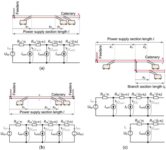
Figure 6.
Typical structures of power sections and their equivalent circuits: (a) power section supplied by one set of feeders connected at the boundary; (b) power section supplied by two sets of feeders at boundaries; (c) power section supplied by one set of feeders with a branch in the middle part.
The most common case of power supply section layout is shown in Figure 6a, where a single set of feeders is connected at the boundary of the power section. This case can be solved using self-reliant mathematical formulas for each derived parameter. A much less frequent case, where the power section is supplied by two sets of feeders is presented in Figure 6b. In this case, both feeders are supplied from the same substation. However, due to their different length and load, the output voltages of the feeders (represented by voltage sources Ufdr1 and Ufdr2) are different. This case can be solved automatically, e.g., by nodal analysis, which leads to solving the following set of equations:
If there are two or more sets of feeders connected to the power section, but not at the boundaries (the case not shown in Figure 6), such a section can be modeled as a combination of several self-reliant circuits from the set shown in Figure 6a,b.
Figure 6c shows a more complex case, where a part of supply sections splits into two branches. The side branch of the catenary may be considered as a subcircuit represented by a current source whose value is equal to the total current of the vehicles running at the branch.
Since all vehicle models communicate with the power supply model using the Vehicle Data Bus (see Figure 1), there is no explicit limitation to the system layout. When part of the power section branches off, this case can be implemented as a separate stationary section in the place where it is connected to the main line.
The output values calculated by the power section model are loaded into the data vectors along with the corresponding vehicle ID—the order of results is consistent with that of vehicles. This allows omitting the use of search functions or multidimensional matrices, thus improving the simulation performance. The data vectors are then sent to the Supply Data Bus, where they are awaited by the deselectors, which send the line voltage value to individual vehicles.
Aside from the above-discussed results, the power section model computes the power transfer losses related to the catenary. This is done in a similar manner to computing power transfer losses in feeders (11).
5. Experimental Verification
The proposed model was verified within the framework of the Interreg project “EfficienCE”, where the improvement of energy efficiency in urban electrified transportation is the main objective. The model was parametrized according to a part of the trolleybus network in the City of Pilsen, Czech Republic.
The Pilsen supply system for electrified transportation systems includes 10 traction substations that supply both trolleybuses and trams. The verification was carried out for the supply area of substation MR5 (Figure 7), which was selected because all vehicles running in this area are equipped with AC-motor drive that enables regenerative braking. The verification covered a single workday operation (from 4 a.m. to midnight).
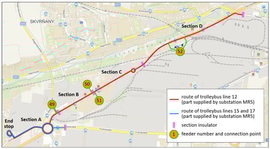
Figure 7.
Topography of trolleybus power supply area supplied by substation MR5 in Pilsen.
The substation MR5 supplies both trolleybus and tram supply sections. The verification was focused on the trolleybus system, but the trams have a notable influence on the operation of the substation and the trolleybus supply section voltages. Therefore, in order to include this influence, the load caused to the substation by the trams was recorded during a selected mid-week day and this recording was used to set current waveforms of the tram feeders in the model. The trolleybus supply sections powered from substation MR5 are shown in Figure 7.
The substation MR5 powers four trolleybus supply sections (marked from “A” to “D” in Figure 7) and three tram supply sections (not included in Figure 7). Two of the trolleybus sections are supplied by feeders connected at the boundaries, i.e., sections B and C. These sections are represented by the equivalent circuit shown in Figure 6a. Section D is supplied by two sets of feeders marked as 52A and 52B, and these sets are connected to the catenary at a 230-m distance. This section is represented by a set of equivalent circuits composed of one circuit shown in Figure 6b and two circuits from Figure 6a. The south section, marked as A, is powered by twin feeders connected to the catenary at the same point. Hence, they may be modeled as a single set of feeders with a double cross-section. However, this section includes a branch that leads to the Nova Hospodá loop, which is the end stop for trolleybuses. This branch is represented in the model as the equivalent circuit shown in Figure 6c.
The area lies within the bounds of trolleybus lines 12, 15, and 17 (as well as tram line 2). The locations of the trolleybus stops and the route lengths are shown in Figure 8. The trolleybuses on lines 15 and 17 enter section A from the east (Folmavska Rondel stop), and then move west to the end stop Nova Hospodá and backward. At the same time, the trolleybuses on line 12 enter the supply section D from north-east (Škoda III. brána stop) and then ride to the end stop Nova Hospodá and backward.
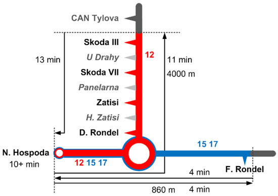
Figure 8.
Trolleybus lines and stops in the supply area of substation MR5 (on-request stops are marked in grey).
Lines 12 and 15 are operated by standard two-axle trolleybuses type 26Tr. Line 17 is serviced by three-axle articulated vehicles type 27Tr. The parameters of these vehicles were provided by the manufacturer, Škoda Electric. The most important parameters used for the simulation are specified in Table 1.

Table 1.
Parameters of modeled trolleybuses.
The model was set up according to a workday timetable. The schedule for line 12 begins with a 15-min service interval between subsequent runs, which is decreased to 5 min during the morning peak hours, i.e., between 5 a.m. and 8 a.m. Then, between 8 a.m. and 1 p.m., this interval is increased to 10 min. From 1 p.m. to 3 p.m., there is another peak with a 5-min interval, which from 5 p.m. starts increasing gradually to 10 min. The service interval is further increased to 15 min in the evening, starting from 7 p.m. Trolleybuses on line 15 operate with a 30-min service interval during the whole day, starting from 5:12 a.m. Vehicles on line 17 run along the analyzed area regularly between 5:20 and 6:00 a.m., with a 5-min interval. During the rest of the day, trolleybuses on line 17 appear at the analyzed area rarely, during only a few services.
The maximal number of vehicles running simultaneously in each supply section is 6 for section A and 4 for each of the sections B, C, and D. These values were used to set the number of vehicle nodes in the equivalent electrical circuits included in the power supply section models.
The model was verified by comparing the simulation outcomes with real measurements from substation MR5 in Pilsen. The time of the measurements was the same as in simulation, i.e., workday from 4 a.m. until midnight. The collected measurements cover the voltage at the substation output bars and the currents of the substation feeders.
The currents and voltages, both in the measurements and simulation, were post-processed to obtain the following quantities that were used for verification:
- substation total output current: sum of feeder currents in substation MR5;
- substation output voltage: voltage at substation MR5 output bars; and
- substation output energy: integral of the total output power of substation MR5.
The model executes according to the timetable. As, in fact, the real operation times of the trolleybuses differ slightly from the scheduled time, the instantaneous voltage, current, and power values may differ between the model and the measurements. In order to disregard these differences, the waveforms of substation output voltage and current were averaged using a standard 15-min averaging window. The averaged variables still reflect daily load changes due to varying frequency of services well. The output energy does not require averaging as its computation involves integration.
The results of the verification are shown in Figure 9, Figure 10 and Figure 11. Figure 9 compares the 15-min averages of substation output current. The results show good conformance between the measurement and simulation, considering the variability of the trolleybus network. The greatest current values were observed during morning peak hours when the service frequency was the highest. The current differences between 5 a.m. and 7:30 a.m. can be attributed to the differences between the assumed and the actual heating power and vehicle mass, which was set constant in the simulation. During the evening hours, the simulated current values slightly exceeded the measured ones, most likely due to traffic conditions and differences in the number of carried passengers.
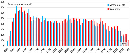
Figure 9.
Verification results: substation total output current (15-min average).
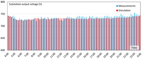
Figure 10.
Verification results: substation output voltage (15-min average).
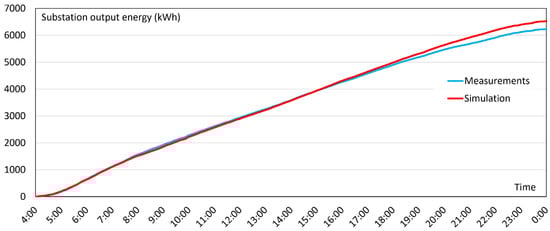
Figure 11.
Verification results: substation output energy.
Figure 10 shows the 15-min averages of substation output voltage. The voltage values were very similar for both the measurement and simulation, with only small differences reflecting the deviations in substation output current that were commented in the previous paragraph. The 15-min averages of current (Figure 9) showed good agreement between the measurement and simulation, and the 15-min averages of voltage (Figure 10) were almost exactly equal. This confirms the good accuracy of the proposed model and therefore, the good feasibility of the simulation results.
In order to quantify the differences between measured and simulated waveforms of substation current and voltage, Root Mean Square Errors (RMSEs) were computed. The RMSE for the output voltage was 8.8 V, which constitutes less than 2% of the idle-state voltage. The RMSE for the output current was 49.2 A, i.e., 7% of the maximal measured current.
Figure 11 compares the output energy waveforms. Both waveforms are rising monotonously, as no energy can be delivered back to the substation. The end value of the energy obtained in the simulation was relatively close to that computed from the measurements. The notable and increasing difference between the waveforms was observed in the evening. The obtained results are consistent with the values of current and voltage. The observed differences stem from the assumed input parameters and the set schedule. As the deviation was less than 4.5%, the differences are within the expected margin.
The performed verification has shown that good conformance between the measurement and the simulation was achieved. Slight differences can be attributed to unavailable parameters, which could not be set accurately in the model. For instance, the number of passengers was set constant in the simulation, whereas the real number varies in different services. Moreover, accurate modeling of auxiliary loads, such as heating and air conditioning, would require an additional thermal analysis [41] and precise knowledge about the weather and vehicle climate control settings. This knowledge was not available. Finally, the variability of traffic congestion was dealt with in the simulation by randomly selecting the recorded velocity profiles. However, the traffic conditions on particular days may differ due to specific occurrences.
6. Conclusions
The proposed model includes both mechanical and electrical subsystems of a transportation system, which makes it a comprehensive and versatile tool for various analyses. Adopting a structure similar to the industrial communication networks enables local data processing within the subsystems and overcomes common restrictions found in similar models. The verification carried out for an exemplary trolleybus system showed good accuracy of the model. Both the error in total energy consumption (less than 5%) and the RMSEs of substation current and voltage (7% and 2%, respectively) are considered satisfactorily small, taking into account numerous factors that could not be precisely reflected. The errors would have probably been even lower if the variable number of passengers and the variable auxiliary power were considered in the model. The model is ready for such a parametrization, but the mentioned factors were unknown in the analyzed case.
The model may be used for analyzing the behavior of both vehicles and power supply working under realistic operating conditions. The implementation of RNG-based velocity profile selection improves the accuracy of modeling variable traffic conditions. The use of Matlab as the programming basis allows for model interaction with numerous toolboxes and scripts. This, in turn, enables multi-objective optimization that is not limited by any program code and is compatible with other works carried out in this environment.
In future work, the authors are going to use this model to seek the optimal idle voltage of substations. Increasing the idle voltage minimizes the transmission losses but decreases the utilization of regenerative braking energy. The presented model will help to find the optimal value of the idle voltage in terms of total energy consumption.
The authors also plan to use this model for analysis focused on the behavior of trolleybuses equipped with onboard battery storage and the impact of these vehicles on the supply system. The model is suitable for including the battery-assisted vehicles, and authors expect to receive experimental recordings, which will be used to set and validate the model.
Author Contributions
Conceptualization, M.B. and L.J.; methodology, A.J. and L.J.; software, A.J.; validation, A.J. and M.P.; formal analysis, S.J.; resources, J.S.; writing—original draft preparation, A.J.; writing—review and editing, L.J.; visualization, A.J. and L.J.; supervision, S.J., J.S. and A.W.; project administration, M.B. and A.W.; funding acquisition, M.B. All authors have read and agreed to the published version of the manuscript.
Funding
This research was funded by Interreg CENTRAL EUROPE, within the framework of the grant agreement no CE1537, project title “EffcienCE—Energy Efficiency for Public Transport Infrastructure in Central Europe”.
Acknowledgments
The authors would like to thank Plzeňské Městské Dopravní Podniky A.S. (PMDP) for sharing results of recordings that were used for verification of the developed model.
Conflicts of Interest
The authors declare no conflict of interest.
References
- Radtke, A.; Muller, L.; Schumacher, A. DYNAMIS: A model for the calculation of running times for an efficient time-table construction. Trans. Built Environ. 1998, 34, 309–317. [Google Scholar] [CrossRef]
- TranSys Research Ltd.; RailTEC at the University of Illinois at Urbana-Champaign; CPCS Transcom; Lawson Economics Research Inc.; National Cooperative Railroad Research Program; Transportation Research Board; National Academies of Sciences, Engineering, and Medicine. Comparison of Passenger Rail Energy Consumption with Competing Modes; Transportation Research Board: Washington, DC, USA, 2015; p. 22083. [Google Scholar] [CrossRef]
- Caramia, P.; Mottola, F.; Natale, P.; Pagano, M. Energy Saving Approach for Optimizing Speed Profiles in Metro Application. In Proceedings of the 2016 International Conference on Electrical Systems for Aircraft, Railway, Ship Propulsion and Road Vehicles & International Transportation Electrification Conference (ESARS-ITEC), Toulouse, France, 2–4 November 2016; pp. 1–5. [Google Scholar] [CrossRef]
- Alnuman, H.; Gladwin, D.; Foster, M. Electrical Modelling of a DC Railway System with Multiple Trains. Energies 2018, 11, 3211. [Google Scholar] [CrossRef]
- Douglas, H.; Roberts, C.; Hillmansen, S.; Schmid, F. An Assessment of Available Measures to Reduce Traction Energy Use in Railway Networks. Energy Convers. Manag. 2015, 106, 1149–1165. [Google Scholar] [CrossRef]
- Tian, Z.; Hillmansen, S.; Roberts, C.; Weston, P.; Zhao, N.; Chen, L.; Chen, M. Energy Evaluation of the Power Network of a DC Railway System with Regenerating Trains. IET Electr. Syst. Transp. 2016, 6, 41–49. [Google Scholar] [CrossRef]
- Açikbaş, S.; Söylemez, M.T. Parameters Affecting Braking Energy Recuperation Rate in DC Rail Transit. In Proceedings of the ASME/IEEE 2007 Joint Rail Conference and Internal Combustion Engine Division Spring Technical Conference, Pueblo, CO, USA, 13–16 March 2007; pp. 263–268. [Google Scholar] [CrossRef]
- Tian, Z.; Zhang, G.; Zhao, N.; Hillmansen, S.; Tricoli, P.; Roberts, C. Energy Evaluation for DC Railway Systems with Inverting Substations. In Proceedings of the 2018 IEEE International Conference on Electrical Systems for Aircraft, Railway, Ship Propulsion and Road Vehicles & International Transportation Electrification Conference (ESARS-ITEC), Nottingham, UK, 7–9 November 2018. [Google Scholar] [CrossRef]
- Koseki, T. Technologies for Saving Energy in Railway Operation: General Discussion on Energy Issues Concerning Railway Technology. IEEJ Trans. Electr. Electron. Eng. 2010, 5, 285–290. [Google Scholar] [CrossRef]
- Sanchis, I.V.; Zuriaga, P.S. An Energy-Efficient Metro Speed Profiles for Energy Savings: Application to the Valencia Metro. Transp. Res. Procedia 2016, 18, 226–233. [Google Scholar] [CrossRef]
- Xiao, Z.; Wang, Q.; Sun, P.; You, B.; Feng, X. Modeling and Energy-Optimal Control for High-Speed Trains. IEEE Trans. Transp. Electrif. 2020, 6, 797–807. [Google Scholar] [CrossRef]
- Bosyi, D.; Kosariev, Y. Modeling of the controlled traction power supply system in the space-time coordinates. Transp. Probl. 2017, 12, 5–19. [Google Scholar] [CrossRef]
- Frilli, A.; Meli, E.; Nocciolini, D.; Pugi, L.; Rindi, A. Energetic Optimization of Regenerative Braking for High Speed Railway Systems. Energy Convers. Manag. 2016, 129, 200–215. [Google Scholar] [CrossRef]
- Tian, Z.; Hillmansen, S.; Roberts, C.; Weston, P.; Chen, L.; Zhao, N.; Su, S.; Xin, T. Modeling and Simulation of DC Rail Traction Systems for Energy Saving. In Proceedings of the 17th International IEEE Conference on Intelligent Transportation Systems (ITSC), Qingdao, China, 8–11 October 2014; pp. 2354–2359. [Google Scholar] [CrossRef]
- Krzysztoszek, K. Mathematical Model of Traction Vehicle Movement. J. Autom. Electron. Electr. Eng. 2019, 1, 37–42. [Google Scholar] [CrossRef][Green Version]
- Krzysztoszek, K.; Luft, M.; Lukasik, Z. Digital Control Model for Electric Traction Vehicles. Procedia Comput. Sci. 2019, 149, 274–277. [Google Scholar] [CrossRef]
- Train Energy and Dynamics Simulator (TEDS). U.S. Department of Transportation, Federal Railroad Administration. Available online: https://railroads.dot.gov/rolling-stock/current-projects/train-energy-and-dynamics-simulator-teds (accessed on 30 May 2021).
- OpenPowerNet Simulation Software for Traction Power Supply Systems. Institut fuer Bahntechnik GmbH. Available online: https://www.openpowernet.de (accessed on 15 May 2021).
- Dynamis. IVE mbH—Ingenieurgesellschaft für Verkehrs-und Eisenbahnwesen mbH. Available online: https://www.ivembh.de/softwareprodukte/simulation/dynamis.html (accessed on 25 June 2021).
- Matsuoka, K.; Kondo, M. Energy Saving Technologies for Railway Traction Motors. IEEJ Trans. Electr. Electron. Eng. 2010, 5, 278–284. [Google Scholar] [CrossRef]
- Torreglosa, J.P.; Garcia, P.; Fernandez, L.M.; Jurado, F. Predictive Control for the Energy Management of a Fuel-Cell–Battery–Supercapacitor Tramway. IEEE Trans. Ind. Inform. 2014, 10, 276–285. [Google Scholar] [CrossRef]
- Zarifian, A.; Kolpahchyan, P.; Pshihopov, V.; Medvedev, M.; Grebennikov, N.; Zak, V. Evaluation of electric traction’s energy efficiency by computer simulation. In Proceedings of the 2013 19th IMACS World Congress, San Lorenzo del Escorial, Spain, 26–30 August 2013. [Google Scholar]
- Du, F.; He, J.H.; Yu, L.; Li, M.X.; Bo, Z.Q.; Klimek, A. Modeling and Simulation of Metro DC Traction System with Different Motor Driven Trains. In Proceedings of the 2010 Asia-Pacific Power and Energy Engineering Conference, Chengdu, China, 28–31 March 2010; pp. 1–4. [Google Scholar] [CrossRef]
- Fathy Abouzeid, A.; Guerrero, J.M.; Endemaño, A.; Muniategui, I.; Ortega, D.; Larrazabal, I.; Briz, F. Control Strategies for Induction Motors in Railway Traction Applications. Energies 2020, 13, 700. [Google Scholar] [CrossRef]
- Apostolidou, N.; Papanikolaou, N. Energy Saving Estimation of Athens Trolleybuses Considering Regenerative Braking and Improved Control Scheme. Resources 2018, 7, 43. [Google Scholar] [CrossRef]
- Tian, Z.; Zhao, N.; Hillmansen, S.; Su, S.; Wen, C. Traction Power Substation Load Analysis with Various Train Operating Styles and Substation Fault Modes. Energies 2020, 13, 2788. [Google Scholar] [CrossRef]
- Du, G.; Wang, C.; Liu, J.; Li, G.; Zhang, D. Effect of Over Zone Feeding on Rail Potential and Stray Current in DC Mass Transit System. Math. Probl. Eng. 2016, 2016, 1–15. [Google Scholar] [CrossRef]
- Baumeister, D.; Salih, M.; Wazifehdust, M.; Steinbusch, P.; Zdrallek, M.; Mour, S.; Lenuweit, L.; Deskovic, P.; Ben Zid, H. Modelling and simulation of a public transport system with battery-trolleybuses for an efficient e-mobility integration. In Proceedings of the 2017 1st E-Mobility Power System Integration Symposium, Berlin, Germany, 23 October 2017. [Google Scholar]
- He, X.; Li, E.; Zhang, H. ASR Control of Distributed Drive Vehicles Based on CAN Bus and FlexRay Bus. In Proceedings of the 2021 IEEE 5th Advanced Information Technology, Electronic and Automation Control Conference (IAEAC), Chongqing, China, 12–14 March 2021; IEEE: Piscataway, NJ, USA; pp. 749–755. [Google Scholar] [CrossRef]
- Murvay, P.-S.; Groza, B. Efficient Physical Layer Key Agreement for FlexRay Networks. IEEE Trans. Veh. Technol. 2020, 69, 9767–9780. [Google Scholar] [CrossRef]
- MathWorks Inc. Matlab Programming Fundamentals. Available online: https://www.mathworks.com/help/pdf_doc/matlab/matlab_prog.pdf (accessed on 11 April 2021).
- Shampine, L.F.; Reichelt, M.W. The MATLAB ODE Suite. SIAM J. Sci. Comput. 1997, 18, 1–22. [Google Scholar] [CrossRef]
- Muginshtein, L.A.; Yabko, I.A. Power Optimal Traction Calculation for Operation of Trains of Increased Mass and Length. In Proceedings of the 2009 9th International Heavy Haul Conference, Shanghai, China, 22–25 June 2009. [Google Scholar]
- Szeląg, A. Electric Traction—Basics, 1st ed.; WUT Publishing House: Warsaw, Poland, 2019; pp. 28–29. [Google Scholar]
- Abrahamsson, L.; Skogberg, R.; Östlund, S.; Lagos, M.; Söder, L. Identifying electrically infeasible traffic scenarios on the iron ore line; applied on the present-day system, converter station outages, and optimal locomotive reactive power strategies. In Proceedings of the ASME/IEEE Joint Rail Conference, San Jose, CA, USA, 23–26 March 2015. [Google Scholar] [CrossRef]
- Spiroiu, M.-A. About the Influence of Wheel-Rail Adhesion on the Maximum Speed of Trains. MATEC Web Conf. 2018, 178, 06004. [Google Scholar] [CrossRef][Green Version]
- Bartlomiejczyk, M.; Mirchevski, S.; Jarzebowicz, L.; Karwowski, K. How to Choose Drive’s Rated Power in Electrified Urban Transport? In Proceedings of the 2017 19th European Conference on Power Electronics and Applications (EPE’17 ECCE Europe), Warsaw, Poland, 11–14 September 2017; pp. P.1–P.10. [Google Scholar] [CrossRef]
- Jakubowski, A.; Jarzebowicz, L. Constant vs. Variable Efficiency of Electric Drive in Train Run Simulations. In Proceedings of the 2019 26th International Workshop on Electric Drives: Improvement in Efficiency of Electric Drives (IWED), Moscow, Russia, 30 January–2 February 2019; pp. 1–6. [Google Scholar] [CrossRef]
- Patel, A.; Chandwani, H.; Patel, V.; Patel, K. Prediction of IGBT power losses and junction temperature in 160 kW VVVF inverter drive. J. Electr. Eng. 2014, 12, 1–7. [Google Scholar]
- Wei, K.; Zhang, C.; Gong, X.; Kang, T. The IGBT Losses Analysis and Calculation of Inverter for Two-Seat Electric Aircraft Application. Energy Procedia 2017, 105, 2623–2628. [Google Scholar] [CrossRef]
- Li, C.; Wang, H.; Bi, H. The Calculation Method of Energy Consumption of Air-Conditioning System in Subway Vehicle Based on Representative Operating Points. IOP Conf. Ser. Earth Environ. Sci. 2020, 455, 012177. [Google Scholar] [CrossRef]
Publisher’s Note: MDPI stays neutral with regard to jurisdictional claims in published maps and institutional affiliations. |
© 2021 by the authors. Licensee MDPI, Basel, Switzerland. This article is an open access article distributed under the terms and conditions of the Creative Commons Attribution (CC BY) license (https://creativecommons.org/licenses/by/4.0/).