
Optimization, 3D-Numerical Validations and Preliminary Experimental Tests of a Wound Rotor Synchronous Machine †

 , , ,
, , ,
Abstract
:1. Introduction
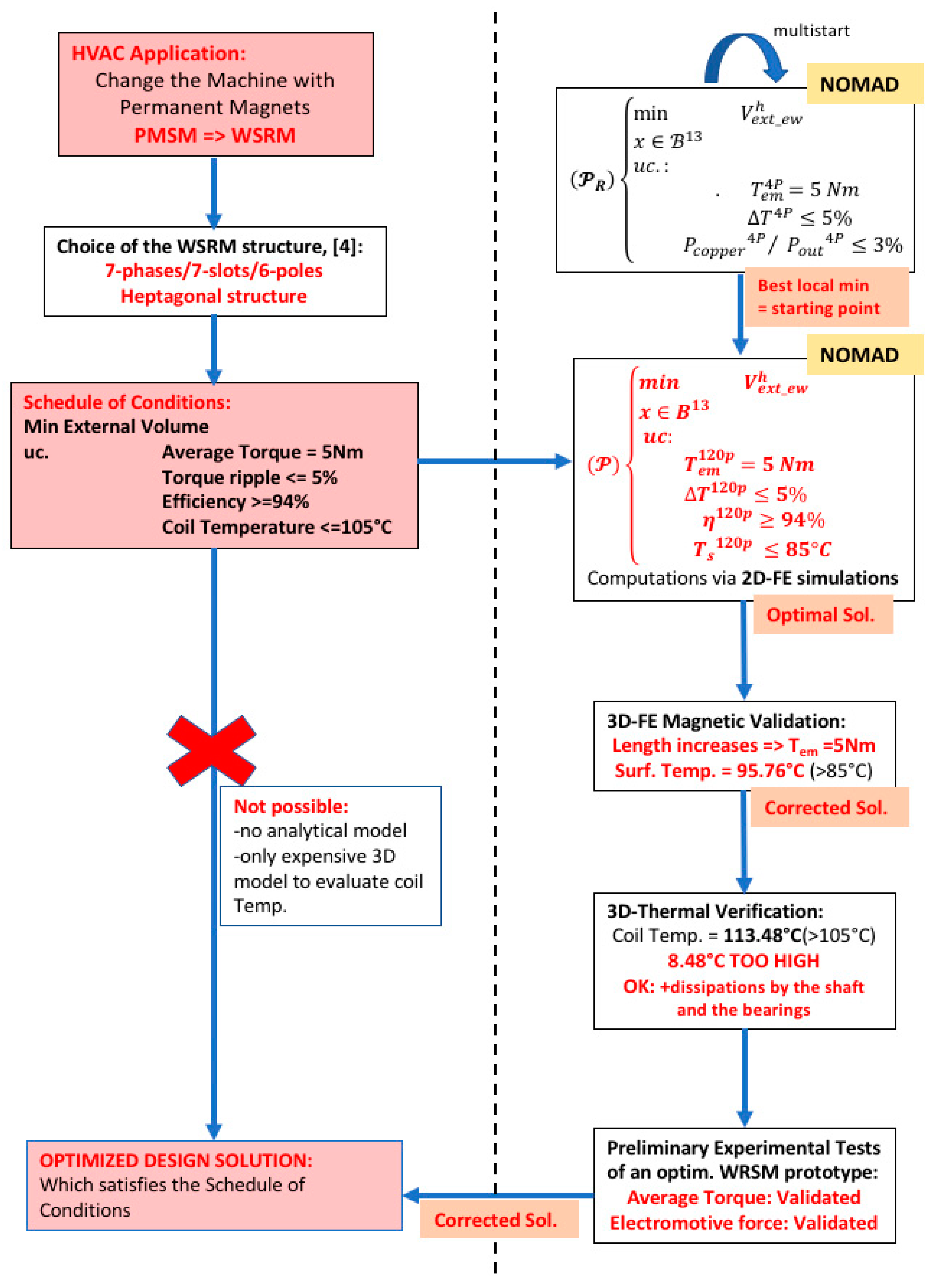
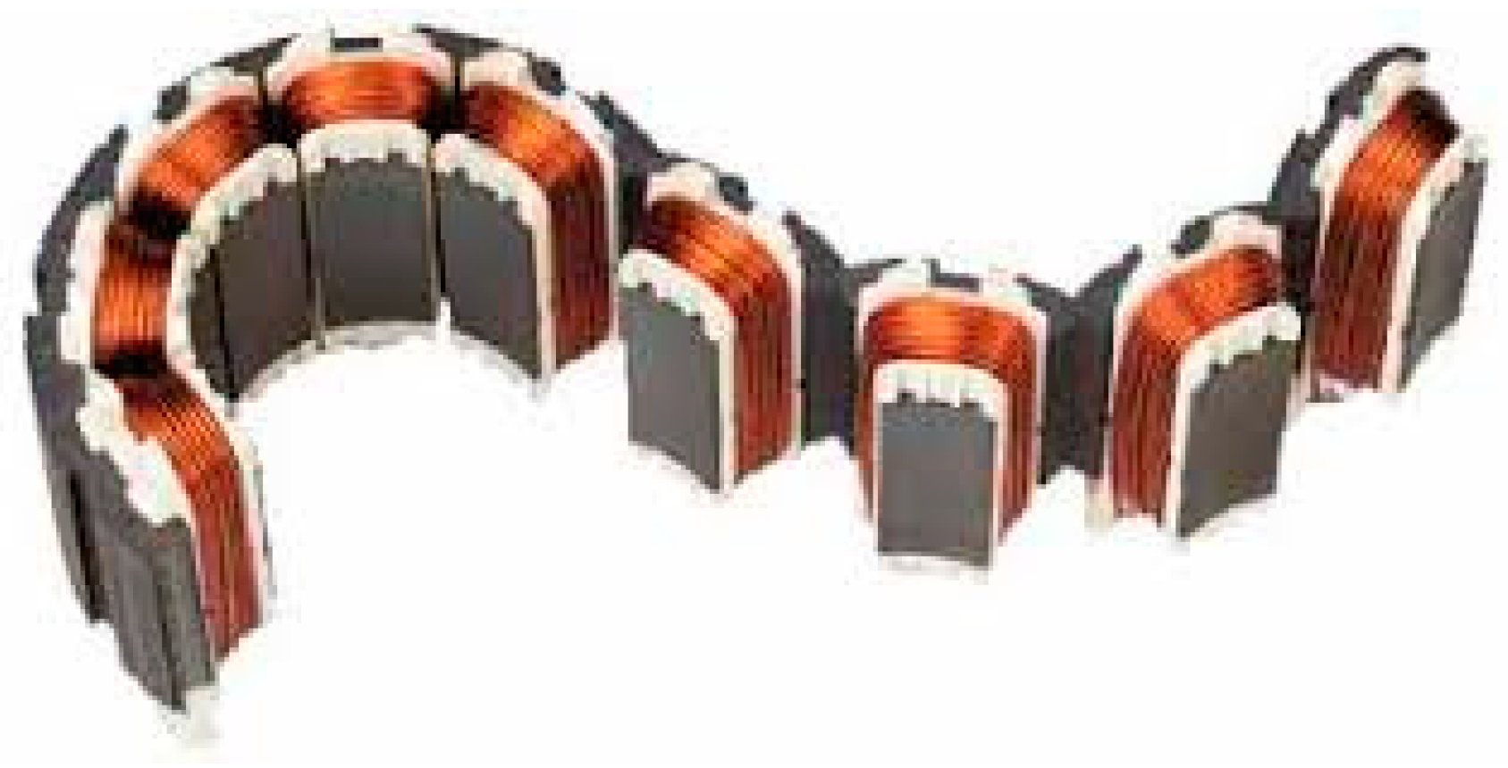
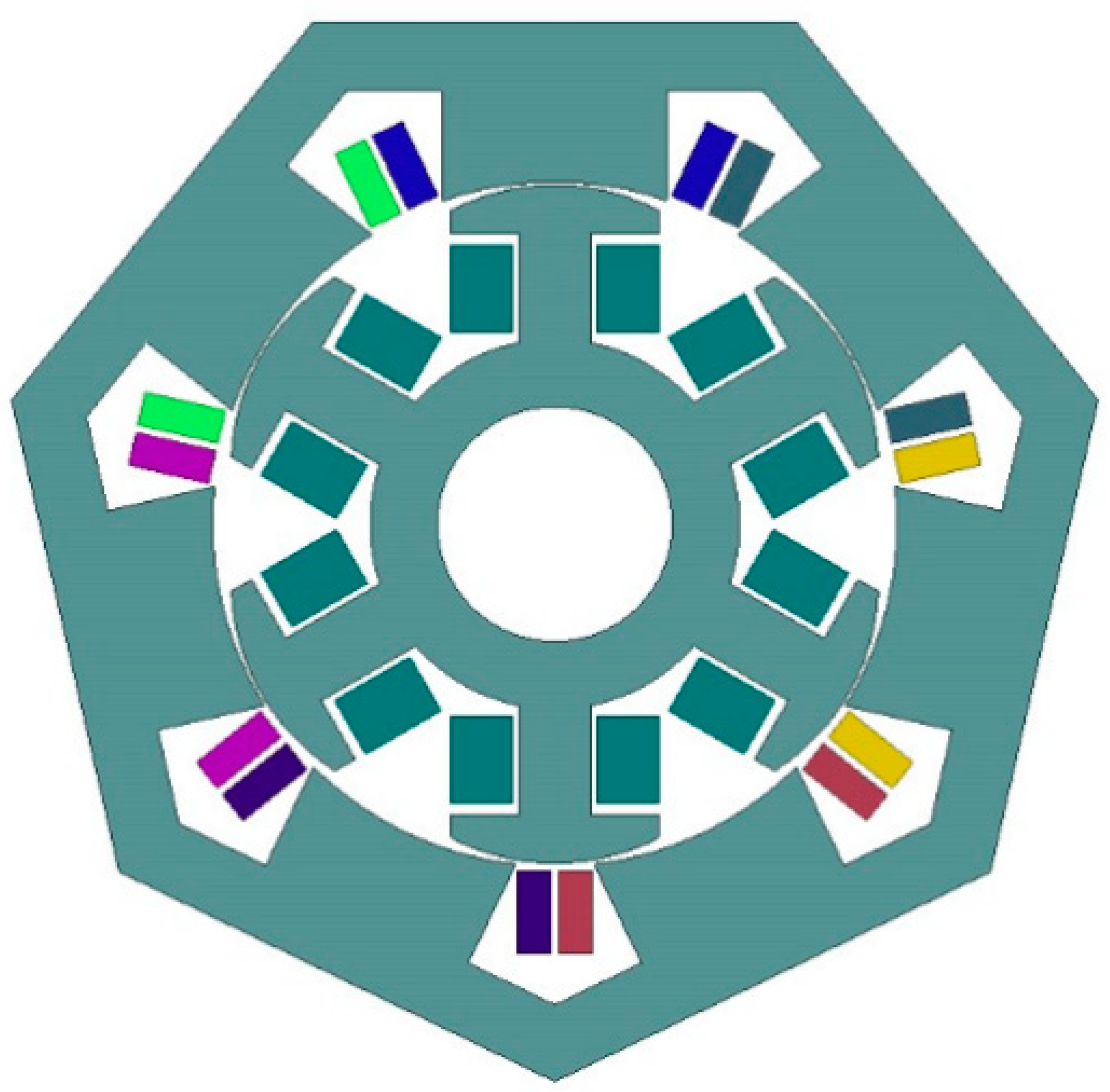
2. Optimization of a Heptagonal Based WRSM
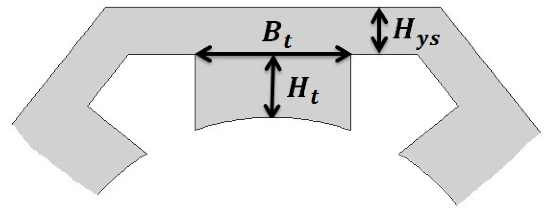
2.1. Variables
2.2. Objective Function
2.3. Inequality and Equality Constraints
- The torque ripple is defined by:
- The efficiency of the motor is determined by:
2.4. Optimization Problem
2.5. Optimization Algorithm: NOMAD
2.6. Starting Points
2.7. Optimization Results
2.8. Optimization Methodology
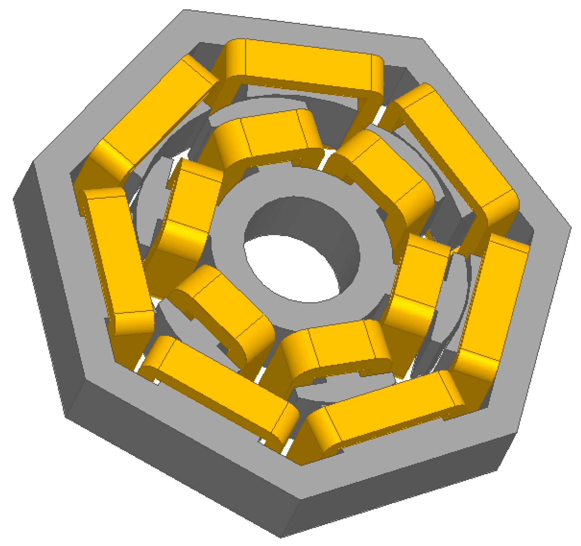
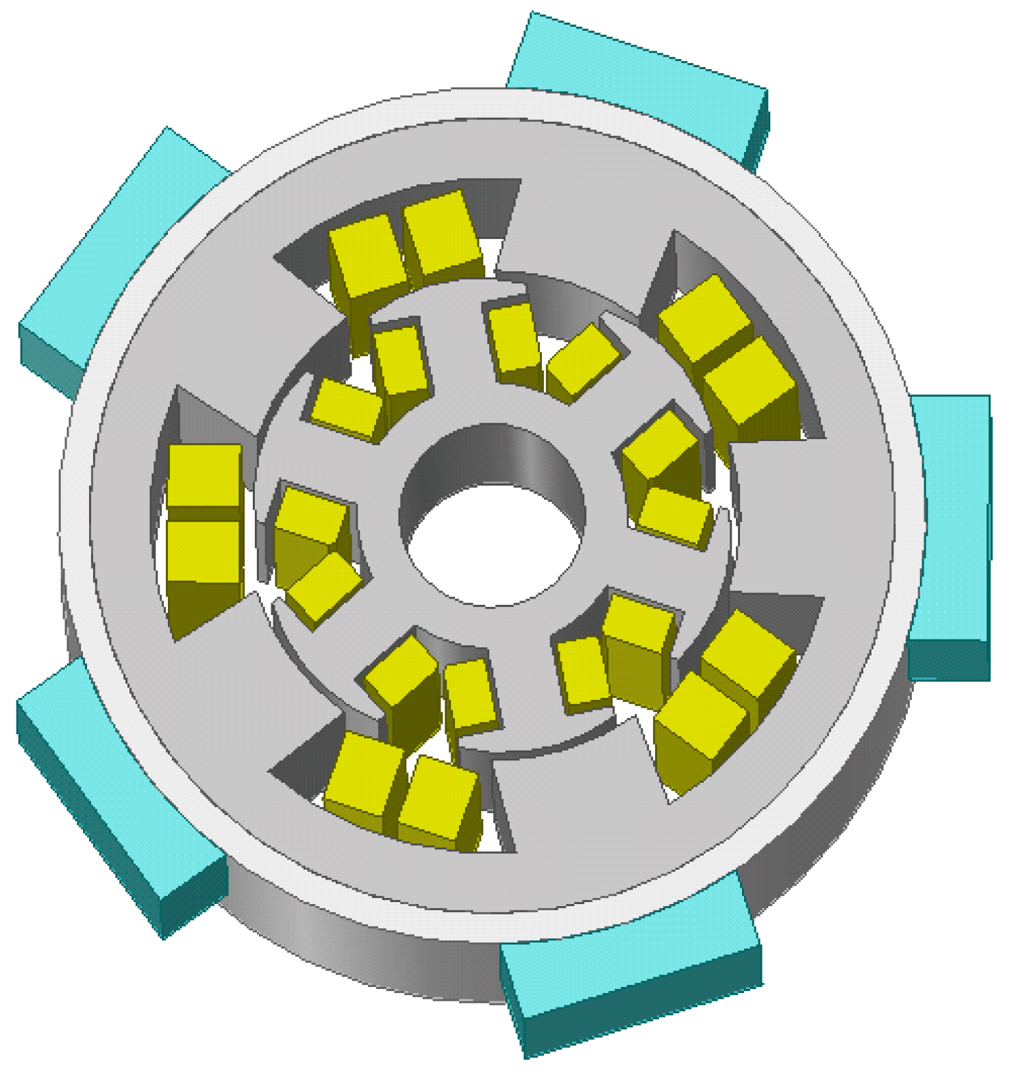
3. 3D Numerical Validations
3.1. Introduction
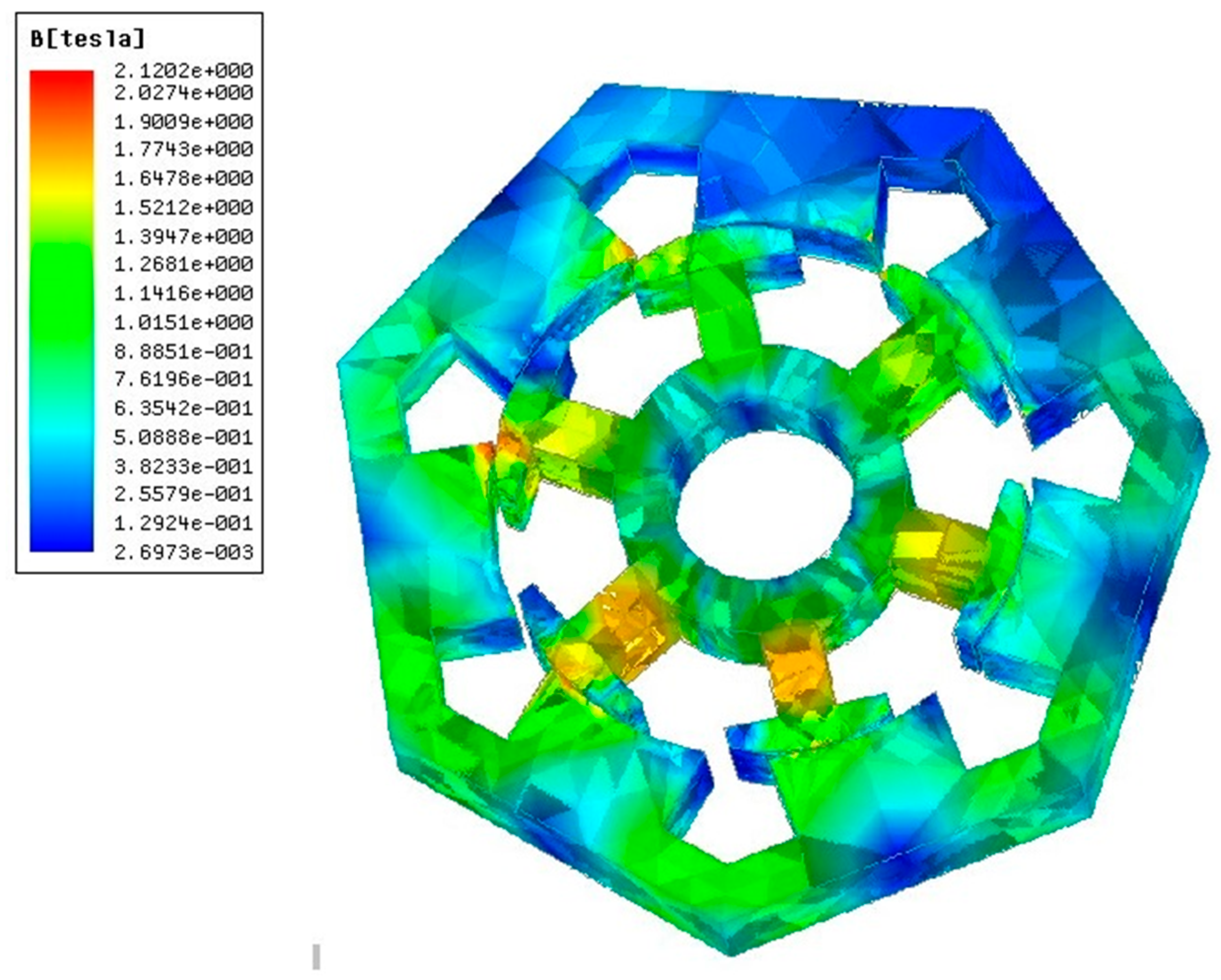
3.2. 3D Electromagnetic Verification
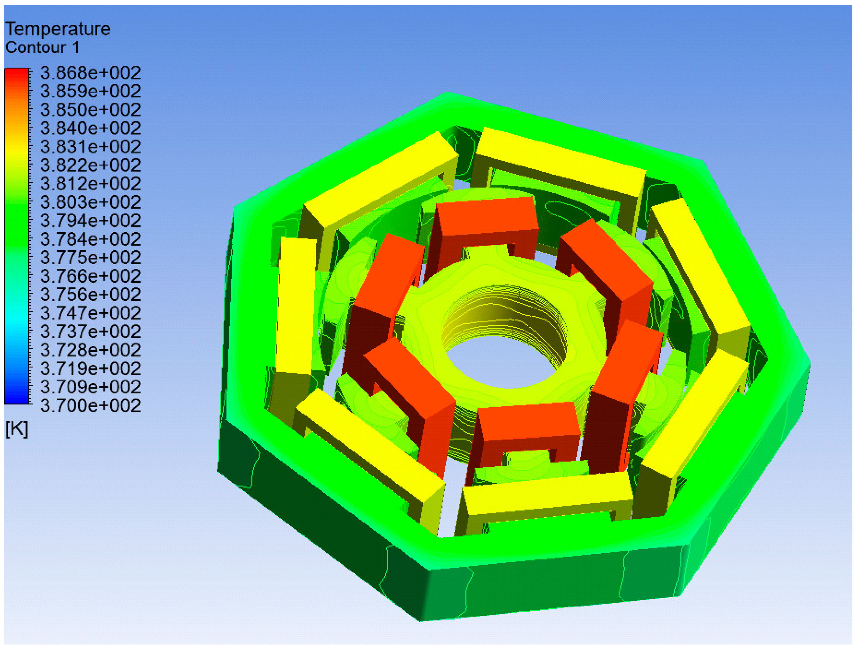
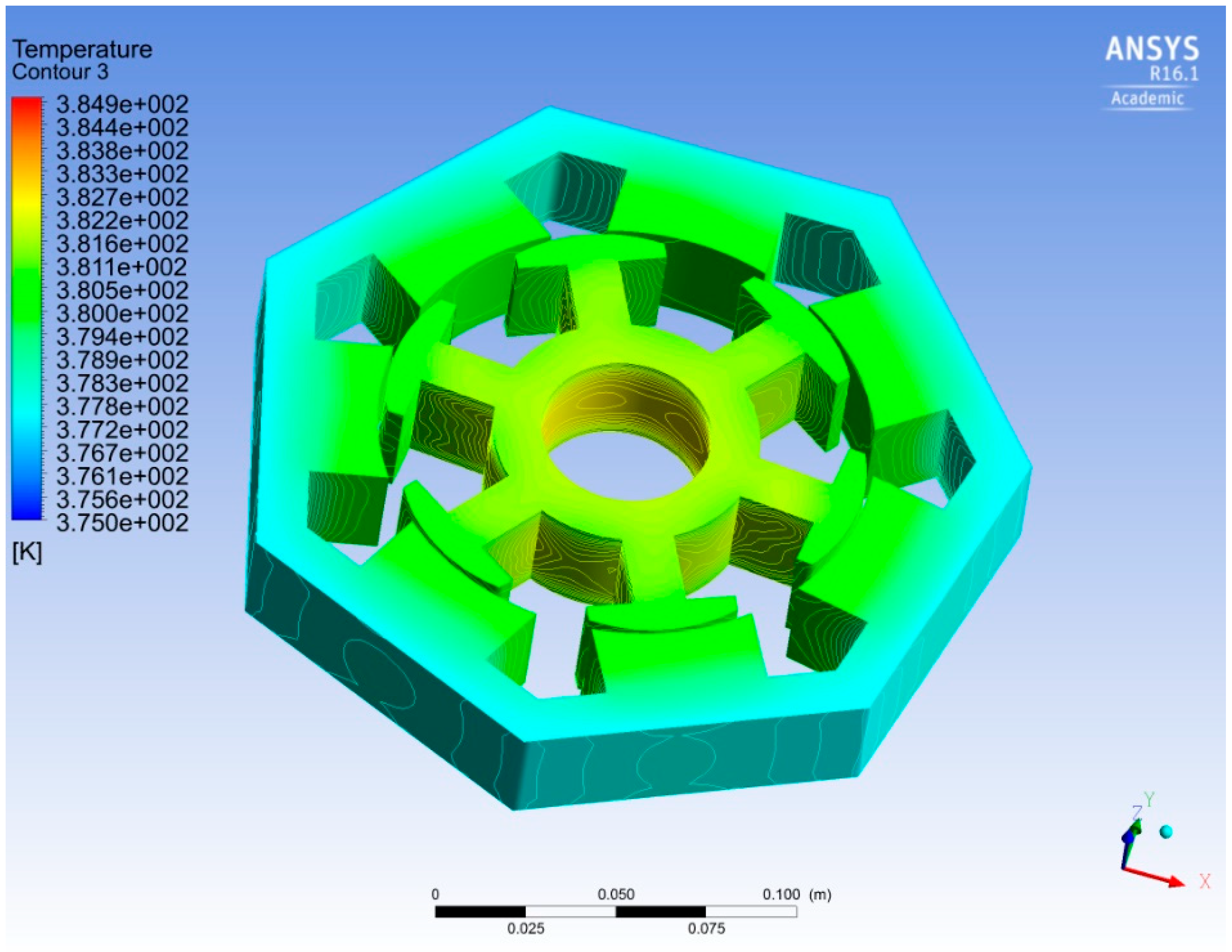
3.3. Thermal Analysis
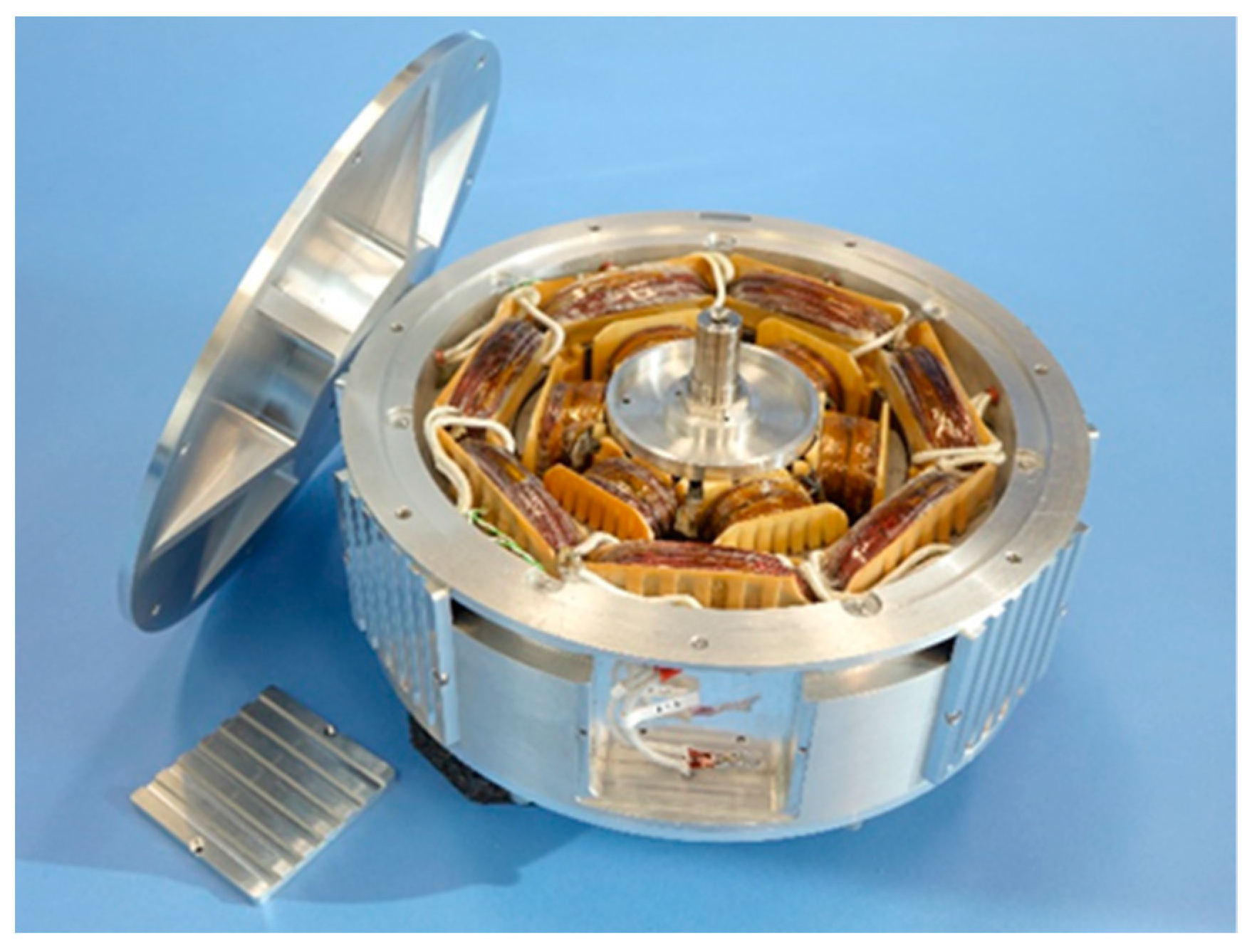
4. Preliminary Experimental Test
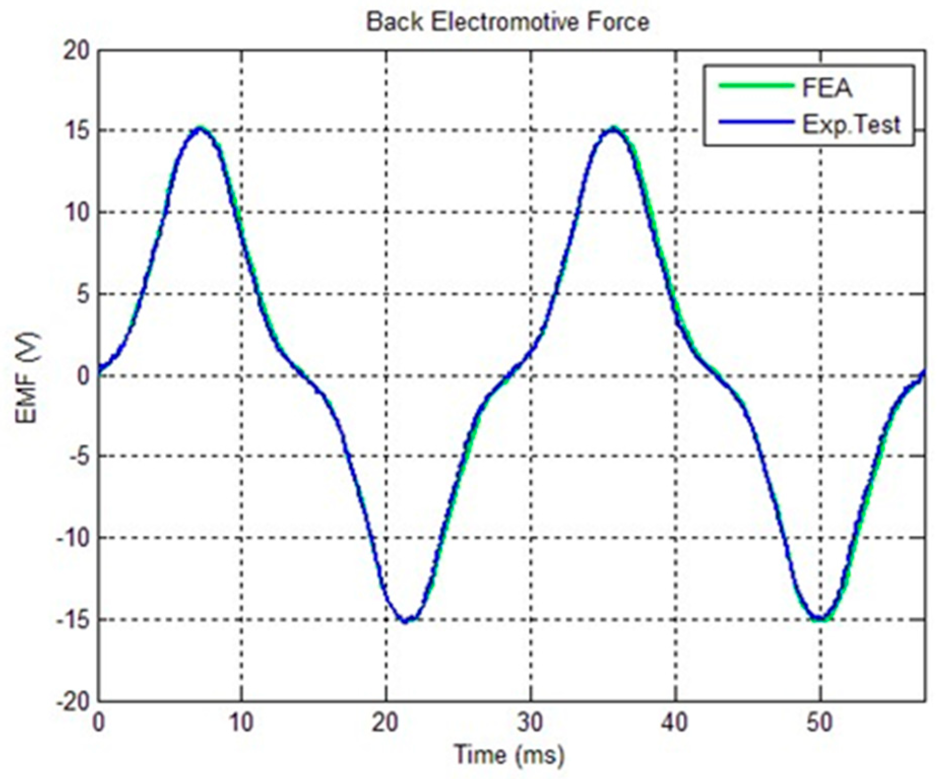
4.1. Electromotive Force at No Load
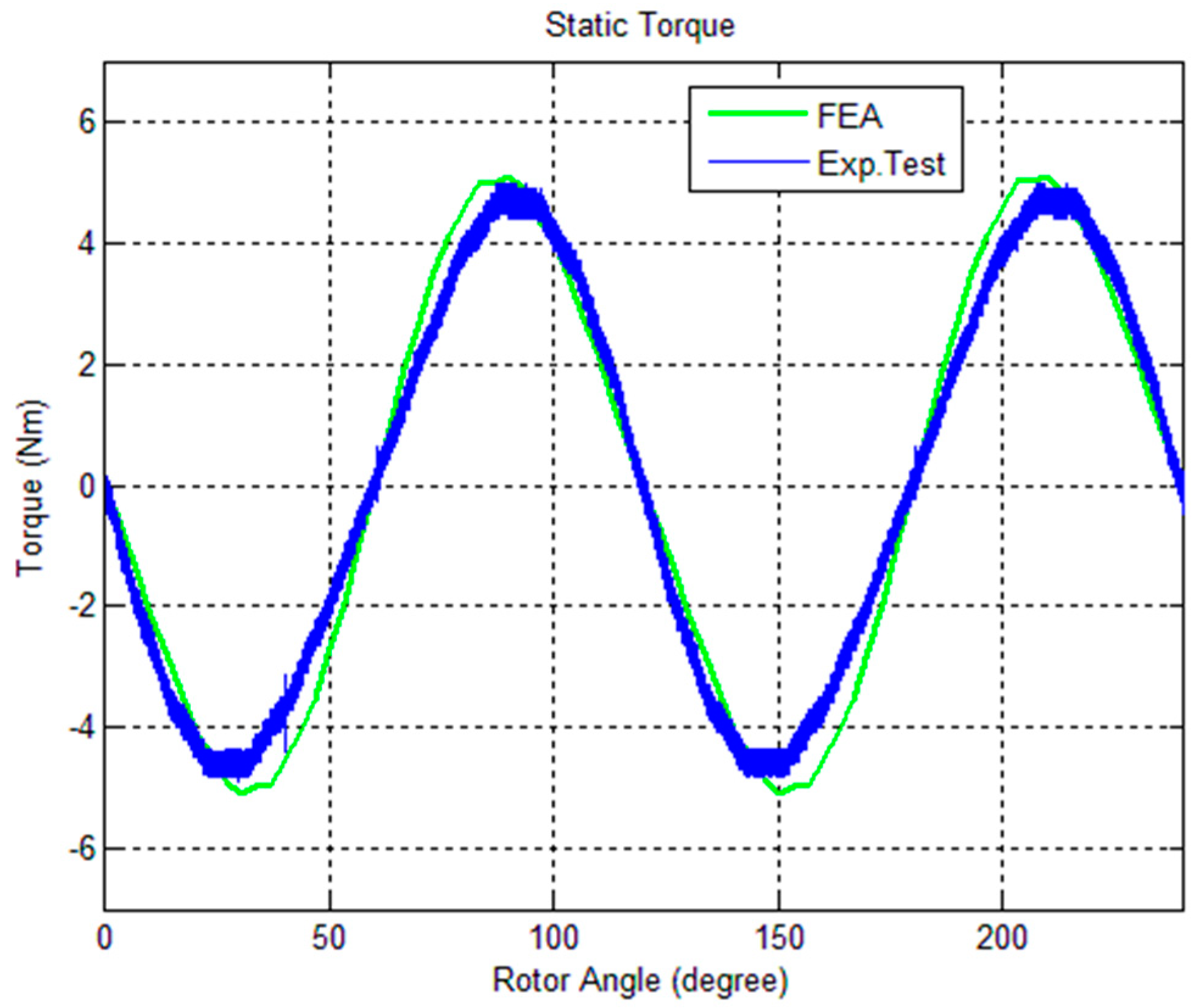
4.2. Static Torque vs. Rotor Angle
5. Conclusions
Supplementary Materials
Author Contributions
Funding
Institutional Review Board Statement
Informed Consent Statement
Conflicts of Interest
Appendix A
- Optimization,
- 3D Numerical Validations,
- Preliminary Experimental Tests on a Prototype.
References
- Rossi, C.; Casadei, D.; Pilati, A.; Marano, M. Wound Rotor Salient Pole Synchronous Machine Drive for Electric Traction. In Proceedings of the Industry Applications Conference, 41st IAS Annual Meeting, Tampa, FL, USA, 8–12 October 2006. Conference Record of the IEEE. [Google Scholar]
- Jürgens, J.; Brune, A.; Ponick, B. Electromagnetic Design and Analysis of a Salient Pole Synchronous Machine with Tooth-Coil Windings for Use as a Wheel Hub Motor in an Electric Vehicle. In Proceedings of the Electrical Machines (ICEM) Conference, Berlin, Germany, 2–5 September 2014. [Google Scholar]
- Liu, H.; Xu, L.; Shangguan, M. Finite element Method Simulation of a High Speed Wound Rotor Synchronous Machine. In Proceedings of the Electrical Machines and Systems (ICEMS) Conference, Beijing, China, 20–23 August 2011. [Google Scholar]
- Gündogdu, T.; Kömügöz, G. Implementation of Fractional Slot Concentrated Winding Technique in Large Salient-Pole Synchronous Generators. In Proceedings of the Power Electronics and Machines in Wind Applications (PEMWA), Denver, CO, USA, 16–18 July 2012. [Google Scholar]
- Topaloglu, I.; Ocak, C.; Tarimer, I. A case study of Getting Performance Characteristics of a Salient Pole Synchronous Hydro Generators. Elektron. Elektrotechnika 2010, 97, 57–61. [Google Scholar]
- Lin, D.; Zhou, P.; He, B.; Lambert, N. Steady state and transient parameter computation for wound field synchronous machines. In Proceedings of the Electrical Machines (ICEM) Conference, Marseille, France, 2–5 September 2012. [Google Scholar]
- Shipurkar, U.; Polinder, H.; Ferreira, J.A. Modularity in Wind Turbine Generator Systems—Opportunities and Challenges. In Proceedings of the 18 Europen Conference on Power Electronics and Application, Karlsruhe, Germany, 5–9 September 2016. [Google Scholar] [CrossRef]
- Li, G.; Zhu, Z.; Foster, P.; Stone, D.; Zhan, H. Modular Permanent-Magnet Machines with Alternate Teeth Having Tooth Tips. IEEE Trans. Ind. Electron. 2015, 62, 6120–6130. [Google Scholar] [CrossRef] [Green Version]
- Motor Technologies for Industry and Daily Life Edition; Mitsubishi Electric Advance, September 2003; Volume 103. Available online: https://www.advance.mitsubishielectric.com/advance/pdf/2003/vol103.pdf (accessed on 18 October 2021).
- The Current Status of and Future Trends in Heat Pump Technologies with Natural Refrigerants. Available online: http://www.mitsubishielectric.com/en/about/rd/advance/pdf/vol120/vol120.pdf (accessed on 18 October 2021).
- Le Luong, H.T.; Hénaux, C.; Messine, F.; Bueno-Mariani, G.; Voyer, N.; Mollov, S. Finite Element Analysis of a modular brushless wound rotor synchronous machine. In Proceedings of the 9th International Conference on Power Electronics, Machines and Drives, Liverpool, UK, 17–19 April 2018. [Google Scholar]
- Le Luong, H.T.; Messine, F.; Henaux, C.; Mariani, G.B.; Voyer, N.; Mollov, S. 3D Electromagnetic and Thermal Analysis for an Optimized Wound Rotor Synchronous Machine. In Proceedings of the 2018 XIII International Conference on Electrical Machines (ICEM), Alexandroupoli, Greece, 3–6 September 2018; pp. 455–460. [Google Scholar] [CrossRef]
- Liu, H.; Xu, L.; Shangguan, M.; Fu, W.N. Finite Element Analysis of 1 MW High Speed Wound-Rotor Synchronous Machine. IEEE Trans. Magn. 2012, 48, 4650–4653. [Google Scholar] [CrossRef]
- Le Digabel, S. Blackbox optimization with the NOMAD software, GERAD and Ecole Polytechnique de Montréal (MAGI), CanmetEnergie. ACM Trans. Math. Softw. 2015, 37, 1–15. [Google Scholar] [CrossRef]
- Audet, C.; Custodio, A.L.; Dennis, J.E., Jr. Erratum, Mesh adaptive direct search algorithms for constrained optimization. SIAM J. Optim. 2018, 18, 1501–1503. [Google Scholar] [CrossRef] [Green Version]
- Seo, M.; Lee, T.; Kim, J.; Kim, Y.; Jung, S. Principal Component Optimization with Mesh Adaptive Direct Search for Optimal Design of IPMSM. IEEE Trans. Magn. 2017, 53, 8105604. [Google Scholar] [CrossRef]
- Le Luong, H.T.; Messine, F.; Henaux, C.; Mariani, G.B.; Voyer, N.; Mollov, S. Comparison between fmincon and NOMAD Optimization Codes to Design Wound Rotor Synchronous Machines. Int. J. Appl. Electromagn. Mech. 2019, 60, S87–S100. [Google Scholar] [CrossRef]
- ANSYS Maxwell 2D/3D User’s Guide. Available online: http://ansoft-maxwell.narod.ru/english.html (accessed on 18 October 2021).
- Pyrhönen, J.; Jokinen, T.; Hrabovcova, V. Design of Rotating Electrical Machines; John Wiley & Sons, Ltd.: Hoboken, NJ, USA, 2008; ISBN 978-0-470-69516-6. [Google Scholar]
- Yeo, H.-K.; Park, H.-J.; Jung, S.-Y.; Ro, J.-S.; Jung, H.-K.; Seo, J.M. Electromagnetic and thermal analysis of a surface-mounted permanent-magnet motor with overhang structure. IEEE Trans. Magn. 2017, 53, 1–4. [Google Scholar] [CrossRef]
- Pechanek, R.; Kindl, V.; Skala, B. Transient thermal analysis of small squirrel cage motor through coupled FEA. Sci. J. 2015, 560–563. [Google Scholar] [CrossRef]
- Pechanek, R.; Bouzek, L. Analyzing of two types water cooling electric motors using computational fluid dynamics. In Proceedings of the 15th International Power Electronics and Motion Control Conference and Exposition, Novi Sad, Serbia, 4–6 September 2012. [Google Scholar]
- Fan, X.; Qu, R.; Li, J.; Li, D.; Zhang, B.; Wang, C. Ventilation and Thermal Improvement of Radial Forced Air-Cooled FSCW Permanent Magnet Synchronous Wind Generators. IEEE Trans. Ind. Appl. 2017, 53, 3447–3456. [Google Scholar] [CrossRef]
- Polikarpova, M. Liquid Cooling Solutions for Rotating Permanent Magnet Synchronous Machines. Ph.D. Thesis, Science at Lappeenranta University of Technology, Lappeenranta, Finland, 21 November 2014. [Google Scholar]
- Ding, S.; Li, H. Investigation of characteristics of fluid flow pattern for air-cooled motor. In Proceedings of the 2016 IEEE 11th Conference on Industrial Electronics and Applications (ICIEA), Hefei, China, 5–7 June 2016; pp. 2044–2048. [Google Scholar] [CrossRef]
- Connor, P.H.; Pickering, S.J.; Gerada, C.; Eastwick, C.N.; Micallef, C.; Tighe, C. Computational fluid dynamics modelling of an entire synchronous generator for improved thermal management. IET Electr. Power Appl. 2013, 7, 231–236. [Google Scholar] [CrossRef]
- Connor, P.; Pickering, S.; Gerada, C.; Eastwick, C.; Micallef, C. CFD modelling of an entire synchronous generator for improved thermal management. In Proceedings of the 6th IET International Conference on Power Electronics, Machines and Drives (PEMD 2012), Bristol, UK, 27–29 March 2012. [Google Scholar] [CrossRef] [Green Version]
- SanAndres, U.; Almandoz, G.; Poza, J.; Ugalde, G. Design of Cooling Systems Using Computational Fluid Dynamics and Analytical Thermal Models. IEEE Trans. Ind. Electron. 2013, 61, 4383–4391. [Google Scholar] [CrossRef]


| Name | Symbol | Unit | Bounds on B |
|---|---|---|---|
| Machine length | mm | B1 = [20; 60] | |
| Stator yoke height | mm | B2 = [05; 20] | |
| Tooth height | mm | B3 = [08; 30] | |
| Tooth width | mm | B4 = [20; 50] | |
| Rotor yoke height | mm | B5 = [05; 20] | |
| Pole shoe height | mm | B6 = [03; 20] | |
| Pole shoe width | mm | B7 = [20; 60] | |
| Pole body height | mm | B8 = [10; 35] | |
| Pole body width | mm | B9 = [10; 30] | |
| Pole arc offset | mm | B10 = [20; 90] | |
| Shaft diameter | mm | B11 = [0; 30] | |
| Armature current density | B12 = [0; 6] | ||
| Field current density | B13 = [0; 4] |
| Symbol | Name | Relation |
|---|---|---|
| Average torque | ||
| Torque ripple | ||
| Efficiency | ||
| Surface temperature |
| Variable | Starting Point for | Optimal Design | Unit |
|---|---|---|---|
| Machine length | 39.92 | 31.62 | mm |
| Stator yoke height | 9.33 | 13.95 | mm |
| Tooth height | 13.21 | 18.38 | mm |
| Tooth width | 30.82 | 45.46 | mm |
| Rotor yoke height | 8.75 | 12.88 | mm |
| Pole shoe height | 5.30 | 9.80 | mm |
| Pole shoe width | 39.39 | 41.90 | mm |
| Pole body height | 16.35 | 22.14 | mm |
| Pole body width | 23.81 | 14.50 | mm |
| Shaft diameter | 43.18 | 47.53 | mm |
| Pole arc offset | 7.12 | 23.18 | mm |
| Armature current density | 4.36 | 2.69 | |
| Field current density | 6.27 | 3.87 |
| Performance | Unit | ||
|---|---|---|---|
| Average torque | 4.99 | 4.9977 | Nm |
| Torque ripple | 3.35% | 3.51% | |
| Total losses | 223 | 162.46 | W |
| Efficiency | 94.16% | 95.56% | |
| Temperature | 151.11 | 85 | °C |
| Performance | Value | Unit |
|---|---|---|
| Average torque | 4.84 | Nm |
| Torque ripple | 4.28% | |
| Phase Voltage (rms) | 91.74 | V |
| Total losses | 192.28 | W |
| Efficiency | 94.79% | |
| Temperature | 95.75 | °C |
| Performance | Value | Unit |
|---|---|---|
| Average torque | 5 | Nm |
| Torque ripple | 4.05% | |
| Phase Voltage (rms) | 94.27 | V |
| Stator copper losses | 35.80 | W |
| Rotor copper losses | 51.51 | W |
| Iron losses | 105.94 | W |
| Efficiency | 94.89% | |
| Temperature | 96.07 | °C |
| Material | Conductivity | Capacity | Density |
|---|---|---|---|
| Lamination | Radial (28) | 420 | 7650 |
| Axial (2) | |||
| Copper | 387 | 380 | 8960 |
| Polyimide | 0.26 | 1000 | 1449 |
| Steel | 16.27 | 502.48 | 8030 |
| Aluminium | 202.4 | 871 | 2719 |
| Air | 0.026 | 1000 | 1.22 |
| Phase Current | Theoretical Value (A) t = 0 | Measured Value (A) |
|---|---|---|
| 8.87 | 8.79 | |
| 5.53 | 5.53 | |
| −1.97 | −1.97 | |
| −7.99 | −7.99 | |
| −7.99 | −7.99 | |
| −1.97 | −1.97 | |
| 5.53 | 5.53 |
| Steps | Experimental Test | 2D FE Analysis |
|---|---|---|
| 0(IAmax) | 4.97 | 5.07 |
| π/35 | 5.13 | 5.06 |
| 2π/35 | 5.04 | 5.08 |
| 3π/35 | 5.16 | 5.08 |
| 4π/35 | 4.95 | 5.03 |
| 5π/35 | 5.06 | 5.03 |
| 6π/35 | 5.20 | 5.06 |
| 7π/35 | 5.11 | 5.08 |
| 8π/35 | 5.06 | 5.08 |
| 9π/35 | 5.10 | 5.03 |
| 10π/35 (IBmax) | 5.13 | 5.02 |
Publisher’s Note: MDPI stays neutral with regard to jurisdictional claims in published maps and institutional affiliations. |
© 2021 by the authors. Licensee MDPI, Basel, Switzerland. This article is an open access article distributed under the terms and conditions of the Creative Commons Attribution (CC BY) license (https://creativecommons.org/licenses/by/4.0/).
Share and Cite
Le Luong, H.T.; Messine, F.; Hénaux, C.; Mariani, G.B.; Voyer, N.; Mollov, S.; Harribey, D. Optimization, 3D-Numerical Validations and Preliminary Experimental Tests of a Wound Rotor Synchronous Machine. Energies 2021, 14, 8118. https://doi.org/10.3390/en14238118
Le Luong HT, Messine F, Hénaux C, Mariani GB, Voyer N, Mollov S, Harribey D. Optimization, 3D-Numerical Validations and Preliminary Experimental Tests of a Wound Rotor Synchronous Machine. Energies. 2021; 14(23):8118. https://doi.org/10.3390/en14238118
Chicago/Turabian StyleLe Luong, Huong Thao, Frédéric Messine, Carole Hénaux, Guilherme Bueno Mariani, Nicolas Voyer, Stefan Mollov, and Dominique Harribey. 2021. "Optimization, 3D-Numerical Validations and Preliminary Experimental Tests of a Wound Rotor Synchronous Machine" Energies 14, no. 23: 8118. https://doi.org/10.3390/en14238118
APA StyleLe Luong, H. T., Messine, F., Hénaux, C., Mariani, G. B., Voyer, N., Mollov, S., & Harribey, D. (2021). Optimization, 3D-Numerical Validations and Preliminary Experimental Tests of a Wound Rotor Synchronous Machine. Energies, 14(23), 8118. https://doi.org/10.3390/en14238118