Thermal Fluxes and Solar Energy Storage in a Massive Brick Wall in Natural Conditions

Abstract

The thermal state of building elements is a combination of steady and transient states. Changes in temperature and energy streams in the wall of the building in the transient state are particularly intense in its outer layer. The factors causing them are solar radiation, ambient temperature and long-wave radiation. Due to the greater variability of these factors during the summer, the importance of the transient state increases at this time. The study analysed heat transfer in three aspects, temperatures in the outer, middle and inner parts of the wall, heat fluxes between these layers and absorption of solar energy, heat transfer coefficient on the wall exterior was also calculated. The analysis is based on temperature measurements at several depths in the wall and measurements of solar radiation. The subject of research is a solid brick wall. The results show that the characteristics of heat flow in winter and summer for the local climate show distinct differences. In the winter, the maximum temperature difference between the external and internal surface of the wall was 10 °C and in summer, 20 °C. In the winter, the negative flux on the internal surface reached 10 W/m² and on the external 40 W/m² and was constant throughout the day. The mean heat transfer coefficient on the exterior surface for winter week was 8 W/(mK). A Nusselt and Biot number for dimensionless convection analysis was calculated. The research contributes to the calculation of the variability of heat or cold demand in a daily period and to learn about the processes of energy storage in the wall using sensible heat.

1. Introduction

Transient changes in temperature and heat fluxes in the building partition affect the energy demand for heating and cooling as well as the mechanical durability of the element. Modelling of these changes has been the subject of many theoretical and numerical works, a review of which can be found in [1]. Generally, steady-state heat transfer models are used to calculate heating energy demand in buildings. For large temperature changes in the summer period, the dynamics of temperature variation in the wall should be taken into account. These algorithms are used to optimise HVAC systems.

The current procedures of heat balance calculations in Poland and Europe include solar gains through opaque walls, and therefore partially take into account the dynamics of heat flow [2]. Completely dynamic calculations are included in [3], the admittance method is usually used to describe temperature variations. In this method, harmonic changes in temperature are assumed. In fact, the temperature course depends on the azimuth of the wall, its coverage by surrounding objects, and the weather conditions on a given day. In order to obtain the temperature data to be used in the simulations, the obtained measurement results can be transformed by a Fourier transform into the frequency domain.

A comparison of the static and dynamic approach is presented in [4]. The aim of this article is to describe heat fluxes and temperatures in a brick wall in natural conditions, based on measurements. The experiment was carried out in a moderate climate in summer and winter conditions. The heat fluxes are important for the heating and cooling appliances design. Wall surface temperature changes influence the durability of the outer layers of the facade. The high heat capacity of the wall causes a reduction in temperature amplitude and a phase shift. Solar energy is stored in the wall and returned to the room after a few hours.

Observations of the temperature variability and heat fluxes in the wall during summer and winter time were examined. A period of two example weeks, taken from January–August 2021 was analysed. Heat is exchanged between the wall and the external environment through convection as well as thermal and solar radiation [5]. Convection also occurs on the inside. Inner convection is mainly due to buoyancy forces and is less intense than outer convection forced by the wind and greater temperature differences between the wall and air.

Inside the wall, heat flows mainly through conduction. The problem of the temperature course and heat fluxes in a multi-layer wall was dealt with in [6], where the Authors developed a method for calculating the wall surface temperature using measurements and validating a numerical model with them. The research on the influence of the solar radiation absorption coefficient on the temperature in the wall was carried out in [7]. It was shown that increasing the absorbency of the surface from zero to one causes an increase in its temperature by about 8 °C at the intensity of solar radiation of 400 W/m² at peak. The conclusions from [6,7,8] indicate that solar radiation has a significant influence on the temperature of the outer wall surface. The ability to absorb this radiation is determined by the absorption coefficient. The list of coefficients depending on the type of surface is presented in [9]. Wall measured in this article is covered with plaster in the upper part and darker ceramic tiles in the lower part. Solar absorbance of those tiles is expected to be higher than plaster raising temperature on the bottom of the wall. The high absorbency of the wall is beneficial in winter as it increases solar gains. In summer, however, it increases the demand for cooling the building, or the temperature in rooms increases beyond the comfort zone. The solution to this problem may be to make an external covering with low absorbency or to plant cover plants that give shadow in summer. This reduces the energy for air conditioning and at the same time does not cut off the solar gain in winter.

The effect of shading with vegetation was described in [10]. It was shown that in this way it is possible to reduce the maximum temperature of the wall surface by about 5 degrees. The wall examined in this article was also partially covered by a tree and the shadow effects were clearly visible. Cyclical cooling and heating of the wall affect its durability, especially in historic buildings [11]. The wall can act as a solar energy store, in order to increase its storage capacity, PCM materials [12,13] or liquids with high heat capacity [14] can be used. Additionally, the materials can be optimised at the molecular level to achieve the desired properties [15,16,17,18]. With a thick wall made of high-density material, the sensible heat storage in the structure itself may be sufficient.

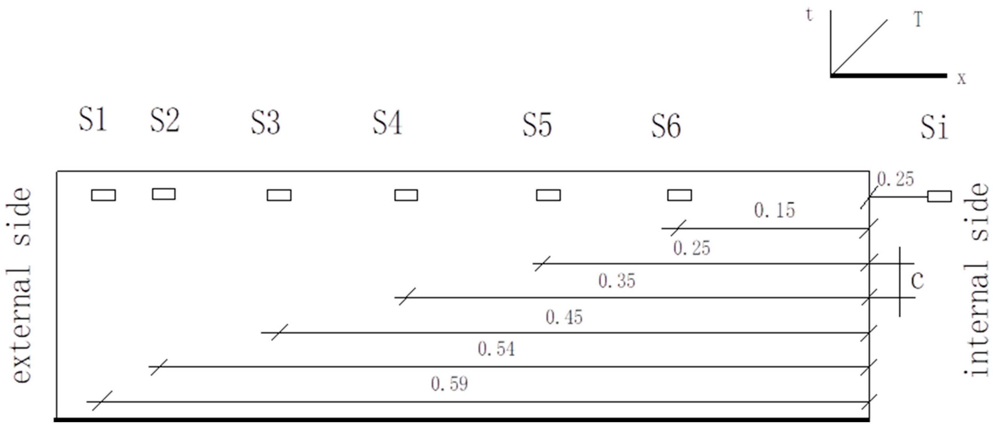
2. Materials and Methods

The assessed wall belongs to the facade of one of the University buildings, built in the 1930s. It is a massive, 60 cm thick partition made of solid brick, its normal facing almost directly SE, azimuth 129°. It does not have thermal insulation and was treated in the research as single layer. It was covered with a light cream-coloured plaster, at the bottom lined with brown ceramic facade tiles. It has semiconductor temperature sensors Pt1000 at several depths as shown in Figure 1. Measurements were performed using the setup described in detail in [19,20,21]. The sensors are positioned with spacing c = 10 cm apart parallel to the wall. It was assumed that the temperature distribution across the wall is unchanged and the sensors are treated as placed along one axis.

The coordinate system can be described in terms of wall coordinate x, time t and temperature T (x,t).

This arrangement of sensors was installed from 1 January to 26 April 2021. Later, the S1 temperature sensor was removed due to the commencement of renovation of the facade. During the renovation, measurements with the other sensors were continued, the layer of façade tiles with a thickness of about 2 cm was removed, but the analyses omitted to change the thickness and, at the same time, the thermal capacity of the wall as small. On the inside, there is a didactic and research laboratory where construction materials, mainly concrete mixtures, are tested. The room was heated in the winter, the time of switching on and switching off the heating was not measured. Through the acquisition of measurements, we create a recorded temperature field.

Measurements of the thermal properties of bricks removed from the wall during the renovation were carried out with the use of the ISOMET 2114 device. The dimensions of the brick were 0.27 × 0.13 × 0.06 m, which is typical for bricks produced before the Second World War. Density was obtained by direct method by measuring the mass and volume of the sample. The results are summarised in

Table 1. Thermal properties of bricks from the described wall.

Measurement No.	1	2	3	Mean
Thermal conductivity [W/(mK)]	0.9948	1.0146	1.0166	1.01
Volumetric specific heat [J/(m3K)]	1.6703 × 106	1.6743 × 106	1.6754 × 106	1.6733 × 106
Thermal diffusivity [m2/s]	0.5956 × 10−6	0.6060 × 10−6	0.6068 × 10−6	0.6028 × 10−6
Density [kg/m3]	1412	1412	1412	1412
Specific heat [J/(kgK)]	1183	1186	1187	1185

.

The obtained parameter values correspond to medium weight clay brick [22], however, a significantly higher thermal conductivity coefficient was recorded. A similar value of the coefficient was recorded in [23] by making measurements for the entire wall, both bricks and binder (mortar). Dry and saturated state brick parameters were measured in [24], the average value of these results corresponds to the value obtained in this study.

The microscopic photos of the brick sample are shown in Figure 2.

The brick structure is fine-grained with numerous inclusions, they are probably of clay origin. The pores visible in the figure on the right are approximately 0.3 mm in size and one pores approximately 1.5 mm in diameter. The pore area covers 11% of the field of view. The analysis of the structure of bricks before and after firing can be found in [25]. The observed structure of bricks corresponds to the description contained in the paper, no chemical analysis was performed.

In addition, in the period of 18 January–26 April, the intensity of solar radiation was measured using a meter cooperating with the same LB-480 logger by LAB-EL used for temperature recording. The sensor had to be removed because of the facade renovation. Due to the orientation of the wall, the maximum radiation occurs in the morning hours. The wall is partially sheltered by bushes and trees, limiting the incoming radiation, even on a clear day. The view of the wall with the solar radiation sensor and the sensor’s field of view are shown in Figure 3. The photo was taken on 26 April 2021 at 10:05 a.m. The results are therefore representative for any surface of wall covered with vegetation [26,27].

The obtained temperature values from the recorded field were approximated by a third-degree polynomial and then the regular field of temperature was calculated. The coordinate system corresponds to that adopted in [28]. Each of the calculated temperatures represents the average temperature of an element with a width of Δx equal to one centimeter. The elements are numbered from 1 to 60 as shown in Figure 4. The approximated temperature distribution contains values in regular spacing in contrast to measures values, so it was named “regular temperature grid”. Temperature T_i, n denotes the temperature approximated at point i (i = 1… 60) at time n.

The coefficient of determination was calculated for each profile to check the quality of the fit. This parameter can be used to check goodness of fit not only in linear regressions [29]. The total sum of squares is calculated from Equation (1)

$$S{S}_{tot,t}={\displaystyle \sum }_i{\left(y_{i,t}-\overline{y_t}\right)}^2.$$

(1)

where y_i,t—values measured for individual points at time t,—mean for all points at time t. Residual sum of squares

$$S{S}_{res,t}={\displaystyle \sum }_i{\left(y_{i,t}-f_{i,t}\right)}^2.$$

(2)

where y_{i, t}—values measured for individual points in time t, f_i,t—value of the fitting for these points. Coefficient of determination (COD) is calculated by Equation (3)

$$R_t^2=1-\frac{S{S}_{res,t}}{S{S}_{tot,t}}$$

(3)

The minimum and maximum values of the coefficient of determination for the measured data series were calculated. The Coefficient of Determination value close to one means a better fit of the approximation function to the measurements. Its value can be interpreted as a percentage of the variability of the measured value that can be predicted using the obtained approximating function.

Since the wall was assumed to be one layer, the properties of all cells are identical. The wall was divided into three zones. The outer zone consists of elements from 60 to 41 inclusive, the middle one consists of cells 40 to 21 and the inner one is from 20 to 1. These zones are denoted ext, mid, int.

3. Results

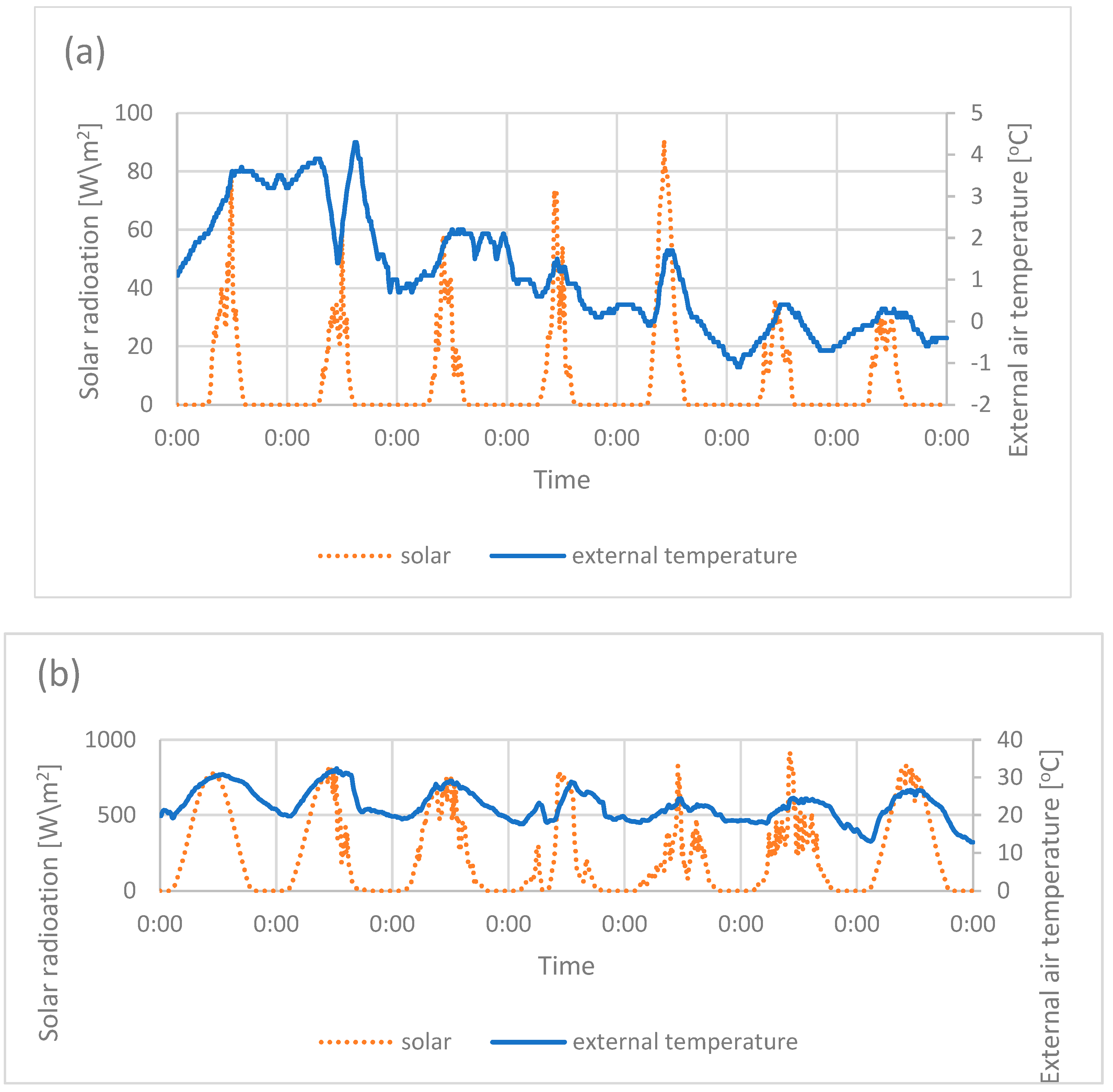
3.1. External Conditions

Two measurement periods were developed, each one week long. Winter conditions are represented by the week of 4–10 January 2021 and summer conditions by 21–27 June 2021. Temperatures were recorded in 10 min spacing. The charts of the outside air temperature and solar radiation for the horizontal surface for the winter week are shown in Figure 5a and for the summer week in Figure 5b.

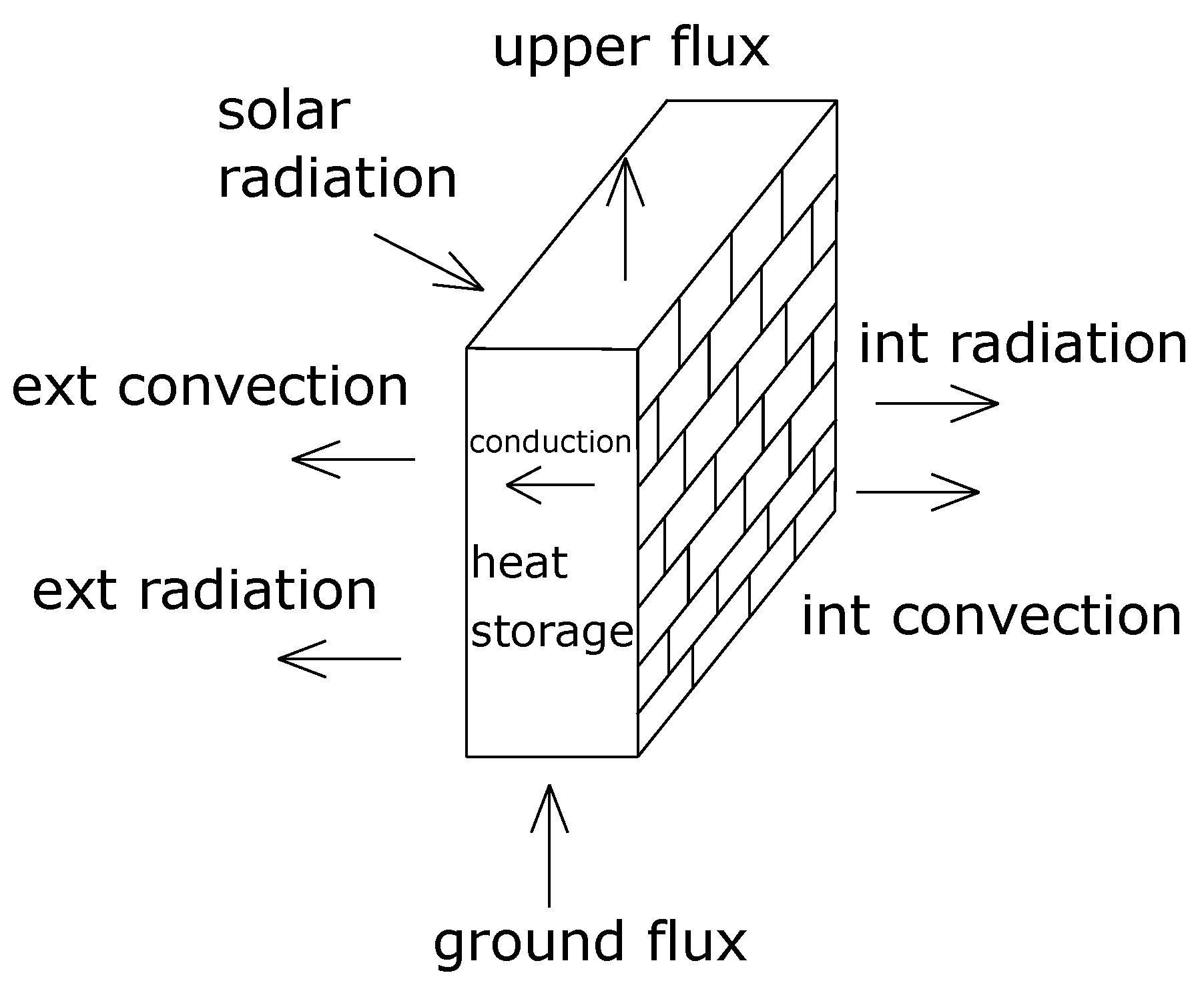
3.2. Energy Balance of the Wall

There are nine main heat fluxes in the wall, outside and inside exchange by convection and radiation, inside flow by conduction, heat storage in the wall, solar radiation and the fluxes from the lower level (ground) and to the upper storey. These heat fluxes are shown in Figure 6.

To verify the influence of ground flux and upper flux, measurements of the temperature above and below the plane in which the sensors are placed. There are no such sensors in the current measurement campaign, but they were installed in the previous measurements. They were mounted 10 cm above and below the sensor S4. The sensors were labeled S4U (above) and S4D (below). Since the wall is treated as a single material, the temperature difference enables a qualitative assessment of the heat flux. Figure 7 shows the temperature differences S4D-S4 and S4U-S4 in 23–30 January 2020 and Figure 8 in the period of 21–27 June 2020. In both figures, a negative sign means that the heat flux flows from node S4 and a positive sign that it flows towards it.

In the winter heat flows from the S4 sensor both up and down, flow to the ground is more intensive because the ground temperature is lower than upper parts of the buildings. In the summer the fluxes are more complicated. The flow tends to be unidirectional from bottom to top. It is probably not influenced by the temperature of the ground, but by the dark colour of the tiles at the bottom of the wall, which causes it to heat up more from the bottom. This phenomenon was expected as stated in the introduction.

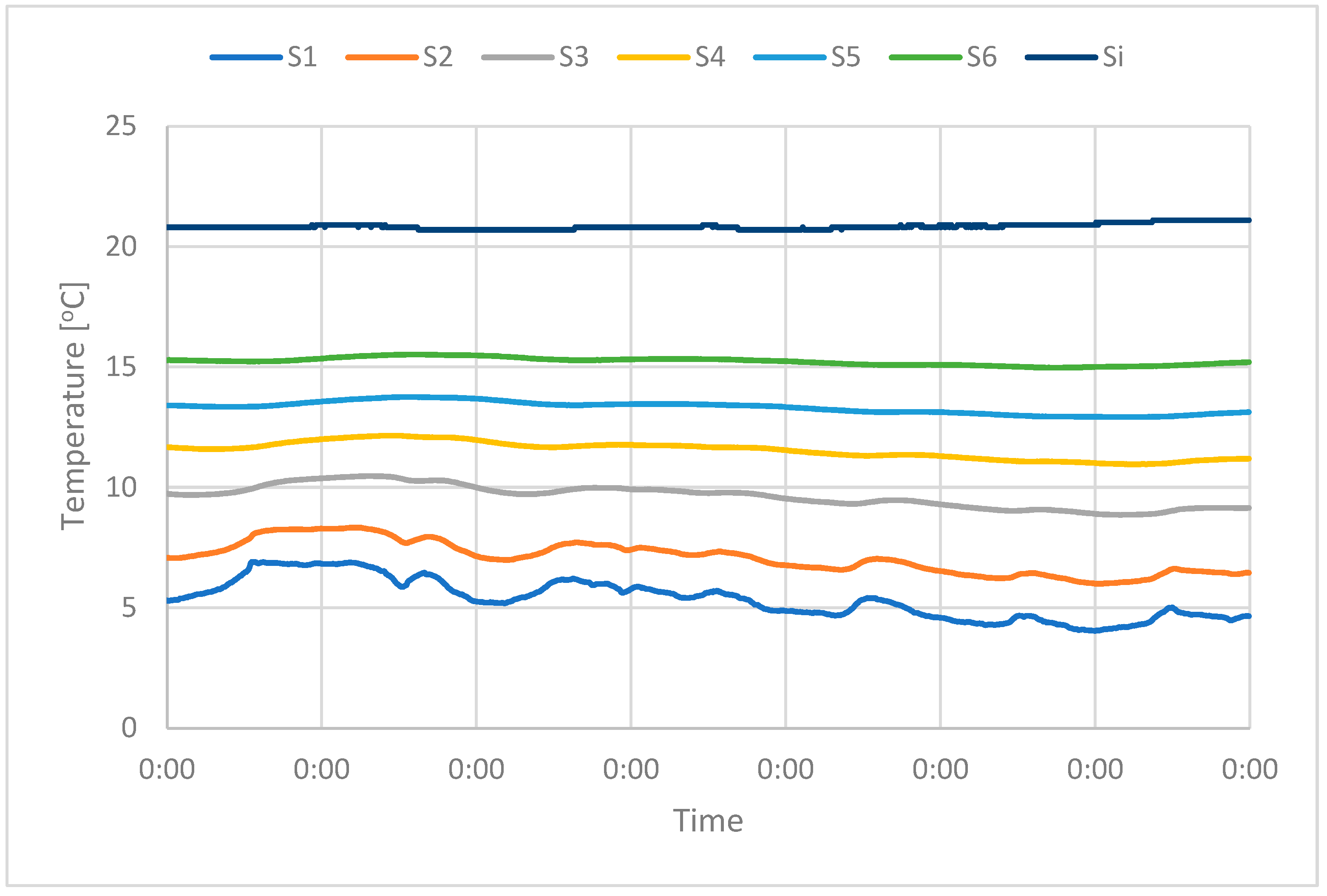
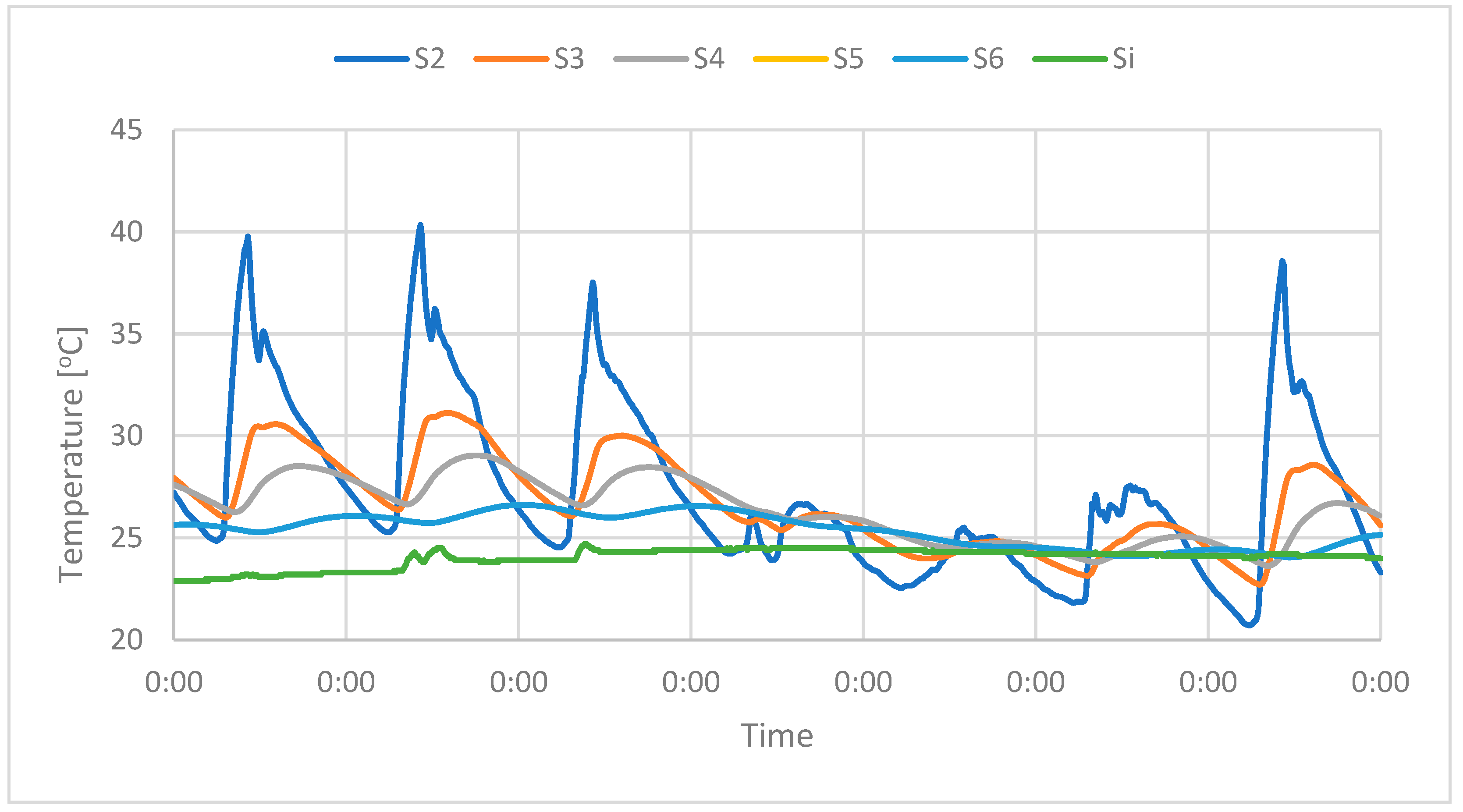
3.3. Recorded Temperatures

Recorded sensor temperatures for 4–10 January 2021 are shown in Figure 9.

Sensor temperatures for 21–27 June 2021 are shown in Figure 10. Sensor S1 was removed from its position and its temperature is no longer considered.

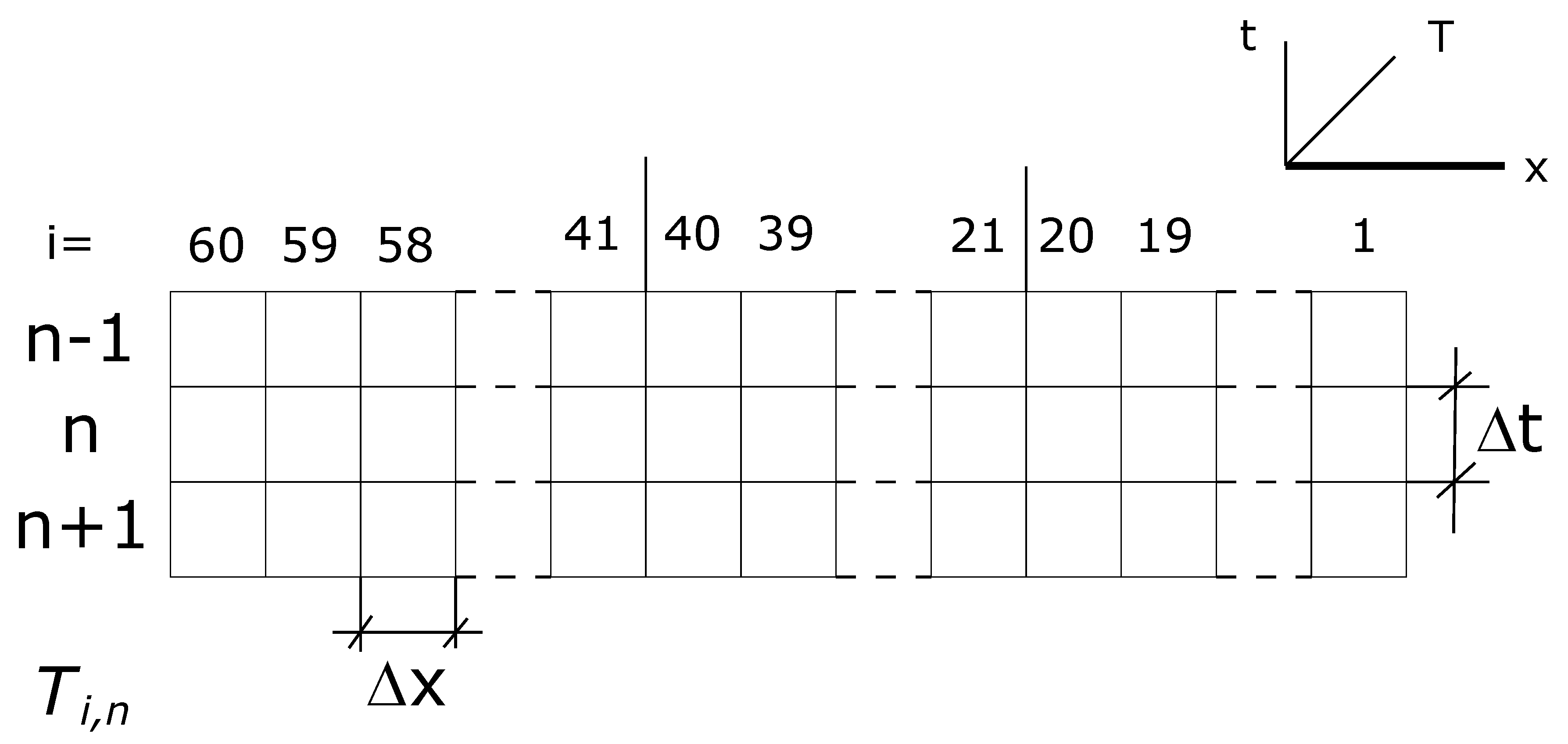
3.4. Data Fitting by Nonlinear Regression

Temperature approximations were made in Excel using the mean square method. In order to reduce the amount of data in a single sheet, it was performed independently for each month. The functions were obtained for each stored temperature profile in the wall. The average fit parameters for each week are presented in

Table 2. Goodness of fit parameters of wall temperature for individual weeks.

COD	4–10 January	21–27 June
R2 min	0.9987	0.5627
R2 max	0.9997	0.9999
R2 avg	0.9992	0.9817

.

The obtained regression approximates the measurements well. In winter, when the temperature profile is more stable, the fit is particularly good. As summer approaches, the temperature changes faster in the wall, mainly due to solar heating. This is the reason that for some moments the fit is weaker but the mean value still does not fall below 98% percent.

The greatest temperature variation occurs in the outer layer. The middle and inner layers are characterised by the smallest temperature fluctuations during the hour and day, especially in the summer. The course of temperature on a sunny summer day using the example of 22 June is explained in Figure 11.

The temperature of the outer layer rises during the hours of solar operation on the wall and as the temperature of the outside air increases. Due to the solar gains through the windows, the room temperature also rises, which in turn heats the inner layer of the wall. The increase in temperature of the inner layer is overestimated due to an approximation error during rapid heating of the outer layer. Then the heat is transferred to the middle layer. The temperature increase in this layer is, however, is staggered over time because it is stabilised by the heat capacity of the inner and outer layers.

In winter, the average temperature in individual layers is subject to much smaller changes. In the run for 5 January presented in Figure 12, it can be considered constant.

Figure 7 shows that the outdoor temperature variation was not greater than 3 °C during the whole week.

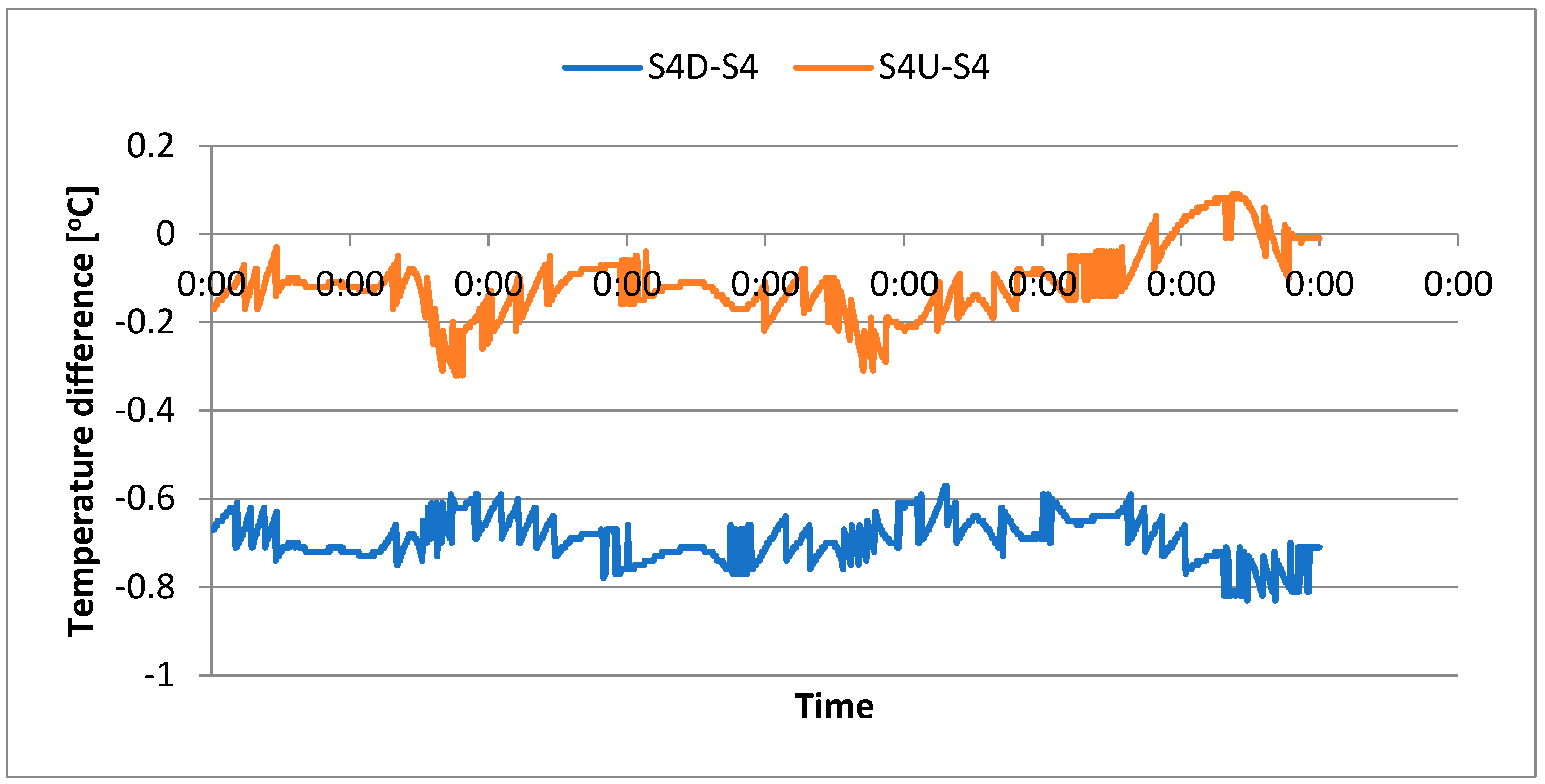
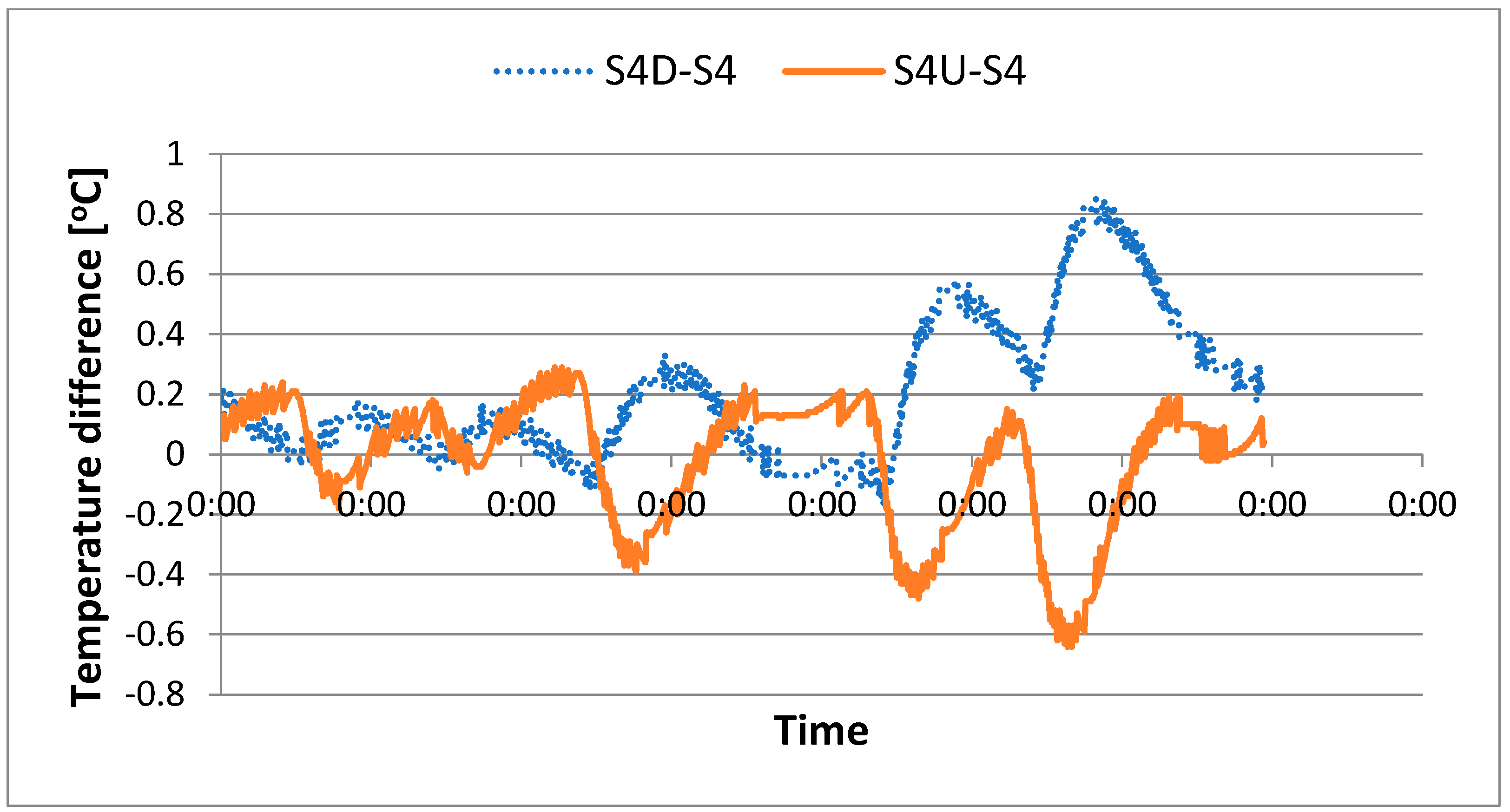
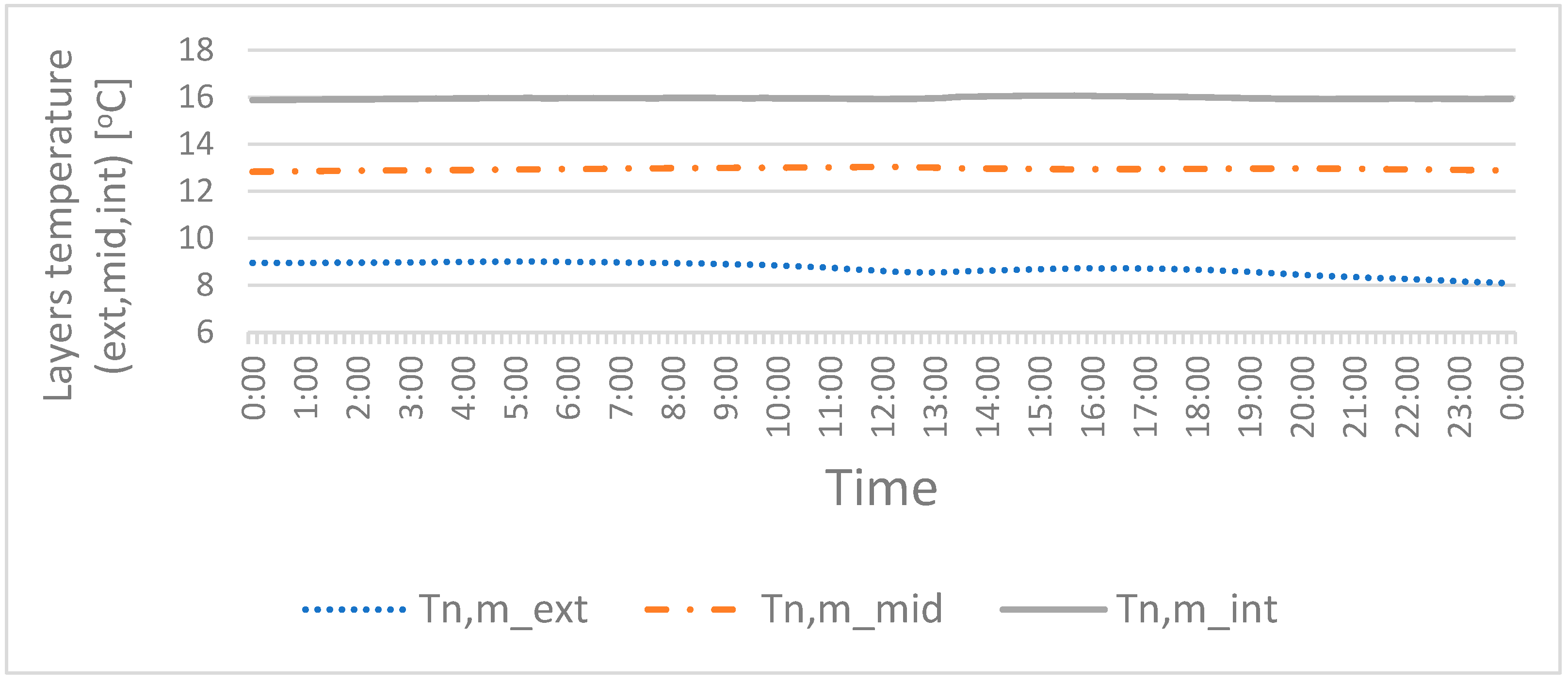
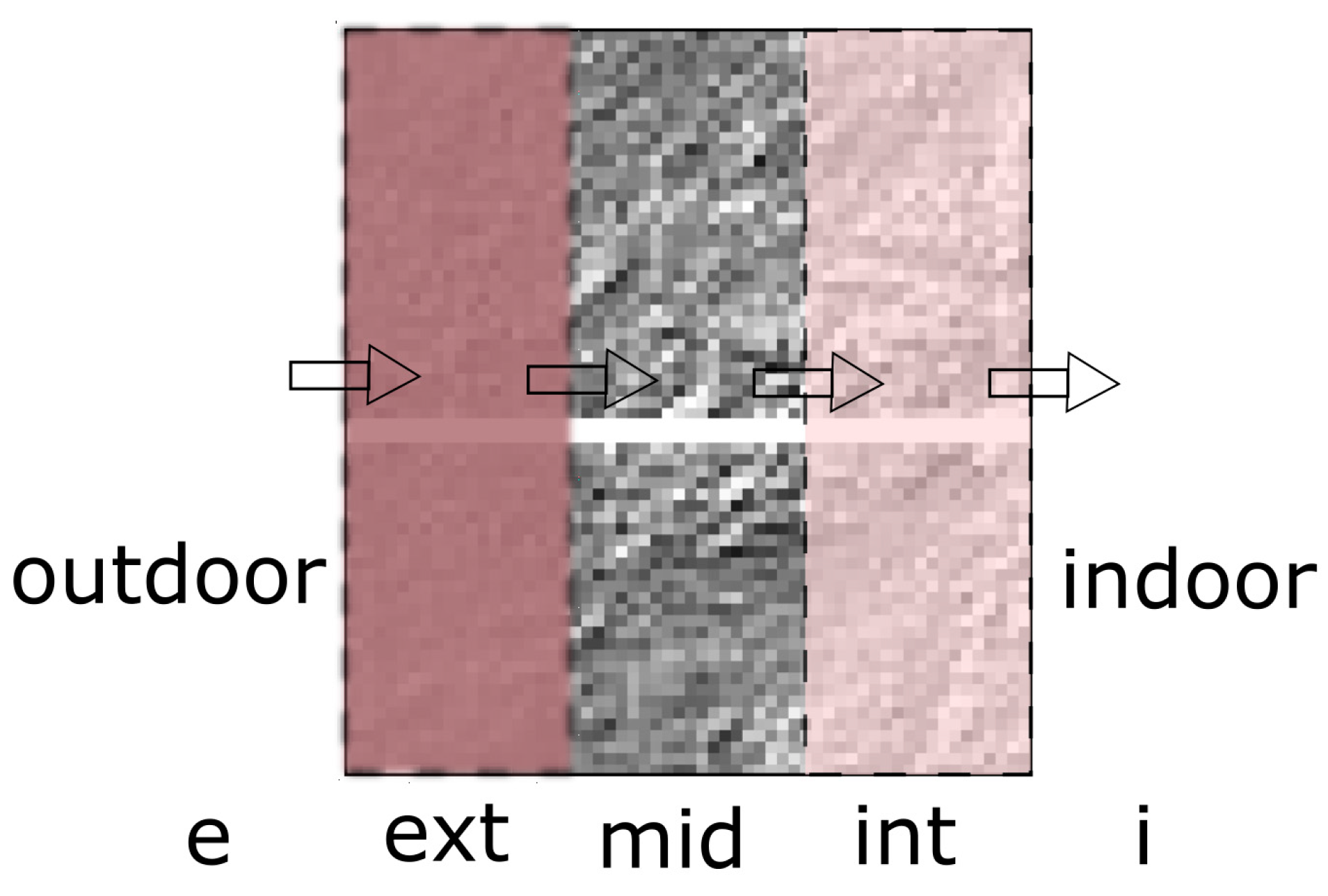
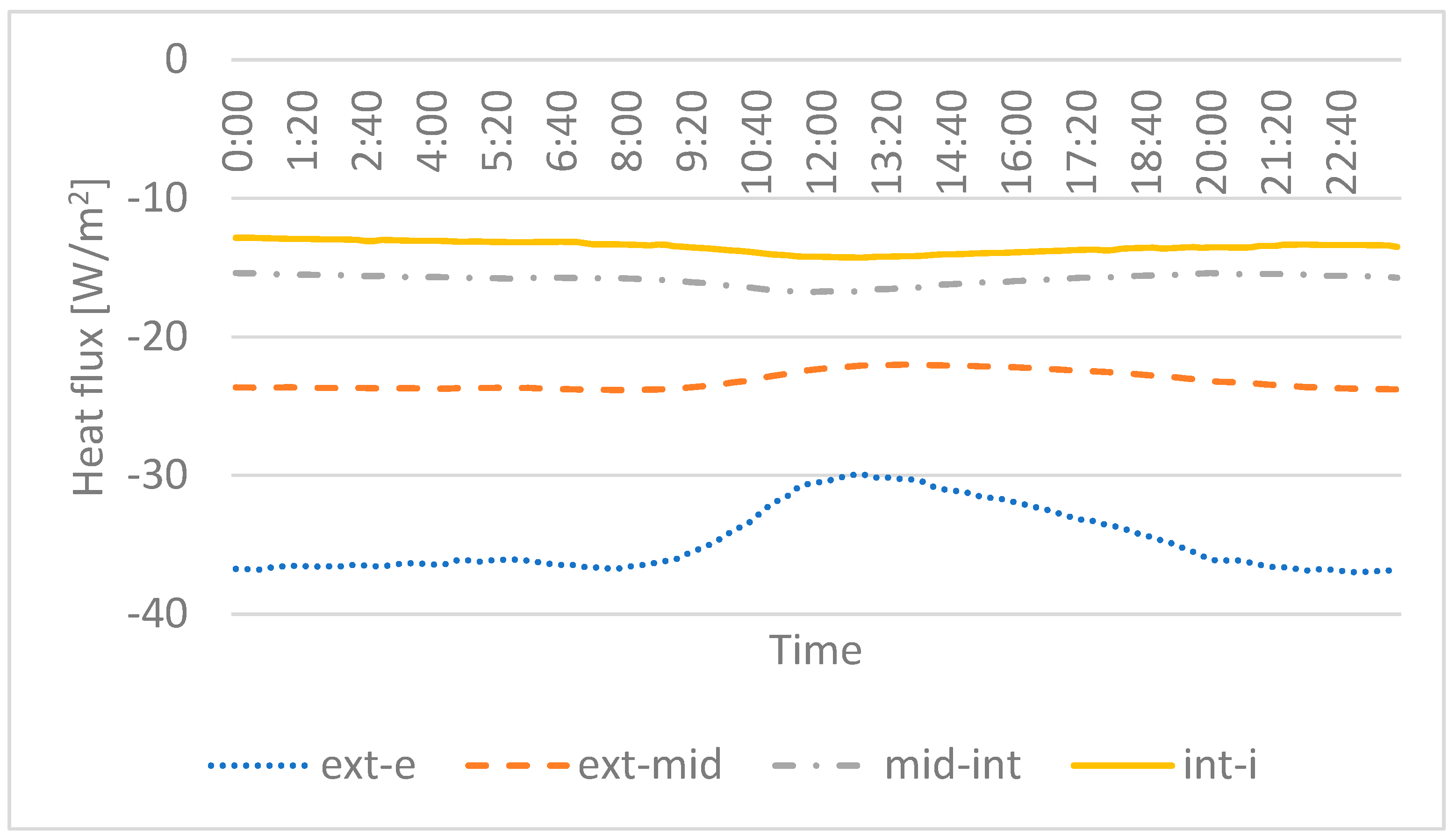
3.5. Heat Fluxes between Layers

Four control surfaces were distinguished on the edges of the wall and between the layers. The heat flux through these surfaces can be calculated

$$q=\frac{\lambda }{\mathsf{\Delta }x}\left(T_{n,i}-T_{n,j}\right).$$

(4)

where λ is the thermal conductivity coefficient a T_n,i and T_n,j of the temperature of the elements at the layer boundary. The boundary element numbers for individual control surfaces are summarised in

Table 3. Numbers of boundary elements in individual wall layers.

Control Surface	i	j
ext-e	60	59
ext-mid	41	40
mid-int	21	20
int-i	2	1

.

The directions of heat fluxes assumed as positive according to the numbering in Table 3 are shown in Figure 13.

The value of the thermal conductivity coefficient of the wall was adopted for the measurements of a single brick. Heat fluxes were analysed for 27 June 2021 and for an exemplary summer day and 8 January 2021 for a winter day. The chart for 27 June is shown in Figure 14.

According to the drawing, the positive heat flux on the ext-e surface means the heat flows into the wall, and on the int-i surface inversely. The heat flux flows into the wall from both sides due to solar radiation and internal temperature. This stream then flows across the boundary between the outer and middle layers. A stream of heat enters the wall also from the inside. In the evening hours, the heat drains off, especially outside the wall. Approximately 5 h after the maximum flux flowing to the wall through the ext-e surfaces, the direction of heat flow through the int-i surfaces changes and the room is heated [31].

The chart for 8 January is shown in Figure 15.

The flux exchanged by the outer wall surface is negative for 24 h a day, therefore it has the direction of heat escape from the wall. The incident solar radiation reduces the net loss but does not change the flow direction. The stream from inside the room is also negative, which means, however, that the wall is heated from the inside. The power of this heating is about three times less than the power of external losses. Comparing the results with [32], it can be seen that in this study greater differences between summer and winter were obtained. It is caused by more different values of solar radiation and outside temperature. The heat flux flowing between the middle and inner layers is greater than between the inner environment and the wall surface. This is probably the influence of the boundary conditions in the previous days.

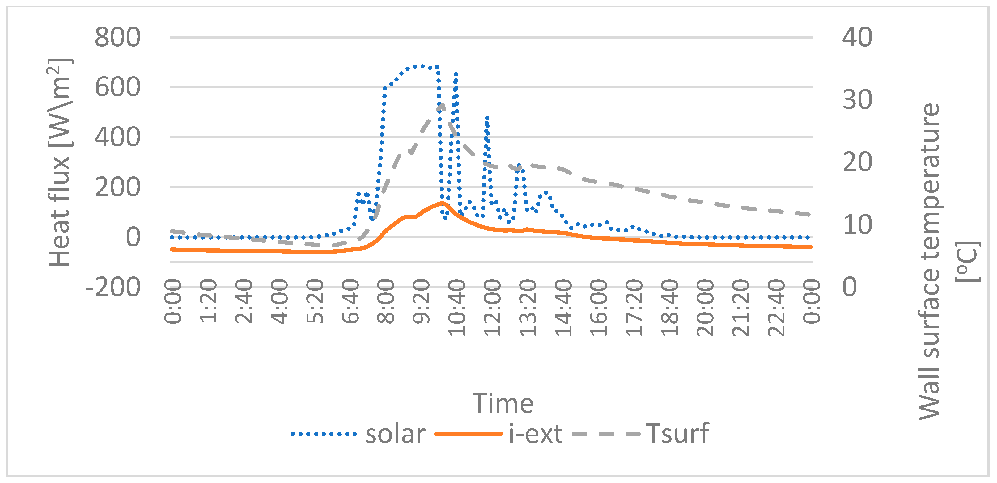
3.6. Solar Energy Absorption

The author’s intention was to investigate the effectiveness of radiation absorption in the summer period. The incident energy cannot be directly calculated from the clear sky model because trees and the building limited its value even on a cloudless day. Unfortunately, due to the lack of data from the sun sensor, the absorption efficiency was presented for 24 April 2021. The energy flowing into the wall was positive during the period of the highest irradiation, which corresponds to the phenomena in the summer. Solar radiation, heat flux on the ext-e surface and external wall surface temperature is shown in Figure 16.

The maximum wall temperature and heat flux show a displacement in relation to the maximum solar radiation as in [33]. The wall temperatures achieved in this study are lower, probably due to the lower absorption of solar radiation.

The heat flux through the control surface ext-e does not exceed one-sixth of the incident radiation flux. The total solar radiation energy was 9144 KJ/m². The energy stored in the wall was calculated as in [14]

$$E_{store}=d_{ext\_mid}{c}_w\rho \left(T_{max,m\_ext\_mid}-T_{min,m\_ext\_mid}\right)=d_{ext\_mid}{c}_w\rho \Delta T_{m\_ext\_mid}$$

(5)

where d_{ext_mid} is the total thickness of the outer and middle layers, c_w specific heat of the wall and ρ density, both values are as in Table 1. The temperature T_{max_m_ext_mid} and T_{min_m_ext_mid} are respectively the lowest and the highest average temperatures of the outer and middle layers considered together. The inner layer of the wall was omitted because its temperature changes slightly and is heated from inside the room and not by solar radiation. The calculated stored energy was 2463 KJ/m², which gives the energy storage efficiency of 27%. The problem of storage efficiency was raised in several studies [6,33]. In work [3], the efficiency of energy storage in a concrete wall was 52%, however, with the incident radiation energy of 16,573 KJ/m². For the summer week of 21–27 June, the stored energy was also calculated according to the Equation (5) and summarised in

Table 4. Energy stored in the wall for the following days of the summer week.

Day	21.06	22.06	23.06	24.06	25.06	26.06	27.06
ΔTm_ext_mid	5.23	5.25	4.31	2.15	1.09	2.38	6.25
Estore [KJ/m2]	3500	3514	2885	1439	730	1593	4183

. As the energy incident in summer is not known, the storage efficiency was not calculated.

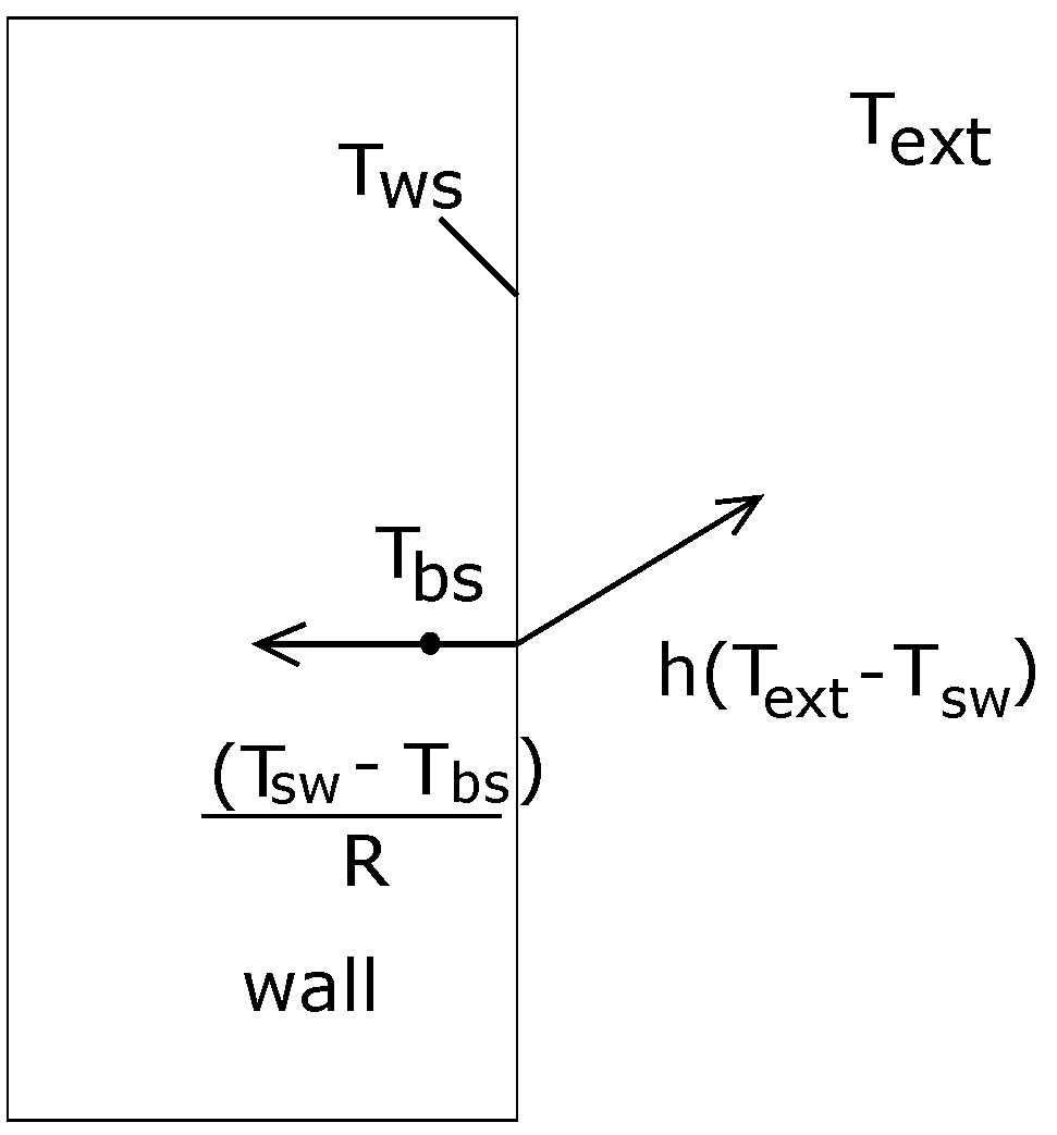
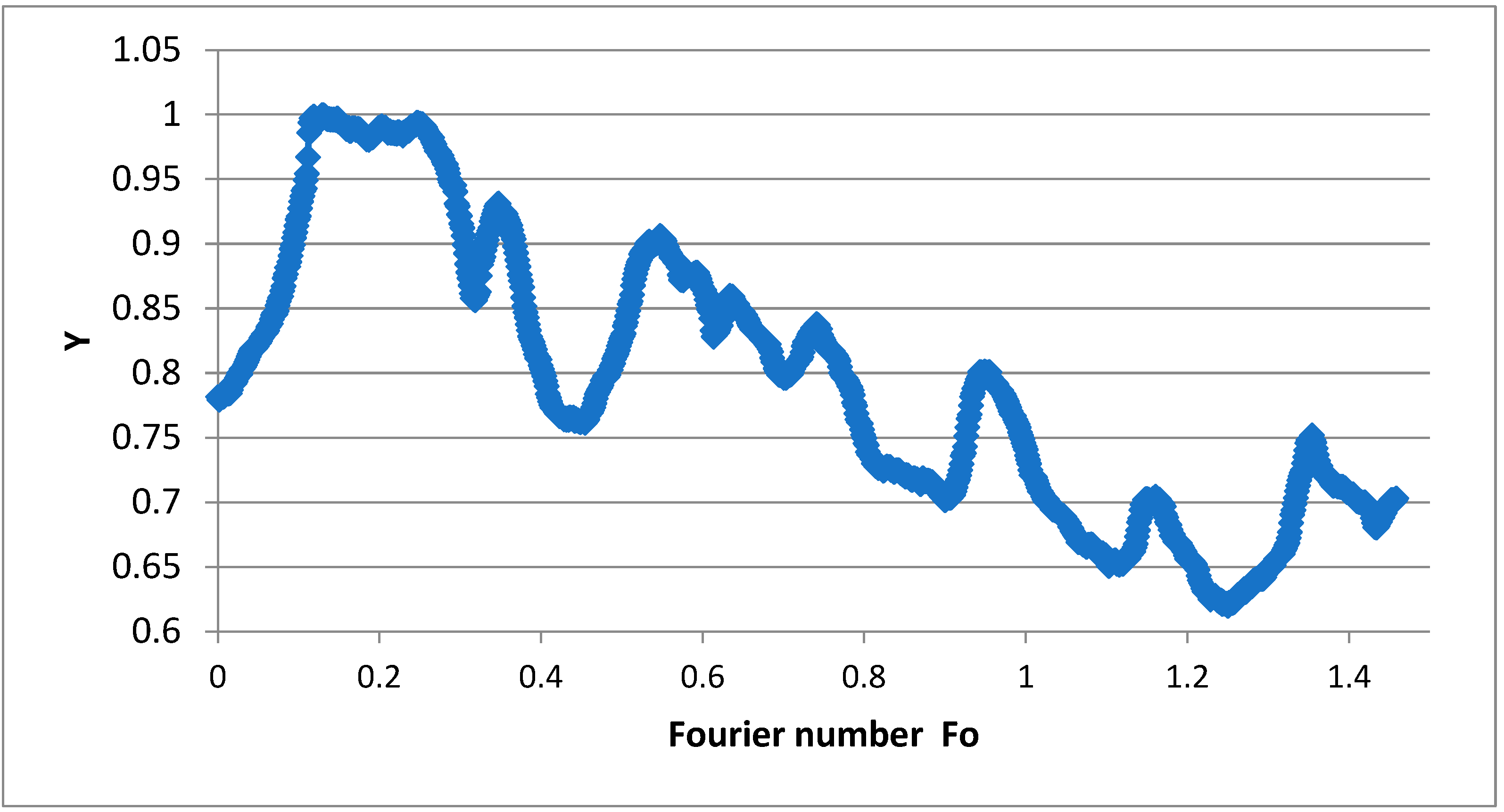
3.7. Heat Transfer Coefficient on External Surface

The heat transfer coefficient can be calculated using energy balance on the wall surface [34]. The heat fluxes on the wall come from convection and longwave radiation, heat transfer by conduction, solar radiation, and sensible heat stored in the wall. In steady-state and night time, the fluxes reduce to conduction and convection along with longwave radiation. Such a situation occurs in winter when the wall temperature changes very little and the solar operation is short. The heat balance is shown in Figure 17.

T_bs denotes temperature below the surface at a certain depth and R is a thermal resistance between the surface and that depth. T_ext is the temperature on the external wall surface and T_ext,a is external ambient temperature. Given the conduction and convection/radiation flux are equal total heat transfer coefficient is calculated from Equation (6)

$$h=\frac{\left(T_{ext}-T_{bs}\right)}{\left(T_{ext,a}-T_{ext}\right)R}$$

(6)

and the Nusselt number

$$Nu=\frac{hl}{{\lambda }_f }$$

(7)

The air movement induced by the wind is parallel to the wall. Because of that boundary layer expands along the width of the detector array and it was assumed as characteristic dimension calculated form Equation (8).

$$l=5c$$

(8)

where c is shown on Figure 1. Heat transfer coefficient according to Equation (6) and Nusselt number form Equation (7) between 4 and 10 January is shown in Figure 18.

The average heat transfer coefficient throughout the calculation period was 8.31 W/(m²K). The minimum value was 6.4 W/(m²K), and the maximum was 17.3 W/(m²K). The maximum peak is due to the sharp rise in ambient temperature. This caused the ambient temperature to come closer to the wall surface temperature, thus reducing the denominator in Equation (6). Apart from this moment, the obtained value of the coefficient is very stable. The Nusselt number calculated for the characteristic dimension from Equation (8) is also shown in Figure 15. The average Biot number was 4.11. The maximum value was 8.58 and the minimum was 3.18. The values above 1 indicate that conduction in the wall is contributing more to heat transfer than convection on the surface. In order to trace the cooling process of the wall surface, a dimensionless temperature was introduced.

$$Y=\frac{T-T_f}{T_0-T_f}$$

where T is the wall surface temperature, T_f is the minimum external air temperature and T₀ is the maximum wall surface temperature in the period under consideration. Therefore dimensionless temperature is defined as the ratio of the maximum excess of the wall surface temperature over the air temperature, to this excess at a given moment in a week.

The values of these parameters for the winter and summer week are presented in

Table 5. Parameters for dimensionless temperature calculation in the given period.

	4–10 January	21–27 June
T0 [oC]	6.76	48.23
Tf [oC]	−1.1	12.8

.

The dependence of Y on the Fourier number for 4–10 January is shown in Figure 19.

The dependence of Y on the Fourier number for 21–27 June is shown in Figure 20.

The variability of the dimensionless temperature over the weekly consideration period was similar both in summer and winter.

4. Discussion

The most dynamic heat exchange occurs in the outer layer. In summer conditions, the highest heat flow was recorded on the outer surface of the wall, while at night the outflow stream with the intensity up to 40 W/m², during the highest solar irradiation, the heat input was 80 W/m². From the inside, heat gains in the room can cause the wall to be heated.

In winter, the net heat flux transferred from the wall to the external environment is so large that solar radiation cannot reverse it. Throughout the day and night, the flow through all control surfaces runs from inside to outside.

Solar radiation energy absorption for an exemplary cloudless day in April was only 27% of the incident value.

The condition of the sky before noon, when the radiation hits the surface of the wall, is essential for the value of the stored energy. The day on 21 June was completely clear, while on 22 June it was cloudy from around 1 p.m. local time. On both of these days, the amount of accumulated energy is similar. According to [35], the amount of energy stored in the wall stabilises after a few days. This conclusion is confirmed in this study, 21 June was the sixth clear day in a row. The energy stored on 21 June and 22 June is very similar. The following days were partly cloudy, 27 June was a sunny day again. There is a visible increase in the difference in daily temperature on that day because the wall was cooled down during the previous days with lower radiation intensity.

The dimensionless temperature during the week has similar values in winter and summer. Taking into account the weekly periods, the wall surface temperature does not drop below 50% of the maximum possible drop when the wall would cool down to the ambient temperature. There are three reasons why the author decided to conduct experimental research on the wall. The steady-state condition as a constant temperature over time is met, but the heat flux is not the same in each layer. This phenomenon can be explained by the non-one-dimensional heat flow in the wall. This is an important conclusion as the steady heat flux condition is widely used to calculate wall temperature. Additionally, the ability to absorb solar radiation by different types of walls is not always known, hence the need for measurements. The third reason why it is worth performing measurement tests is the unknown internal structure of the wall, as it was in this case. When solving energy-related problems of existing buildings, where it is usually difficult to obtain a detailed physical model, experimental approaches could be very useful.

References

1. Foucquier, A.; Robert, S.; Suard, F.; Stéphan, L.; Jay, A. State of the Art in Building Modelling and Energy Performances Prediction: A Review. Renew. Sustain. Energy Rev. 2013, 23, 272–288. [Google Scholar] [CrossRef] [Green Version]
2. PN-EN ISO 52016-1. Energy Performance of Buildings—Energy Needs for Heating and Cooling, Internal Temperatures and Sensible and Latent Heat Loads—Part 1: Calculation Procedures; ISO: Geneva, Switzerland, 2017. [Google Scholar]
3. PN-EN ISO 13786. Thermal Performance of Building Components—Dynamic Thermal Characteristics—Calculation Methods; ISO: Geneva, Switzerland, 2007. [Google Scholar]
4. De Lieto Vollaro, R.; Guattari, C.; Evangelisti, L.; Battista, G.; Carnielo, E.; Gori, P. Building Energy Performance Analysis: A Case Study. Energy Build. 2015, 87, 87–94. [Google Scholar] [CrossRef]
5. Matiasovsky, P. Daily Characteristics of Air Temperature and Solar Irradiation-Input Data for Modelling of Thermal Behaviour of Buildings. Atmos. Environ. 1996, 30, 537–542. [Google Scholar] [CrossRef]
6. Marino, B.M.; Muñoz, N.; Thomas, L.P. Calculation of the External Surface Temperature of a Multi-Layer Wall Considering Solar Radiation Effects. Energy Build. 2018, 174, 452–463. [Google Scholar] [CrossRef]
7. Kontoleon, K.J.; Bikas, D.K. The Effect of South Wall’s Outdoor Absorption Coefficient on Time Lag, Decrement Factor and Temperature Variations. Energy Build. 2007, 39, 1011–1018. [Google Scholar] [CrossRef]
8. Tsilingiris, P.T. On the Transient Thermal Behaviour of Structural Walls—the Combined Effect of Time Varying Solar Radiation and Ambient Temperature. Renew. Energy 2002, 27, 319–336. [Google Scholar] [CrossRef]
9. Dornelles, K.; Roriz, V.; Roriz, M. Determination of the Solar Absorptance of Opaque Surfaces. In Proceedings of the 24th International Conference on Passive and Low Energy Architecture, Singapore, 22–24 November 2007. [Google Scholar] [CrossRef]
10. Berry, R.; Livesley, S.J.; Aye, L. Tree Canopy Shade Impacts on Solar Irradiance Received by Building Walls and Their Surface Temperature. Build. Environ. 2013, 69, 91–100. [Google Scholar] [CrossRef]
11. Becherini, F.; Lucchi, E.; Gandini, A.; Barrasa, M.C.; Troi, A.; Roberti, F.; Sachini, M.; Di Tuccio, M.C.; Arrieta, L.G.; Pockelé, L.; et al. Characterization and Thermal Performance Evaluation of Infrared Reflective Coatings Compatible with Historic Buildings. Build. Environ. 2018, 134, 35–46. [Google Scholar] [CrossRef]
12. Wardziak, Ł.; Jaworski, M. Computer Simulations of Heat Transfer in a Building Integrated Heat Storage Unit Made of PCM Composite. Therm. Sci. Eng. Prog. 2017, 2, 109–118. [Google Scholar] [CrossRef]
13. Kočí, J.; Fořt, J.; Černý, R. Energy Efficiency of Latent Heat Storage Systems in Residential Buildings: Coupled Effects of Wall Assembly and Climatic Conditions. Renew. Sustain. Energy Rev. 2020, 132, 110097. [Google Scholar] [CrossRef]
14. Viegas, G.M.; Jodra, J.I.; San Juan, G.A.; Díscoli, C.A. Heat Storage Wall Made of Concrete and Encapsulated Water Applied to Mass Construction Social Housing in Temperate Climates. Energy Build. 2018, 159, 346–356. [Google Scholar] [CrossRef] [Green Version]
15. Anil Kumar, Y.; Dasha Kumar, K.; Kim, H.-J. Reagents assisted ZnCo2O4 nanomaterial for supercapacitor application. Electrochim. Acta 2020, 330, 135261. [Google Scholar] [CrossRef]
16. Kumar, Y.A.; Sambasivam, S.; Hira, S.A.; Zeb, K.; Uddin, W.; Krishna, T.N.V.; Kumara, K.D.; Obaidatb, I.M.; Kima, H.-J. Boosting the energy density of highly efficient flexible hybrid supercapacitors via selective integration of hierarchical nanostructured energy materials. Electrochim. Acta 2020, 364, 137318. [Google Scholar] [CrossRef]
17. Anil Kumar, Y.; Dasha Kumar, K.; Kim, H.-J. Facile preparation of a highly efficient NiZn2O4–NiO nanoflower composite grown on Ni foam as an advanced battery-type electrode material for high-performance electrochemical supercapacitors. Dalton Trans. 2020, 49, 3622–3629. [Google Scholar] [CrossRef]
18. Yoon, J.H.; Kumar, Y.A.; Sambasivam, S.; Hira, S.A.; Krishna TN, V.; Zeb, K.; Uddine, W.; Kumara, K.D.; Obaidatb, I.M.; Kim, S.; et al. Highly efficient copper-cobalt sulfide nano-reeds array with simplistic fabrication strategy for battery-type supercapacitors. J. Energy Storage 2020, 32, 101988. [Google Scholar] [CrossRef]
19. Owczarek, M. Parametric Study of the Method for Determining the Thermal Diffusivity of Building Walls by Measuring the Temperature Profile. Energy Build. 2019, 203, 109426. [Google Scholar] [CrossRef]
20. Owczarek, M.; Baryłka, A. Estimation of Thermal Diffusivity of Building Elements Based on Temperature Measurement for Periodically Changing Boundary Conditions. Rynek Energii 2019, 5, 76–79. [Google Scholar]
21. Owczarek, M.; Owczarek, S.; Baryłka, A.; Grzebielec, A. Measurement Method of Thermal Diffusivity of the Building Wall for Summer and Winter Seasons in Poland. Energies 2021, 14, 3836. [Google Scholar] [CrossRef]
22. Azhary, K.E.; Raefat, S.; Laaroussi, N.; Garoum, M. Energy Performance and Thermal Proprieties of Three Types of Unfired Clay Bricks. Energy Proced. 2018, 147, 495–502. [Google Scholar] [CrossRef]
23. Sassine, E.; Younsi, Z.; Cherif, Y.; Chauchois, A.; Antczak, E. Experimental Determination of Thermal Properties of Brick Wall for Existing Construction in the North of France. J. Build. Eng. 2017, 14, 15–23. [Google Scholar] [CrossRef]
24. Gourav, K.; Balaji, N.C.; Venkatarama Reddy, B.V.; Mani, M. Studies into Structural and Thermal Properties of Building Envelope Materials. Energy Proced. 2017, 122, 104–108. [Google Scholar] [CrossRef]
25. Marrocchino, E.; Zanelli, C.; Guarini, G.; Dondi, M. Recycling Mining and Construction Wastes as Temper in Clay Bricks. Appl. Clay Sci. 2021, 209, 106152. [Google Scholar] [CrossRef]
26. Akbari, H.; Kurn, D.M.; Bretz, S.E.; Hanford, J.W. Peak Power and Cooling Energy Savings of Shade Trees. Energy Build. 1997, 25, 139–148. [Google Scholar] [CrossRef] [Green Version]
27. Simpson, J.R.; McPherson, E.G. Simulation of Tree Shade Impacts on Residential Energy Use for Space Conditioning in Sacramento. Atmos. Environ. 1998, 32, 69–74. [Google Scholar] [CrossRef]
28. Antonopoulos, K.A.; Vrachopoulos, M. On the Inverse Transient Heat-Transfer Problem in Structural Elements Exposed to Solar Radiation. Renew. Energy 1995, 6, 381–397. [Google Scholar] [CrossRef]
29. Catalina, T.; Virgone, J.; Blanco, E. Development and Validation of Regression Models to Predict Monthly Heating Demand for Residential Buildings. Energy Build. 2008, 40, 1825–1832. [Google Scholar] [CrossRef]
30. Internetowa Stacja Meteo Warszawa. Available online: https://www.meteo.waw.pl/ (accessed on 23 September 2021).
31. Kong, Q.; He, X.; Cao, Y.; Sun, Y.; Chen, K.; Feng, J. Numerical Analysis of the Dynamic Heat Transfer through an External Wall under Different Outside Temperatures. Energy Procedia 2017, 105, 2818–2824. [Google Scholar] [CrossRef]
32. Thomas, L.P.; Marino, B.M.; Muñoz, N. Steady-State and Time-Dependent Heat Fluxes through Building Envelope Walls: A Quantitative Analysis to Determine Their Relative Significance All Year Round. J. Build. Eng. 2020, 29, 101122. [Google Scholar] [CrossRef]
33. Dhifaoui, B.; Ben Jabrallah, S.; Belghith, A.; Corriou, J.P. Experimental Study of the Dynamic Behaviour of a Porous Medium Submitted to a Wall Heat Flux in View of Thermal Energy Storage by Sensible Heat. Int. J. Sci. 2007, 46, 1056–1063. [Google Scholar] [CrossRef]
34. Jayamaha, S.; Wijeysundera, N.; Chou, S. Measurement of the heat transfer coefficient for walls. Build. Environ. 1996, 31, 399–407. [Google Scholar] [CrossRef]
35. Li, H.; Zhong, K.; Yu, J.; Kang, Y.; Zhai, Z. Solar Energy Absorption Effect of Buildings in Hot Summer and Cold Winter Climate Zone, China. Sol. Energy 2020, 198, 519–528. [Google Scholar] [CrossRef]
Figure 1. Arrangement of temperature sensors in the wall.
Energies 14 08093 g001
Figure 2. Microscopic photos of a brick sample from the tested wall.
Energies 14 08093 g002
Figure 3. View of the tested wall and field of view of the solar radiation sensor.
Energies 14 08093 g003
Figure 4. Regular temperature grid generated after the recorded field approximation.
Energies 14 08093 g004
Figure 5. Air temperature and solar radiation on horizontal surface for (a) 4–10 January, (b) 21–27 June 2021 for Warsaw [30].
Energies 14 08093 g005
Figure 6. Heat fluxes in the considered wall.
Energies 14 08093 g006
Figure 7. Temperature differences S4D-S4 and S4U-S4 indicating vertical heat flow in wall on 23–30 January 2020.
Energies 14 08093 g007
Figure 8. Temperature differences S4D-S4 and S4U-S4 indicating vertical heat flow in wall on 21–27 June 2020.
Energies 14 08093 g008
Figure 9. Recorded temperatures in the wall for winter week.
Energies 14 08093 g009
Figure 10. Recorded temperatures in the wall for summer week.
Energies 14 08093 g010
Figure 11. Graph of the average temperature in three layers of the wall on 22 June 2021.
Energies 14 08093 g011
Figure 12. Graph of the average temperature in three layers of the wall on 5 January 2021.
Energies 14 08093 g012
Figure 13. Fluxes of heat between the layers, the direction of the arrows indicates a positive value.
Energies 14 08093 g013
Figure 14. Heat fluxes between the layers on 27 June 2021.
Energies 14 08093 g014
Figure 15. Heat fluxes between the layers on 8 January 2021.
Energies 14 08093 g015
Figure 16. Solar radiation, heat flux on the ext-e surface and external wall surface temperature on 24 April 2021.
Energies 14 08093 g016
Figure 17. Energy balance on the outside surface of wall in steady-state.
Energies 14 08093 g017
Figure 18. Heat transfer coefficient and Nusselt number on outer surface of the wall 4–10 January.
Energies 14 08093 g018
Figure 19. Dimensionless temperature as a function of Fourier number for 4–10 January.
Energies 14 08093 g019
Figure 20. Dimensionless temperature as a function of Fourier number for 21–27 June.
Energies 14 08093 g020