Abstract
In this work, a data-driven methodology for modeling combustion kinetics, Learned Intelligent Tabulation (LIT), is presented. LIT aims to accelerate the tabulation of combustion mechanisms via machine learning algorithms such as Deep Neural Networks (DNNs). The high-dimensional composition space is sampled from high-fidelity simulations covering a wide range of initial conditions to train these DNNs. The input data are clustered into subspaces, while each subspace is trained with a DNN regression model targeted to a particular part of the high-dimensional composition space. This localized approach has proven to be more tractable than having a global ANN regression model, which fails to generalize across various composition spaces. The clustering is performed using an unsupervised method, Self-Organizing Map (SOM), which automatically subdivides the space. A dense network comprised of fully connected layers is considered for the regression model, while the network hyper parameters are optimized using Bayesian optimization. A nonlinear transformation of the parameters is used to improve sensitivity to minor species and enhance the prediction of ignition delay. The LIT method is employed to model the chemistry kinetics of zero-dimensional and -air combustion. The data-driven method achieves good agreement with the benchmark method while being cheaper in terms of computational cost. LIT is naturally extensible to different combustion models such as flamelet and PDF transport models.
1. Introduction
Although the simulation of high Reynolds number combusting flow includes several computationally expensive elements, including turbulent feature prediction, the modeling of chemical kinetics is the main bottleneck. Numerical integration of reaction mechanisms mathematically must contend with an extremely stiff system of ordinary differential equations (ODEs). The stiffness of the equations is represented by the range of eigenvalues, spanning nine orders of magnitude. The difficulties caused by the stiffness are compounded by the size of the system. The number of differential equations scales with the number of chemical species, which can reach into the hundreds for complex hydrocarbon fuels. The chemical kinetics of real applications, such as n-heptane combustion, comprises more than 100 species and 1000 reactions. Furthermore, the chemical time-scale O() is much smaller than the smallest flow time scale for most engines, O(), which makes the computation very expensive.
There have been efforts to reduce the cost of kinetics by developing reduced mechanisms and chemistry tabulation techniques. As a detailed chemical kinetic mechanism with a large size and chemical stiffness restricts the computation of real combustion applications, it is inevitable to reduce the detailed mechanism to a smaller number of reactions. There are two levels of mechanism reduction: The first level is the elimination of insignificant reactions and species (skeletal reduction) using methods such as Directed Relation Graph (DRG) [1], Rate-Controlled Constrained Equilibrium (RCCE) [2,3], and Path Flux Analysis (PFA) [4]. The second level is the consideration of the impact of timescales on the whole reaction system (global reduction) methods such as Computational Singular Perturbation (CSP) [5,6], and Intrinsic Low Dimensional Manifold (ILDM) [7]. However, reduced mechanisms result in a less reliable description of chemistry, and the level of reduction is a large challenge [8]. The tabulated chemistry technique computes a chemical mechanism with an affordable computational cost. In this approach, the chemical kinetics are solved with the interpolation of precomputed and stored values [9], which results in the reduction of real-time chemistry computation. In the in Situ Adaptive Tabulation (ISAT), the thermochemical solution can be tabulated in real-time simulation and reused in later sequences of the simulation [10,11]. The performance of the tabulation techniques strongly depends on the application as the accuracy and efficiency drop for complex turbulent combustion.
Recently, machine learning has shown promise for assisting combustion simulation. For instance, Yap et al. used Artificial Neural Networks (ANN) to control and optimize exhaust emissions [12]. Zamaniyan and his colleagues applied an ANN to model an industrial hydrogen plant [13]. There have been many efforts to use machine learning models, such as deep neural networks [14], convolutional neural networks [15], and generative adversarial networks [16] to predict sub-scale combustion features in turbulent combustion simulations. Owoyele et al. [17] studied the effect of bifurcating turbulent combustion inputs to improve regression tasks among specialized artificial neural networks. In addition, combustion researchers have introduced several data-driven tabulation methods to accelerate chemical kinetics computation. Christo et al. [18], for their first attempt, employed a deep neural network to model a 4-step H2–CO2 chemical mechanism in a simulation of turbulent flame. Subsequently, Blasco et al. [19,20] applied an ANN to a reduced methane combustion mechanism including four steps and eight species. Later, they observed that it is extremely difficult to have one network modeling a complex multidimensional combustion mechanism, and expanded the method by clustering the composition space [21]. In this way, the thermochemical space is divided into multiple subspaces with a Self-Organizing Map (SOM) to have a dedicated regression network for each subspace. They applied the SOM-MLP (multilayer perceptron) method to a reduced methane combustion application with five steps. They reported good agreement with the benchmark and savings in computational time and memory usage. In the recent decade, Chatzopoulos and Rigopoulos [22] introduced an ANN model for a RCCE-reduced CH4 mechanism trained with abstract non-premixed flamelets. Furthermore, Franke et al. [23] proposed an ANN model coupled with RCCE and CSP reduction methods to simulate the LES-PDF Sydney flame. They used an abstract problem to generate the ground-truth data. Most recently, An et al. [24] applied a similar method, called SOM-BPNN (Back-Propagation Neural Network), to model the combustion chemistry of hydrogen/hydrocarbon-fueled supersonic engines. Also, Owoyele and Pal [25] introduced a different data-driven tabulation method using a neural ODE approach, in which they have one network for each species of a H2–O2 combustion.
In this work, the goal is to replace the integration of stiff chemical ODEs with a relatively fast machine learning scheme called Learned Intelligent Tabulation (LIT). We use a family of networks that self-selects during the progression through reactions. The selection process is based on unsupervised clustering as a preprocessing step using a map that is produced during training. Each network is trained using a subset of ground truth data appropriate to the local temperature and composition regime. Because chemical species concentrations span at least nine orders of magnitude and are not equally important, a nonlinear transformation of the primitive variables is used in training the network and calculating the loss function. The final algorithm is tested in a multi-dimensional CFD code. The results include the construction, accuracy, and speed-up assessments of this approach.
While there have been works in the literature to model hydrogen combustion, the LIT method captures the full hydrogen mechanism without any reduction. All species are modeled with the networks. Validation tests include the 0D kinetics test which directly evaluates the performance of the kinetics solver, without the consideration of flow dynamics such as convection and diffusion. There have been studies such as Franke et al. and Chatzopoulos et al. who applied a similar method to tabulate kinetics of CH4 combustion along with rate-controlled constrained equilibrium to reduce the full mechanism. However, for such extensive mechanisms LIT allows regression with a subset of species chosen at the user’s convenience and adds heat release to the output vector to correct for the effect of neglected species. This novel approach makes LIT capable of matching the full mechanism in terms of energy solution prediction. We report on a method of decoupling the time step of the time integration with the output of the ground truth data to allow arbitrary augmentation of the training data without interpolation. Furthermore, LIT utilizes nonlinear transformation of species concentration and Bayesian optimization techniques, which substantially improve the accuracy of the method to capture the chemistry dynamics.
This article is organized as follows. Section 2 includes the detailed description of the LIT method. The workflow and challenges are explained, which involves data generation, input clustering, DNN regression, and the integration of networks into a CFD solver. Next, Section 3 presents the validation cases, including hydrogen–oxygen and methane–air combustion. Results of LIT method are compared with several benchmarks.
2. Methodology
A reacting flow solver includes the computation of chemical species transport equations added to the fluid flow equations such as mass, momentum, and energy conservation. The conservation of species mass fraction is formulated as
where t represents time, is mixture density, is velocity, p is pressure, is the mass fraction of species i, is the diffusion velocity of species i, and is the mass reaction rate of species i. The CFD solver computes the discretized transport equations using the finite volume method, for which the chemical source terms are required. It is noteworthy that the calculation of the reaction rates could consume up to of the total computation in a reacting flow depending on the complexity of the reaction mechanism [10]. The reaction rate of species from all chemical reactions is formulated as
where is the rate of change of species i by the jth reaction in mole concentration and is the molecular weight of the ith species. The rates of concentration change are described as , which is calculated over the flow time-step after solving the system of differential equations representing the chemical reactions. In general, chemical reactions are described by a system of first-order ODEs, which can be represented as
where is the thermochemical composition vector including temperature T, pressure P and the vector of species mole fractions, and S represents the chemical reactions based on the Law of Mass Action [26]. The CFD solver loops over all the computational cells to construct and integrate the reaction ODE system. Different reactions work at different rates and time scales, which makes the system mathematically stiff and computationally expensive. Our approach is to regress this stiff system using a more expedient DNN.
One of the most common applications of DNN is regression of nonlinear problems. Given that a well-generated data set is available for learning, a DNN can fit a function to model the hidden physics [27]. This capability of the DNN is utilized in this work to model the chemical kinetics and replace the ODE solver in the simulation workflow. To achieve this goal, we developed the LIT method, that is described in the following sections. The workflow of LIT is comprised of four steps, as illustrated in Figure 1.
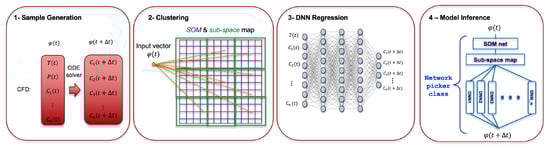
Figure 1.
The overview of the Learned Intelligent Tabulation (LIT) method involving the use of unsupervised learning to reduce dimensionality of the data (Step 2), performing DNN regression task on each reduced compositional space (Step 3) and finally, model inference coupled to a CFD code (Step 4).
- LIT starts with ground-truth generation from the reference ODE solver. Performance of the trained DNNs strongly depends on the quality of the training data and similarity of the data to the objective problem. To augment the data, we have used smaller time steps in sampling the data. As the solution time step is fixed in our validation case, the generated samples are paired according to the required solution time step. The last step in data preprocessing is data scaling to make inputs more distinguishable to the networks.
- Clustering is the second step after generation and preprocessing the training data. As kinetics are such a multidimensional and multiscale problem, it is very difficult for one DNN to cover the entire combustion space. It requires a very deep and wide network to approximate the entire dynamics and leads to higher computational costs. As a result, dividing the effort among multiple DNNs improves the accuracy and lowers the cost as well. After clustering the samples into self-organizing map (SOM) bins [28], the data are mapped to a subspace grid. Each subspace includes several SOM bins.
- Functional mapping from input features to target vector is implemented utilizing regression DNNs for each subspace. In this work, fully connected (Dense) neural networks are used to find the functional mapping between the target to the input features. In addition, Bayesian Optimization [29] is employed to find the optimum hyper-parameters.
- After training the SOM network and DNNs for each subspace, C++ codes are automatically created for all networks, which are integrated with the CFD solver through an inference code. The inference is designed to be scaled to as many DNNs as required using object-oriented programming. Details of each step are described in the following sections.
2.1. Ground-Truth Data Generation
Generation of training data is a critical step in the learning of combustion kinetics. The data should be structured based on the problem definition . For a chemical reaction, the function to approximate is the kinetics ODE system in Equation (3). Therefore, the input vector is the thermochemical state at time t, , and the output vector is the thermochemical composition at without temperature and pressure which are not direct outputs of the chemical reactions: . Note that the time step size can be added to the input vector as been done in the literature [20], however it is not considered in this work since all validation cases are simulated with a fixed time step.
We used the chemFoam solver from the OpenFOAM 5.0 framework [30], which is an open-source CFD software package implemented in C++. OpenFOAM has an extensive range of computational applications including chemical reactions and combustion. chemFoam is a zero-dimensional solver for chemical reaction and is utilized in this study to generate the ground-truth data. Samples are created for a variety of initial conditions and simulation parameters to produce comprehensive training data.
Supervised data-driven models are being successfully used for a wide range of complex applications. However, these models are known to be very data-hungry, and their performance relies strongly on the size and quality of the training data. Therefore, it is critical to create a large dataset where the solution is decoupled from the actually used in the ground truth generation. In this work, we augment the data by running the ground-truth simulation with relatively smaller time steps and pairing the data samples according to a coarser solution time step. The actual ground truth controls how many data points are produced, and the interval for pairing controls the solution used for training. The apparent corresponds the to the time step anticipated in the CFD calculation. In this way, we can generate as much data as our training needs. For instance, the solution time step of the combustion is s, while the data were generated with . The generated data are then preprocessed to match the solution time step. In more detail, each input vector is paired with the correct output according to the solution time step.
Primitive species concentrations represent a very challenging quantity for training neural networks, because the change in minor species concentrations is happening over very small values. The network cannot react to changes of species concentration of such small values as they are practically noise compared to the major species. Therefore, we used a 6th root transformation that makes the small changes more visible for a neural network. This helps the network to capture those critical changes. As is illustrated for a major species and minor species H in Figure 2, primitive values are unable to show small changes of concentration, which are crucial for the network to learn the ignition delay. However, the changes throughout the combustion process are more detectable with the 6th root species concentrations. Different transformations were explored and the 6th root offered the best trade-off between minor species sensitivity and robust representation of major species. Log transformations were found to be too heavily biased in favor of minor species fidelity at the expense of major species.
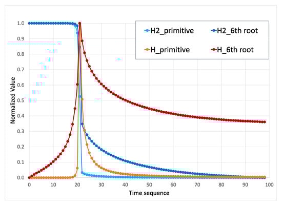
Figure 2.
Illustration of different nonlinear transformations on a major and minor species. The 6th root transformation allows the low concentrations of both to be visible to the networks.
The last step in data preprocessing is the normalization of input and output parameters. Rarely, neural networks are applied directly to the raw data without normalization. Generally, we need preparation to help the network optimization process and maximize the probability of obtaining good results. Normalizing the input and output vectors consists of mapping the data to the vector norms. Typically, data are linearly transformed to [0, 1] or [−1, 1]. The max and min values of the vectors would be required in building the integration network. The normalization step prevents networks from facing inputs with different scale and distribution. In this work, the input and output vectors are linearly scaled to [0, 1].
2.2. Composition Space Clustering
The chemical system presents a complex multidimensional problem, and covering the whole dynamics with a single neural network would be quite challenging. Therefore, it is pragmatic to divide the task among several networks. To achieve this subdivision, a clustering step is added to the LIT method. In addition, the data clustering means that a smaller network with less computational cost can be used for each individual cell. As the cost of querying clustering networks is very small compared to the inference cost of DNNs, the overall computational cost drops significantly.
A self-organizing map [28] is employed to cluster the combustion composition set. SOM is an unsupervised learning technique that identifies groups of similar data. The groups are organized in a one or two-dimensional map. Different map topologies are available such as a grid, hexagonal, or random topology to arrange the clusters. One neuron is assigned to each cluster, and the Euclidian distance in the composition space is the clustering criterion. New samples are clustered into the most similar neuron with the shortest Euclidean distance [28]. In this way, SOM learns both the distribution and topology of the input composition space. The self-organizing feature map (SOFM) from the Matlab learning toolbox [31] is employed in this work for clustering.
After the SOM training is completed, the dataset is clustered into the SOM map, which would be the reference to divide the thermochemical samples. One could train one regression DNN for each SOM neuron, however, some SOM neurons do not contain enough data to train a DNN. Therefore, the SOM map is projected into a subspace map, and a DNN is trained for each subspace. An example of evolution clustered into the SOM map and converted into a subspace map is depicted in Figure 3 (left). Furthermore, the temperature plot of the subspace data is shown in Figure 3 (right). As is shown, the unsupervised composition space clustering divides the combustion dynamics into different phases. As a consequence, we can train one DNN for each phase of the solution.
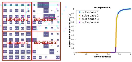
Figure 3.
SOM clustering map converted into subspace map (left) and temperature plot of subspace clusters (right).
2.3. Regression Network
DNNs are capable of modeling complex nonlinear systems. The depth and width of the network architecture can be adjusted depending on the difficulty of the problem. The first layer is the input layer with the same number of neurons as the size of input vector. The output layer also has the same size as the output vector, which is the concentration of species. Several fully connected layers (hidden layers) with many neurons are considered between the input and output layers. All neurons in each layer are connected to the neurons of the neighboring layers. Each neuron calculates the weighted summation of inputs from previous layer and applies a non-linear activation function as
where is the output from fully connected layer, is nonlinear activation function, is the input from previous layer, W is weight, and b is bias of the neuron. In the DNN training, weight and bias values are learned and stored. We have used the Matlab Deep Learning toolbox [31] to perform the training. While the neural network implementation is fairly straightforward, the a-priori estimation of the best network hyperparameters, and the architecture itself is nontrivial due to the multiscale, non-local, and nonlinear nature of the dataset. To discover the best performing settings for our dataset, an Automatic Machine Learning (autoML) strategy is used. Among the many available optimization methods in the literature [32], we employed the Bayesian Optimization (BayesOpt) approach, which has shown good performance for other data-driven tasks ([29,33]).
The learning process for a ML algorithm such as neural networks is often stochastic in nature. This is due to the nature of the optimization solver and the loss manifold. The loss landscape/manifold for these multivariate time series problems such as in chemical kinetics are non-convex, and high-dimensional. That implies the choice of the hyperparameters used in the learning process and the design/architecture of the network has a leading order impact on the expected error and associated uncertainties of the model. In this study, we use an automatic Machine Learning (autoML) paradigm to choose optimum network hyperparameters and automate the network design process, previously introduced in [34]. The autoML uses Bayesian Optimization (BayesOpt) to navigate the range of parameters to find optimal solutions. In this study, the learning algorithm is modeled as a sample from Gaussian Process (GP). The posterior distribution induced by the GP leads to efficient use of information gathered by previous experiments, enabling optimal choices for what parameters to try next. Table 1 shows the optimization matrix, the range of each parameter and the corresponding interpolation strategies. The autoML was run for up to 100 function evaluations and the loss function was defined as the performance of the trained network on the validation dataset. Each evaluation included a network training of up to 40 epochs. At the end of training, the loss on validation dataset was stored and only the top five performing networks were retained to save disk space.

Table 1.
Optimization matrix with interpolation strategies and range of investigation for each hyperparameter.
In addition, the network architecture itself is optimized. This is done by using the network width (number of layers) and depth (number of neurons in each layer) a parameter to optimize using the BayesOpt method. The depth and width are implemented as a series of repeating network blocks: fully connected layer->activation function. The solver used in all these studies is the ADAM optimizer [35].
To save time and reduce complexity of integrating different sized networks, this autoML step was carried out once for the entire dataset and the best design was chosen and re-implemented subsequently for each of the sub-spaces. The assumption was that the subspace loss manifolds are represented in the overall loss landspace and therefore a global optimization, might hold for locally smaller subspaces.
2.4. Network Model Integration
After completing the training of the SOM network and DNNs, the networks must be integrated with the CFD solver. As we are using OpenFOAM, which is implemented in C++, the trained networks are converted into C++ code for integration. To achieve this, we used a Matlab Coder tool to generate C++ code of the DNNs and SOM network along with the weight and bias binary files.
Networks are integrated into the CFD solver as a C++ library. The base class contains one SOM network and a large number of DNNs. It initializes the networks with its constructor where the weight and bias values of all layers are read from the disk. For each input, the class calls the appropriate DNN based on the SOM’s response and calculates the output. The inference code receives species concentration , temperature T, and pressure P, and calculates the outputs . Pseudocode of the inference is illustrated in Algorithm 1.
| Algorithm 1 LIT inference pseudocode |
| 1: Networks Initialization 2: for do 3: for do 4: 5: 6: Prediction for each input Input: 7: 8: 9: SOM’s response 10: 11: DNN’s prediction 12: 13: 14: Output: |
3. Results and Discussion
To validate LIT, we start with a zero-dimensional reactor at constant pressure. For the hydrogen kinetics, all species are regressed using LIT without any simplification. Next, a methane–oxygen reactor is modeled, where the GRI 3.0 mechanism with 53 species is utilized for ground truth generation.
With 53 species, the methane state space is very highly dimensional, and regressing all species is very challenging. Therefore, we employed a reduced parameter space that includes five species. The selection of these five species is inspired by a one-step methane-oxygen global reaction. For both validation tests, LIT’s prediction is compared with OpenFOAM ODE solver, and the gained speedup is reported.
3.1. Hydrogen-Oxygen Combustion
The first test for LIT is a zero-dimensional reactor, which has no convection or diffusion, and the chemical kinetics is the only factor in species evolution. Therefore, this problem is an appropriate first test to evaluate the performance of LIT method. In this work, a hydrogen–oxygen reaction is considered at various initial temperatures and equivalence ratios , while the pressure is fixed at . The ground truth comes from a detailed mechanism with 10 species, namely, and 27 reactions. The training data generated for this problem include the simulation results of the reactor from initial conditions to a post-reaction final state. The initial condition is altered to vary the equivalence ratio –1.5 and initial temperature in the range of 1000–1200 K. Data are generated with a smaller time step s to augment the training data as was explained in Section 2, while the objective simulation time step is . The input vector involves the temperature and concentration of all species , and the output of the network is the concentration of all species . All species including major and minor species are modeled in this work. Temperature is not used as an output because species enthalpies can be used for calculating the energy release.
The LIT configuration for this problem involves a SOM map, which is projected to a subspace map. Therefore, combustion is divided into 16 regression DNNs to model. The dimensions of the SOM map and the required number of subspaces can be different for different problems. Franke et al. [23] and An et al. [24] studied the effect of SOM map configuration on the accuracy of the model. For DNN regression, we have a fully connected network with three dense layers having and 25 hidden neurons, respectively.
Figure 4 compares the solution from the LIT method to the result from the OpenFOAM ODE solver, which solves the complete chemistry mechanism. The figure shows the results for two equivalence ratios of and , while initial temperature is fixed K. The plots on the left show normalized temperature and reactants’ mass fraction. The middle plots and plots on the right are the normalized mass fraction of and H, and of and . In all plots, the ODE solver solution is plotted with lines, while LIT results are represented by symbols. According to Figure 4, LIT correctly predicts the combustion behavior for both lean and rich conditions. Prediction of temperature and reactants is in good agreement with the benchmark. Comparing different species, LIT’s prediction of major species with monotonic growth including and is more accurate than the minor species such as and .
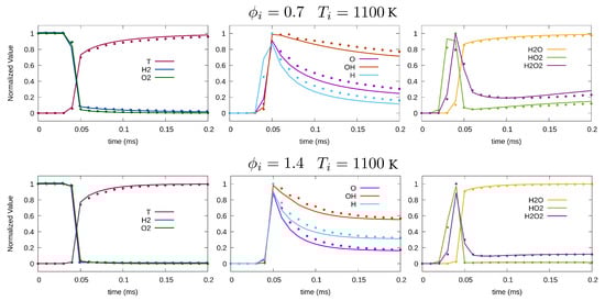
Figure 4.
Temporal variation of normalized temperature and species concentration for K, (top), and (bottom). Solid line and symbols represent the OpenFOAM and LIT solution, respectively.
Figure 5 plots the temporal evolution of species mass fraction at various initial temperatures K and 1150 K, while the equivalence ratio is set at . Overall, LIT shows good accuracy in the prediction of chemical evolution for both cases. Higher temperature with faster reaction appears to be more challenging for the method. Minor species with non-monotonic dynamics such as and proved to be relatively more difficult to capture for the DNN.
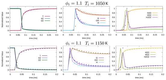
Figure 5.
Temporal variation of normalized temperature and species mass fraction for , K (top), and K (bottom). Solid line and symbols represent OpenFOAM and LIT solution, respectively.
Machine learning methods are known to perform well for points from the middle of the training space because of data interpolation. Consequently, a more difficult test of LIT will occur at the boundaries of the training space, where K and 1200 K, and and . Figure 6 shows the results for these edge cases, where the line plots of temporal evolution of chemical species and temperature are presented. LIT performs well at the edge of equivalence ratio range, though the results show slightly more error at the extreme temperatures. As expected, minor species tend to show more error compared to the middle of the training space, while the tendency of major species at K is to slightly lag the ground truth.
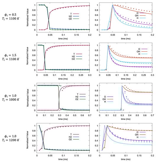
Figure 6.
Temporal variation of normalized temperature and species mass fraction at the boundaries of dataset. Solid line and symbols represent OpenFOAM and LIT solution, respectively.
Figure 7 shows the estimation of ignition delay time versus equivalence ratio. Results of the full mechanism are represented by a line, and LIT results are depicted by square symbols. Ignition delay time is the time needed for a mixture of fuel and oxidizer to react and reach to the maximum rate of temperature rise. This parameter provides a benchmark of the overall behavior of a combustion. Equivalence ratio varies from lean to rich , while initial temperature varies from K to K. Overall, LIT shows good agreement with the OpenFOAM solution.
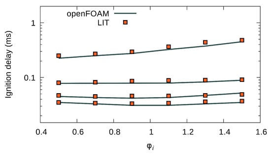
Figure 7.
Ignition delay of combustion as a function of for different –1150 K.
3.2. Methane–Oxygen Combustion
The ultimate goal is to extend the LIT method to more complex fuels. Methane, a very simple hydrocarbon fuel, has a much more complicated parameter space. If we use the size and complexity of GRI 3.0 as an indicator, the methane combustion mechanism is represented by 53 species and 325 reactions [36]. The number of reactions is only relevant for generating the ground truth data, but the number of species raises an important question: how many should be represented in the LIT parameter space? To use all 53 would incur the “curse of dimensionality”, where the large number of dimensions demands an impossible amount of training data. Various sizes of parameter vectors were considered, but ultimately a small size of five species worked best including , and . These species were chosen largely based on their appearance in the one step global mechanism .
The ground truth data are generated from GRI 3.0, which provides the evolution of all 53 species concentrations, though only the subset of the five species and the total generated heat from the reactions are stored for training. The initial temperature is K, and equivalence ratio is for this training and test. The input vector includes temperature and concentration of the five species , and the output vector includes concentrations of species and total heat source . The heat source is required as the mechanism is simplified.
The LIT configuration for combustion involves a SOM map, which is projected to a subspace map. As a result, the combustion dynamics are divided into 25 regression DNNs. For DNN regression, we have a fully connected network with 5 dense layers having , and 25 hidden neurons, respectively. After the training, the accuracy of the networks is evaluated with the test data, which is of the ground truth data. The mean and standard deviation of absolute error of normalized values are plotted in Figure 8. The networks deliver good accuracy in prediction of output quantities.
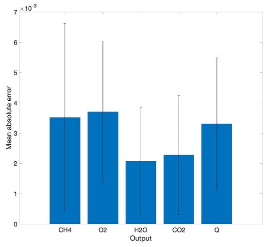
Figure 8.
Mean absolute error of LIT prediction compared to OpenFOAM data. Normalized output quantities [0–1] are used in this plot. Standard deviation of error is plotted too.
Figure 9 compares the solution from the LIT method to the result from the ODE integrator, which solves the complete GRI 3.0 mechanism. The plot on the left shows the temperature variation. The middle plots are the mass fraction of and , and plots on the right are the mass fraction of and . In all plots, the ODE solver solution is plotted with lines, while LIT results are represented by symbols. According to the results, LIT correctly predicts the temperature and concentrations compared to the benchmark. Overall, LIT shows good agreement with the ODE solution.
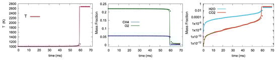
Figure 9.
Temporal variation of temperature and species mass fraction. Solid line and symbols represent the OpenFOAM and LIT solutions respectively.
3.3. Speedup
Ultimately, the motivation for using the machine-learning surrogate instead of the ODEs is to provide faster results. To assess the value of the present approach, we measured the speedup between using the system of ODEs and LIT. The speedup was defined as the ratio of the ODE computational cost divided by the LIT computational cost. The assessment was performed for both hydrogen and methane reactions and is shown in Figure 10.
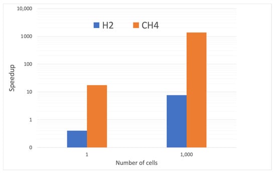
Figure 10.
Observed speedup from applying LIT for and combustion with reference to the OpenFOAM ODE solver.
The results show tests with both a single computational cell and with a set of one-thousand cells. The computational cost of LIT does not include time for reading the networks from the disk and allocating memory for each network, which occurs once before the solution loop starts. When applied to a single computational cell for hydrogen, the speedup is less than unity, indicating that LIT is slower than using an ODE. The main reason is that hydrogen is such a cheap mechanism with small number of reactions. Because of the extent of the GRI 3.0 mechanism, the single computational cell still benefits from the use of LIT with a roughly twenty-fold speedup.
Once the networks are instantiated, they can be used repeatedly for inference within a CFD code. The right data pair in Figure 10 shows a more realistic scenario where the LIT scheme is applied to a batch of one thousand cells. The start-up cost of LIT is now amortized over one thousand executions, providing a much more efficient deployment. The speedup with the relatively simple hydrogen chemistry is roughly eight while the speedup with the methane chemistry is over one-thousand. Because CFD simulations are expected to have on the order of one million cells, the speedup with one thousand cells probably underestimates the speedup expected in actual use.
4. Conclusions
In this work, we introduced a machine learning method to tabulate chemical kinetics. It was found that a two-step process provided an expedient method for regressing hydrogen/oxygen combustion. An examination of the self-organizing map showed that individual nodes of the SOM could be data-poor, and that a grouping process provided a balance between the data requirements and the fidelity gain offered by using numerous networks.
An essential part of the process was the use of a nonlinear transform so that the lower concentrations of species were still visible to the networks despite their small magnitude. Various transformations were investigated and a one-sixth root was found to give a good balance of low-concentration response and high-concentration fidelity. This transformation proved essential for accurate prediction of ignition delay.
When applied to a relatively simple reaction system, such as hydrogen/oxygen combustion, the parameter space used in the regression could include the full complement of species. However, it was found that with a much more complex system, methane, a reduced set of species offered good fidelity at low cost. Speedup for this system was found to exceed one-thousand.
Natural next steps for this work would be further testing over a wide range of conditions for methane and extension to complex hydrocarbons, such as n-heptane. The present results for methane represent only a single initial condition. If these extensions are found to be successful, the LIT approach will dramatically accelerate the CFD simulation of combusting flows.
Author Contributions
Conceptualization, M.H. and D.P.S.; Validation M.H.; Investigation, P.M.; Software, M.H. and N.D.S.; Supervision, D.P.S. All authors have read and agreed to the published version of the manuscript.
Funding
The authors from the University of Massachusetts Amherst received funding from the ICEnet consortium, including MathWorks, NVIDIA Corp. AVL, Convergent Science, SIEMENS/CD-Adapco and Cummins Inc.
Institutional Review Board Statement
Not applicable.
Informed Consent Statement
Not applicable.
Data Availability Statement
Not applicable.
Acknowledgments
The authors from the University of Massachusetts Amherst would like to acknowledge the support of the ICEnet consortium, including MathWorks, NVIDIA Corp. AVL, Convergent Science, SIEMENS/CD-Adapco and Cummins Inc.
Conflicts of Interest
The authors declare no conflict of interest.
References
- Lu, T.; Law, C.K. Toward accommodating realistic fuel chemistry in large-scale computations. Prog. Energy Combust. Sci. 2009, 35, 192–215. [Google Scholar] [CrossRef]
- Jones, W.; Rigopoulos, S. Rate-controlled constrained equilibrium: Formulation and application to nonpremixed laminar flames. Combust. Flame 2005, 142, 223–234. [Google Scholar] [CrossRef]
- Jones, W.; Rigopoulos, S. Reduced chemistry for hydrogen and methanol premixed flames via RCCE. Combust. Theory Model. 2007, 11, 755–780. [Google Scholar] [CrossRef]
- Sun, W.; Chen, Z.; Gou, X.; Ju, Y. A path flux analysis method for the reduction of detailed chemical kinetic mechanisms. Combust. Flame 2010, 157, 1298–1307. [Google Scholar] [CrossRef]
- Valorani, M.; Creta, F.; Goussis, D.A.; Lee, J.C.; Najm, H.N. An automatic procedure for the simplification of chemical kinetic mechanisms based on CSP. Combust. Flame 2006, 146, 29–51. [Google Scholar] [CrossRef]
- Lam, S. Using CSP to understand complex chemical kinetics. Combust. Sci. Technol. 1993, 89, 375–404. [Google Scholar] [CrossRef]
- Maas, U.; Pope, S.B. Simplifying chemical kinetics: Intrinsic low-dimensional manifolds in composition space. Combust. Flame 1992, 88, 239–264. [Google Scholar] [CrossRef]
- Goussis, D.A.; Maas, U. Model reduction for combustion chemistry. In Turbulent Combustion Modeling; Springer: Berlin/Heidelberg, Germany, 2011; pp. 193–220. [Google Scholar]
- Chen, J.Y.; Kollmann, W.; Dibble, R. PDF modeling of turbulent nonpremixed methane jet flames. Combust. Sci. Technol. 1989, 64, 315–346. [Google Scholar] [CrossRef]
- Pope, S.B. Computationally efficient implementation of combustion chemistry using in situ adaptive tabulation. Combust. Theory Model. 1997, 1, 41–63. [Google Scholar] [CrossRef]
- Kim, J.; Pope, S.B. Effects of combined dimension reduction and tabulation on the simulations of a turbulent premixed flame using a large-eddy simulation/probability density function method. Combust. Theory Model. 2014, 18, 388–413. [Google Scholar] [CrossRef]
- Yap, W.K.; Ho, T.; Karri, V. Exhaust emissions control and engine parameters optimization using artificial neural network virtual sensors for a hydrogen-powered vehicle. Int. J. Hydrogen Energy 2012, 37, 8704–8715. [Google Scholar] [CrossRef]
- Zamaniyan, A.; Joda, F.; Behroozsarand, A.; Ebrahimi, H. Application of artificial neural networks (ANN) for modeling of industrial hydrogen plant. Int. J. Hydrogen Energy 2013, 38, 6289–6297. [Google Scholar] [CrossRef]
- Ranade, R. Development of Machine-Learning Methods for Turbulence Combustion Closure and Chemistry Acceleration; North Carolina State University: Raleigh, NC, USA, 2019. [Google Scholar]
- Lapeyre, C.J.; Misdariis, A.; Cazard, N.; Veynante, D.; Poinsot, T. Training convolutional neural networks to estimate turbulent sub-grid scale reaction rates. Combust. Flame 2019, 203, 255–264. [Google Scholar] [CrossRef] [Green Version]
- Bode, M.; Gauding, M.; Lian, Z.; Denker, D.; Davidovic, M.; Kleinheinz, K.; Jitsev, J.; Pitsch, H. Using physics-informed super-resolution generative adversarial networks for subgrid modeling in turbulent reactive flows. arXiv 2019, arXiv:1911.11380. [Google Scholar]
- Owoyele, O.; Kundu, P.; Pal, P. Efficient bifurcation and tabulation of multi-dimensional combustion manifolds using deep mixture of experts: An a priori study. Proc. Combust. Inst. 2021, 38, 5889–5896. [Google Scholar] [CrossRef]
- Christo, F.; Masri, A.; Nebot, E.; Pope, S. An integrated PDF/neural network approach for simulating turbulent reacting systems. In Symposium (International) on Combustion; Elsevier: Amsterdam, The Netherlands, 1996; Volume 26, pp. 43–48. [Google Scholar]
- Blasco, J.; Fueyo, N.; Dopazo, C.; Ballester, J. Modelling the temporal evolution of a reduced combustion chemical system with an artificial neural network. Combust. Flame 1998, 113, 38–52. [Google Scholar] [CrossRef]
- Blasco, J.A.; Fueyo, N.; Larroya, J.; Dopazo, C.; Chen, Y.J. A single-step time-integrator of a methane–air chemical system using artificial neural networks. Comput. Chem. Eng. 1999, 23, 1127–1133. [Google Scholar] [CrossRef]
- Blasco, J.A.; Fueyo, N.; Dopazo, C.; Chen, J. A self-organizing-map approach to chemistry representation in combustion applications. Combust. Theory Model. 2000, 4, 61. [Google Scholar] [CrossRef]
- Chatzopoulos, A.; Rigopoulos, S. A chemistry tabulation approach via rate-controlled constrained equilibrium (RCCE) and artificial neural networks (ANNs), with application to turbulent non-premixed CH4/H2/N2 flames. Proc. Combust. Inst. 2013, 34, 1465–1473. [Google Scholar] [CrossRef]
- Franke, L.L.; Chatzopoulos, A.K.; Rigopoulos, S. Tabulation of combustion chemistry via Artificial Neural Networks (ANNs): Methodology and application to LES-PDF simulation of Sydney flame L. Combust. Flame 2017, 185, 245–260. [Google Scholar] [CrossRef] [Green Version]
- An, J.; He, G.; Luo, K.; Qin, F.; Liu, B. Artificial neural network based chemical mechanisms for computationally efficient modeling of hydrogen/carbon monoxide/kerosene combustion. Int. J. Hydrogen Energy 2020, 45, 29594–29605. [Google Scholar] [CrossRef]
- Owoyele, O.; Pal, P. ChemNODE: A Neural Ordinary Differential Equations Framework for Efficient Chemical Kinetic Solvers. Energy AI 2021, 100118, in press. [Google Scholar] [CrossRef]
- Waage, P.; Guldberg, C. Studier over affiniteten. Forh. Vidensk.-Selsk. Christiania 1864, 1, 35–45. [Google Scholar]
- Cybenko, G. Approximation by superpositions of a sigmoidal function. Math. Control Signals Syst. 1989, 2, 303–314. [Google Scholar] [CrossRef]
- Kohonen, T.; Hynninen, J.; Kangas, J.; Laaksonen, J.; Pak, S. The Self-Organizing Map Program Package; University of Technology–Laboratory of Computer and Information Science: Helsinki, Finland, 1995. [Google Scholar]
- Snoek, J.; Larochelle, H.; Adams, R.P. Practical bayesian optimization of machine learning algorithms. In Advances in Neural Information Processing Systems; The MIT Press: Cambridge, MA, USA, 2012; pp. 2951–2959. [Google Scholar]
- Jasak, H.; Jemcov, A.; Tukovic, Z. OpenFOAM: A C++ library for complex physics simulations. In International Workshop on Coupled Methods in Numerical Dynamics; IUC Dubrovnik Croatia: Dubrovnik, Croatia, 2007; Volume 1000, pp. 1–20. [Google Scholar]
- Mathworks. Deep Learning Toolbox. Available online: https://www.mathworks.com/products/deep-learning.html (accessed on 1 October 2021).
- He, X.; Zhao, K.; Chu, X. AutoML: A Survey of the State-of-the-Art. arXiv 2019, arXiv:1908.00709. [Google Scholar] [CrossRef]
- Gelbart, M.A.; Snoek, J.; Adams, R.P. Bayesian optimization with unknown constraints. arXiv 2014, arXiv:1403.5607. [Google Scholar]
- Mitra, P.; Dal Santo, N.; Haghshenas, M.; Mitra, S.; Daly, C.; Schmidt, D.P. On the Effectiveness of Bayesian AutoML methods for Physics Emulators. Preprints 2020. [Google Scholar] [CrossRef]
- Kingma, D.P.; Ba, J. Adam: A method for stochastic optimization. arXiv 2014, arXiv:1412.6980. [Google Scholar]
- Smith, G.P.; Golden, D.M.; Frenklach, M.; Moriarty, N.W.; Eiteneer, B.; Goldenberg, M.; Bowman, C.T.; Hanson, R.K.; Song, S.; Gardiner, W.C., Jr.; et al. GRI 3.0 Mechanism. Gas Research Institute. 1999. Available online: http://www.me.berkeley.edu/gri_mech (accessed on 8 May 2012).
Publisher’s Note: MDPI stays neutral with regard to jurisdictional claims in published maps and institutional affiliations. |
© 2021 by the authors. Licensee MDPI, Basel, Switzerland. This article is an open access article distributed under the terms and conditions of the Creative Commons Attribution (CC BY) license (https://creativecommons.org/licenses/by/4.0/).