


Abstract
Microinverters for Building Integrated Photovoltaic (BIPV) systems must have had a small number of components, be efficient, and be reliable. In this context, a single-phase Buck-Boost Single-stage Microinverter (BBSM) for grid-connected BIPV systems is presented. The concept of topology is extracted from the buck-boost converter. The leakage current in the system is kept under control. It uses an optimal number of active and passive components to function at a high-efficiency level. The suggested topology provides a high level of reliability due to the absence of shoot-through problems. To validate the findings, a simulation in combination with an experimental system for a 70 W system is developed with the design approach. The efficiency of the microinverter, total harmonic distortion of the grid current are measured as 96.4% and 4.09% respectively. Finally, a comparison study has indicated the advantages and disadvantages of the suggested inverter.
1. Introduction
The major goal of a Building Integrated Photovoltaic (BIPV) system is to create a net-zero energy buildings with lowering emissions in the industry. According to the assessments on BIPV systems market, the global compound annual growth rate is expected to be over 45% from 2010 to 2021 [1,2]. The low-cost thin-film photovoltaic production methods will enhance the BIPV market growth. As a result, BIPV systems have evolved into architectural elements, demanding attributes such as reduced size, ease of grid integration, and the capacity to gather maximum energy in all weather conditions. Inverters that convert DC to AC with high efficiency as well as the low profile is necessary to meet these requirements. For BIPV applications, a microinverter based solution is the best option [3,4]. In this context, some of the advantages of this technique should be mentioned, including:
- Individual Maximum Power Point Tracking (MPPT) systems capture the most energy;
- For future development and maintenance, it is scalable with a plug-and-play option;
- BIPV systems have a high power density while being light in weight;
- Improved safety because the DC wire can be shortened and the AC cables come down from the roof.
In the market, there are many microinverters for PV modules [5]. However, isolated systems, which are commonly utilised, increase size, weight, and expense. Multiple stage inverters are another frequent arrangement that decreases efficiency and lifespan [6]. Table 1 shows a sample of microinverters that are available at the moment for commercial use. It demonstrates the maximum capacity, power efficiency, and gross weight of these inverters. It can be shown that at maximum power, the maximum efficiency varies from 94% to 96%. Single-stage transformerless inverters, on the other hand, are built for excellent performance with fewer parts and less energy loss [7].
Table 1.
Ratings of microinverters available in market [5].
In [8], various single-stage topologies were investigated. There are several subcategories in this field of research, depending on whether the topologies are formed from boost or buck-boost [8]. The differential boost inverter, which consists of dual boost converters that creates a sinusoidal wave which has phase shift, is described in [9]. The main drawback to this setup is that the high-frequency switches are hard switched, resulting in substantial switching losses and electromagnetic interference. Switching loss issues are addressed in the buck boost half-bridge inverter topology described in [10] by reducing the number of switches operating during each cycle of the reference voltage. Inconvenience with this inverter for BIPV application is that it needs two PV modules on the source side, one of which is used in the half-cycle. The boost microinverter described in [11] was primarily based as a microinverter for roof-top solar Photovoltaic systems, but, the architecture was not suited for BIPV applications due to the usage of bulky inductors. Flying buck-boost inverter that is inductor-based has been described in [12], this has reduced the switching losses through the employment of three power electronics switches for every half a cycle, however the number of components in the conduction path at a given time is higher in this topology, leading to an increased conduction loss. The buck-boost inverter introduced in [13] has minimum switching losses and size with four switches. To boost the voltage, the inverter shown in [14] employs a capacitor-based charge-pump model. It lacks buck-boost capabilities and control of MPPT testing is difficult because of the non symmetric input current, despite being double grounded to avoid leakage current.
Following a thorough analysis of the literature, the design of the single-stage microinverter with the aforementioned features has raised interest:
- Buck-boosting with reduced losses and heat dissipation by using fewer conduction devices;
- The influence of EMI and harmonic distortion is reduced when leakage current is kept under the standard limit;
- Lower power ranges with higher efficiency;
- Protection against shoot-through issues.
In this case, this article proposes the Buck-Boost Single-stage Microinverter (BBSM) topology to convert DC power to AC, which satisfies all of the aforementioned requirements. The PV system under consideration uses an appropriate switching approach that allows the inverter to run in Discontinuous Conducting Mode (DCM) and track maximum power using the Perturbation and Observation () technique [15]. For the first time, this paper describes a number of unique and scientific additions to the BIPV system:
- With fewer active and passive components, buck-boost capability has been realized.
- In the lower power range, a better efficiency was achieved.
- Leakage current value has been reduced within the limit.
The following is an overview of the paper’s structure: Principle of operation and analysis of the proposed topology is presented in the next section. Design of passive and active elements of BBSM topology is shown in Section 3. This is followed by a loss analysis in Section 4. In Section 5, design validation of the topology is shown using simulation and experimental results. Finally, conclusions are presented in Section 6.
2. BBSM’s Operating Principles and Analysis
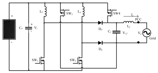
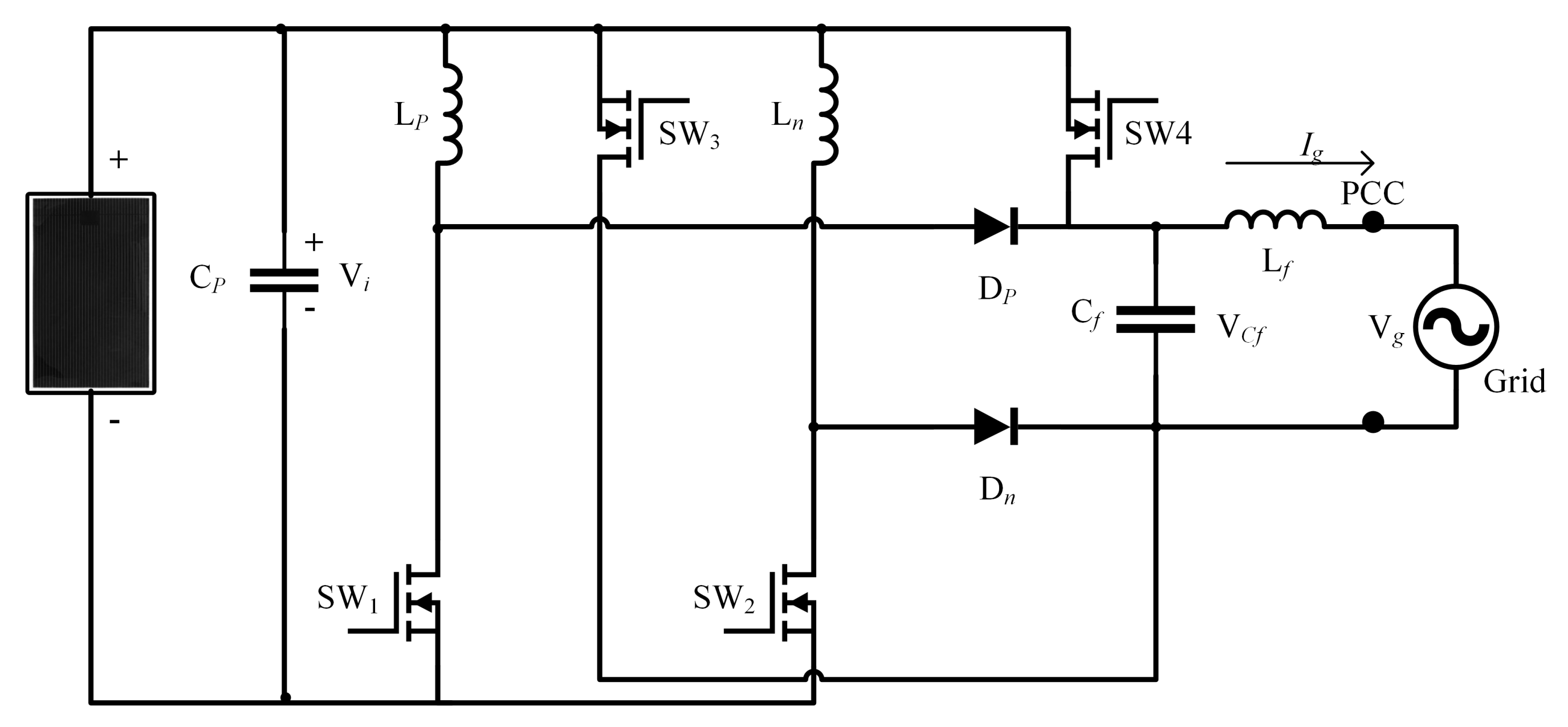
The BBSM topology is shown in Figure 1 it encompasses four semiconductor switches controlled devices, two uncontrolled devices (diodes), and a C-type filter. At the Point of Common Coupling, the proposed inverter intersects the grid (PCC). were employed for buck-boost operation and grid injection of PV energy. They also prevent inverter shoot-through issues. This increases system reliability while also making switching processes easier. During both half cycles of the reference, and are activated to energize the inductors and , respectively. The , as well as plays a crucial role in inductors’ discharge and energy injection into the grid. The load is assumed as pure resistive load .
Figure 1.
Buck-Boost Single-stage Microinverter.
The and switches have a high operating frequency. The and switches operates at low frequency. All of the switches have a built-in safety diode. The inverter can be operated in six distinct modes, three of these modes occurred during each half cycle of the common reference or control signal. These occurred in a row, i.e., one after the other. In both reference cycles, the BBSM topology operates similarly to a typical DC-DC buck-boost converter, except that the suggested inverter topology modulates on a quasi-sinusoidal duty-cycle.
The control strategy is essentially accomplished through a two-steps scheme: the first is achieved via the control of the PV array’s voltage by the inductors’ current imposition, the second is achieved via the control of the grid current via the output capacitor’s voltage imposition. The principle of operations is described with the aid of the control variables are as follows:
- Parameter O indicates the status of the output voltage half-cycle, during the positive part of the reference, O == 1, and switches and are in the ON state. During the negative part of the reference O == 0, and and are in the ON state. The reference cycle is obtained when is compared to 0.
- Parameter U indicated when the output voltage has to be increased U == 1, this is achieved through triggering switches or or to be stepped-down (decreased) then U == 0 and achieved when triggering switches or this is accomplished by comparing and .
- Parameter and indicates the charging / discharging process of and , respectively, as follows: = 1 & = 1, turn on / = 0 & = 1, turn on )/ this is generated by comparing the and inductor current .
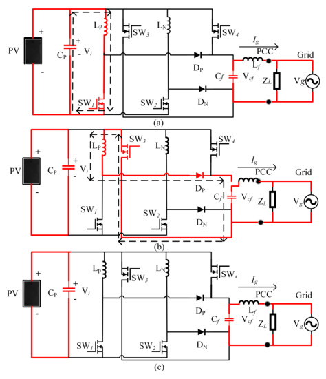
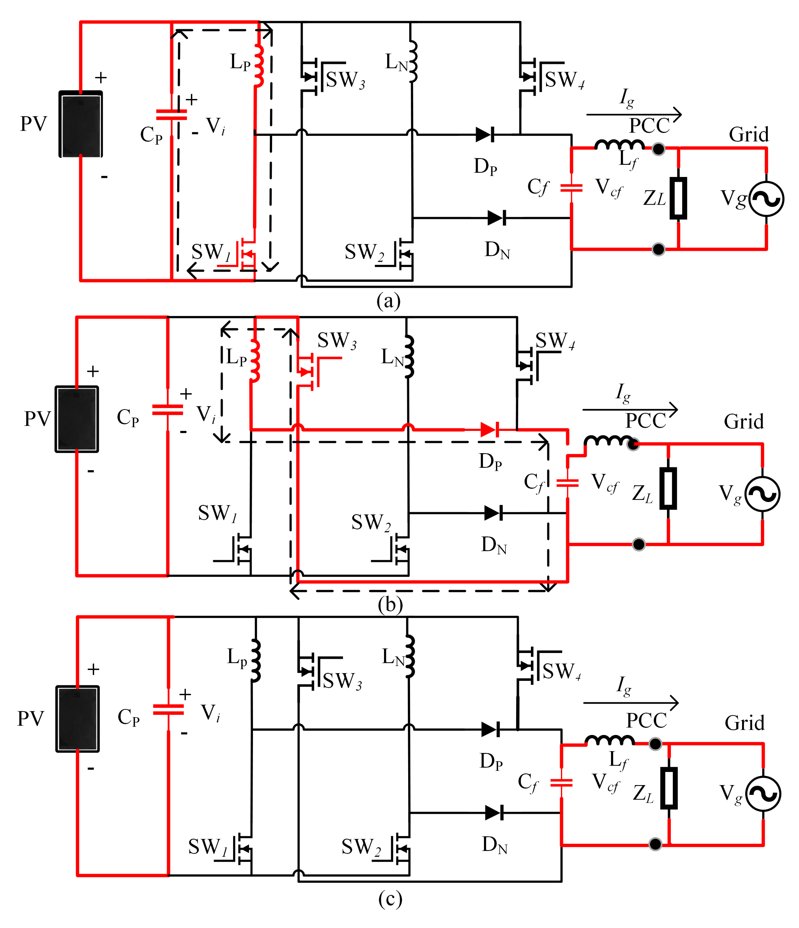
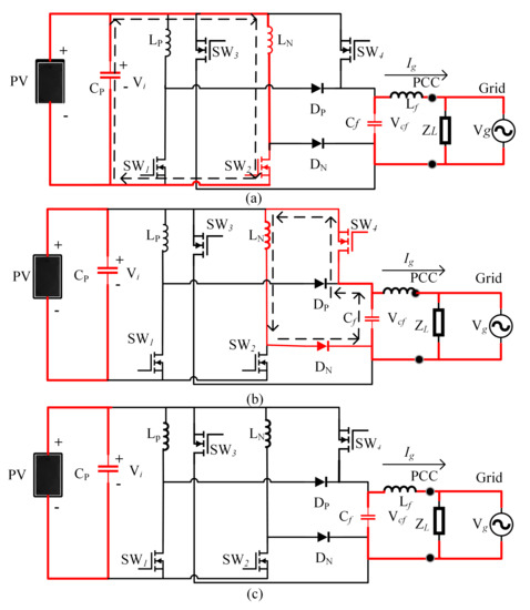
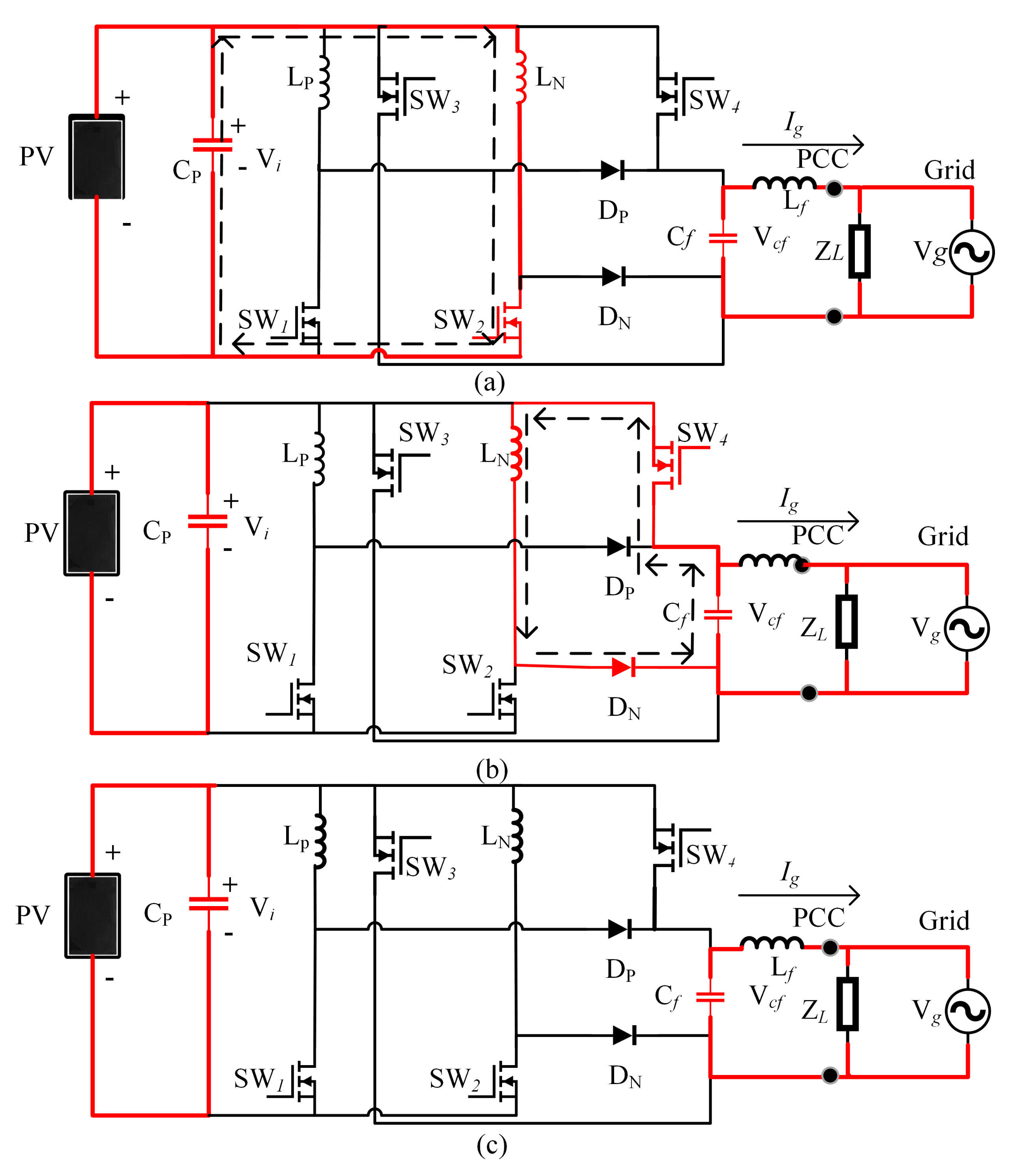
Table 2 summarises the state of passive and active components in each mode of operation. Figure 2 and Figure 3 depicts the three modes of functioning of the topology in the positive and negative half-cycles, respectively. In different modes, the highlighted components are active. It’s vital to remember that during each operation, only one switch is in the conduction path, even if another switch is on. This may help to lower the total power loss of the system.
Table 2.
Components operational status at each mode.
Figure 2.
(a) Circuits that are equivalent to Mode . (b) Circuits that are equivalent to Mode . (c) Circuits that are equivalent to Mode .
Figure 3.
(a) Circuits that are equivalent to Mode . (b) Circuits that are equivalent to Mode . (c) Circuits that are equivalent to Mode .
The operating mode is carried out for the current assessment of the inductor as shown in Figure 2a, and switch is activated due to this reason. Differential equations for control variables are derived from Figure 2a. Here is the input voltage and is the grid voltage, is the output filter capacitor, and is the load.
After storing the energy in during mode to provide the required voltage gain, the working mode is initiated. The stored energy is transferred through the output filter capacitor–load combination, while the positive half cycle diode becomes forward biased in addition to creating a closed-loop via as well as the inductor , meanwhile, is turned into its off status. The operating operation can be expressed using the differential equations from Figure 2b as follows;
When the energy stored in inductor () is transmitted to capacitor load combination (), the mode is then initiated. As shown in Figure 2c, the output energy of the filter capacitor is delivered under this mode.
The operation mode is employed to apply current to inductor , as shown in Figure 3a, and switch is enabled for this reason. The following differential equations for control variables are derived from Figure 3a.
After storing sufficient energy in the negative half cycle inductor () to provide the required voltage gain, the working mode is activated. The stored energy is delivered to the filter capacitor-load combination, while the diode becomes forward biased in addition, establishes a path of conduction via as well as the inductor , is triggered off mean. From Figure 3b, the following differential equations are found.
mode is activated, when all of the energy from the inductor () is shifted to the capacitor (). As shown in Figure 3c, the filter capacitor energy can be delivered to the output load in this mode.
To evaluate the proposed topology, the following assumptions are made.
- Equation (11) shows the relationship between (Grid frequency) and (Switching frequency of switches and ).
- The semiconductor devices device possesses ideal characteristics.
- Throughout each switching time-period , the grid voltage is considered constant.
- MOSFETs and diodes have zero forward resistance and infinite reverse resistance.
- The duty cycle remains constant during each switching period.
- The inverter’s operation is maintained DCM.
- The load is resistive
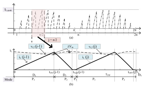
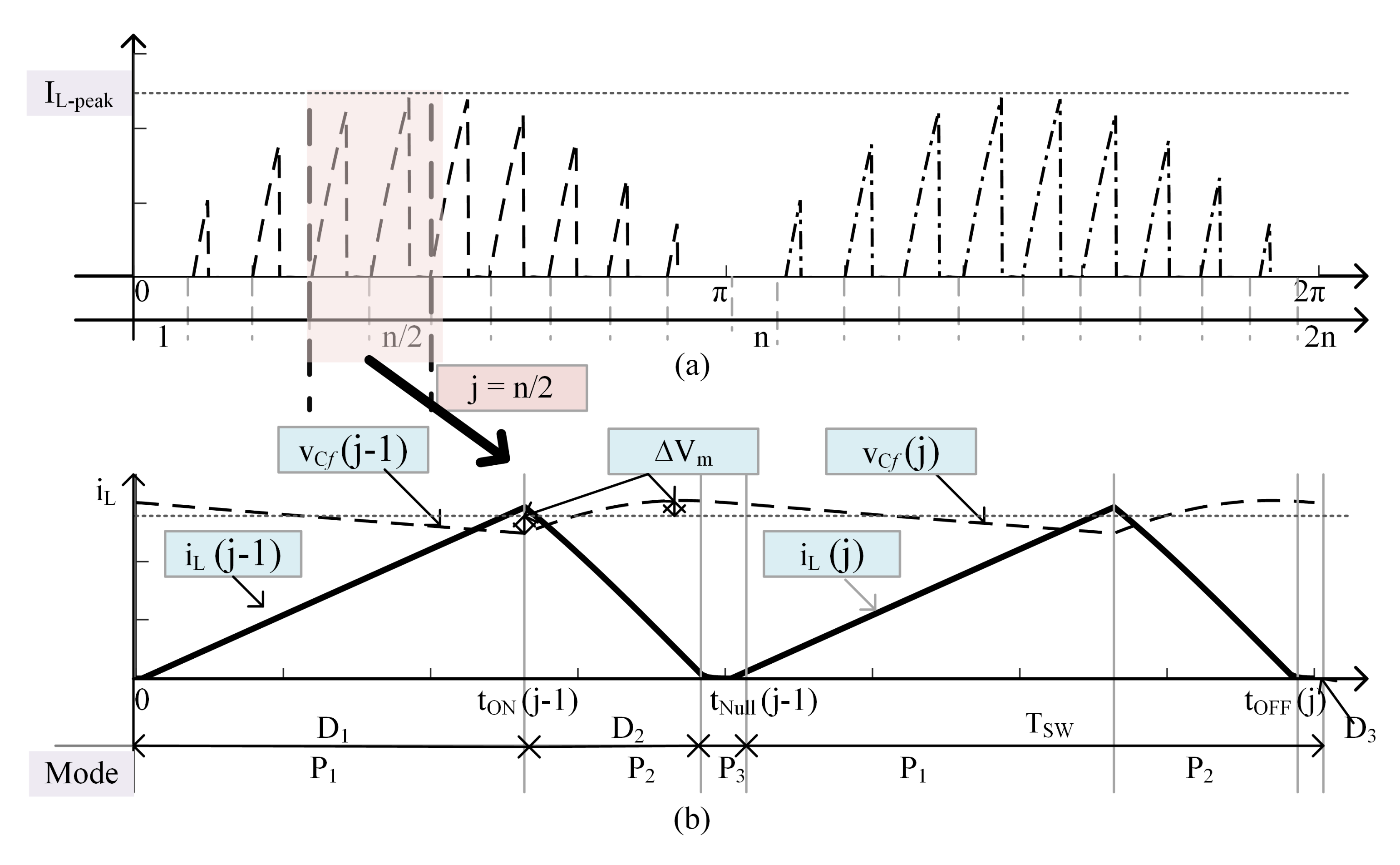
The and behave similarly during both reference cycles, they are referred to as L in the analytical section. Inductor current at the peak interval in zoomed in Figure 4b. In mode, the inductor current increases. For the jth switching period, the inductor charging current achieves its maximum value at . As the quantity of energy transferred to the output is determined by the magnetizing current of the inductor, the peak value of the current () is provided in (12) and depends on the output power. (13) can be used to express the energy stored in the inductor ().
Figure 4.
(a) Inductor current (), (b) Inductor current and capacitor voltage during the peak switching interval.
Using Equation (13), the average value of current in inductor throughout a swapping period expressed in Equation (14). As noted in (15), the current at output A is a sinusoidal changing current and that can be expressed as , as illustrated in the expression (14). As a result, the energy required on the output side can be written as (16). The peak output voltage is in this case. By equating the Formulas (13) and (16), the charging duty ratio may be stated as (17).
2.1. DCM Operational Requirement
The inductor current discharge completely in time , if the average value of the current is lesser than the maximum ripple. Until the next switching cycle, the current will stay zero. When this pattern occurs, the inverter is in DCM mode. If the suggested inverter topology meets DCM condition for the time duration , it operates in DCM mode throughout the grid cycle. The essential requirement for sampling duration of the grid voltage is applied as described in (22) for calculating the peak modulation index M limit for maintaining DCM functioning. In accordance with the conditions, the peak modulation index limit is calculated based on (23).
The peak output voltage, , is used here.
2.2. Elements for Energy Storage Design
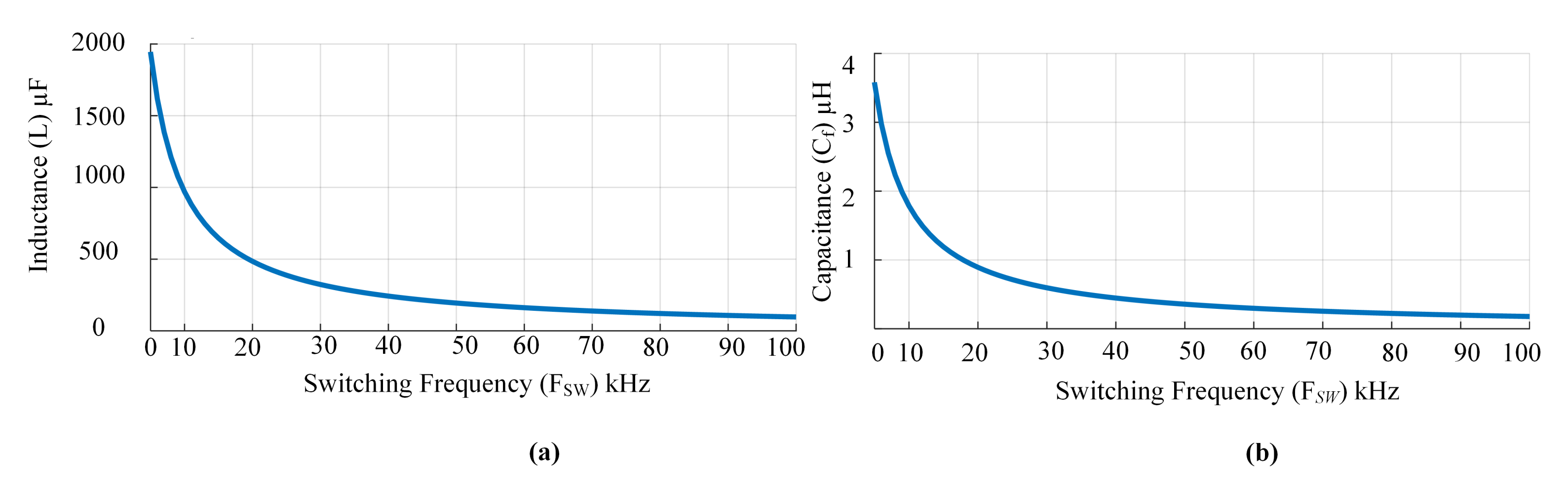
As the physical size of the inverter is determined by the size of its energy storage devices, the design of these elements is critical. Figure 4 depicts the inductor current . Energy is delivered in a discrete form since the inverter works in DCM. During each switching interval () Inductor L will store and transmits energy. Thus, a capacitor is used in the inverter topology. The inductor’s energy has been completely transferred to the capacitor Cf. During the peak phase (), it transfers most of the energy from L to . The inductor should be able to handle (), where is the maximum input power. This situation assures when the grid receives () during each grid cycle, hence (24) is derived from (13). Equation (25) may be used to calculate the inductor value by replacing (12) into (24). The relationship between L and is seen in Figure 5a from (25). The maximum power output of a Photo-Voltaic module determines the design value of L. This condition ensures that DCM will work at any power level.
Figure 5.
(a)The relationship between the switching frequency () and the inductance value. (b) The relationship between the switching frequency () and the capacitance value.
2.3. Power Device Selection
The whole cost and performance of a system are affected by the rating of the power devices in an inverter, which includes storage duration, current gain, and switching frequency. the calculation of voltage, as well as current load on power equipment, can be calculated. Switches maximum voltage is the same as the capacitor’s maximum voltage. Similarly, the peak current of the switches matches the maximum inductor current. The total active switch stress SS must be computed if the inverter has k switching devices as stated in (28) using the RMS current and the voltage . Table 3 lists all of the switches RMS current as well as the peak voltage expressions.
Table 3.
Current and voltage expressions.
3. BBSM Topology Design
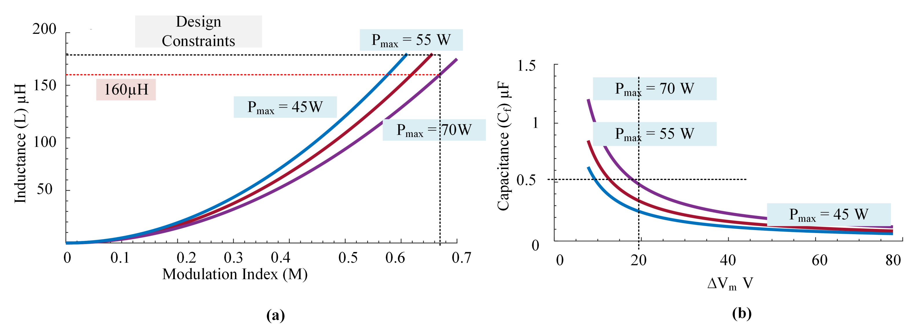
The passive elements design relation was derived from the analysis of the BBSM topology, while designing, the nominal power of the inverter is considered equal to the maximum power of the PV module. Thin-film PV modules are widely employed in BIPV applications, according to [16]. For the purpose of inverter validation, we have looked at the first solar PV module. = 110 V, = 70 W, = 50 Hz, = 73 V. On the basis of Figure 5, the optimal switching frequency of 50 kHz was chosen, resulting in 2n = 1000. For these specifications, the maximum modulation index is derived using (23) as . The peak permissible inductance for the discontinuous mode of operation (DCM) is estimated using (25) as . Black dotted line in Figure 6a shows the two constraints and for the determination of the inductance value. It can be shown that these two constraints are satisfied when the inductance value is . The filter capacitor value for output voltage is plotted in Figure 6b based on (27). The capacitance value is between for a peak ripple of . Thus, in this project capacitor is chosen. The DC-link capacitor is determined as for this project [13].
Figure 6.
(a) Inductance value vs. modulation index. (b) versus capacitance value for various power ratings.
4. Loss Analysis
Using the elements design value the expected losses of the BBSM topology is discussed in this section. The power loss analysis includes core loss, conduction loss and switching loss evaluation.
4.1. Core Loss
Changing magnetic flux fields causes core loss within a material. The core loss density () is a function of , and , where () is half of the flux swing as shown in (29). In order to approximate the constants core loss charts are utilised.
Number of turns (N). The ripple current in the inductor is △, and the air gap in the magnetic core is . The permeability of the air gap is , which is 4 × . As a result, the equation for is (32)
The magnetic core’s mean path length is , and the cross-sectional area is .
4.2. Conduction Loss
The total conduction loss is equal to the summation of the inductor loss and conduction loss in power devices.
The inductor conduction loss can be calculated using the average inductor current as well as the inductor’s series resistance from the (33).
In the BBSM, the switch , as well as switch , operates in a symmetrical way for both half cycles, resulting in the same conduction losses, as determined by (34).
The conductive loss of a diode is estimated as (36) using the power loss accompanied with the fixed voltage drop () as well as the resistance .
Here, the is given in Table 3, and are determined from the datasheet of the diode.
4.3. Switching Loss
The switching loss of and switches is negligible since they operate at a low switching frequency. Similarly, because the inverter works in DCM, the diode’s switching loss owing to reverse recovery is zero. Due to the DCM operation, turn on losses are nil in switches and . As a result, the inverter’s total switching losses are indicated in (36).
The switch’s Turn OFF energy loss as well as fall time may be found in the datasheet. The inverter’s losses are estimated using the parameters reported in Table 4. The BBSM inverter’s power loss is documented in Table 5. All topologies losses are computed using a 70 W system.
Table 4.
Power loss calculating parameters.
Table 5.
The Power loss of the BBSM inverter.
5. Design Validation
In order to validate the proposed BBSM topology a simulation and experimental test has been conducted as given below.
5.1. Simulation Results
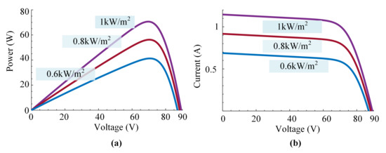
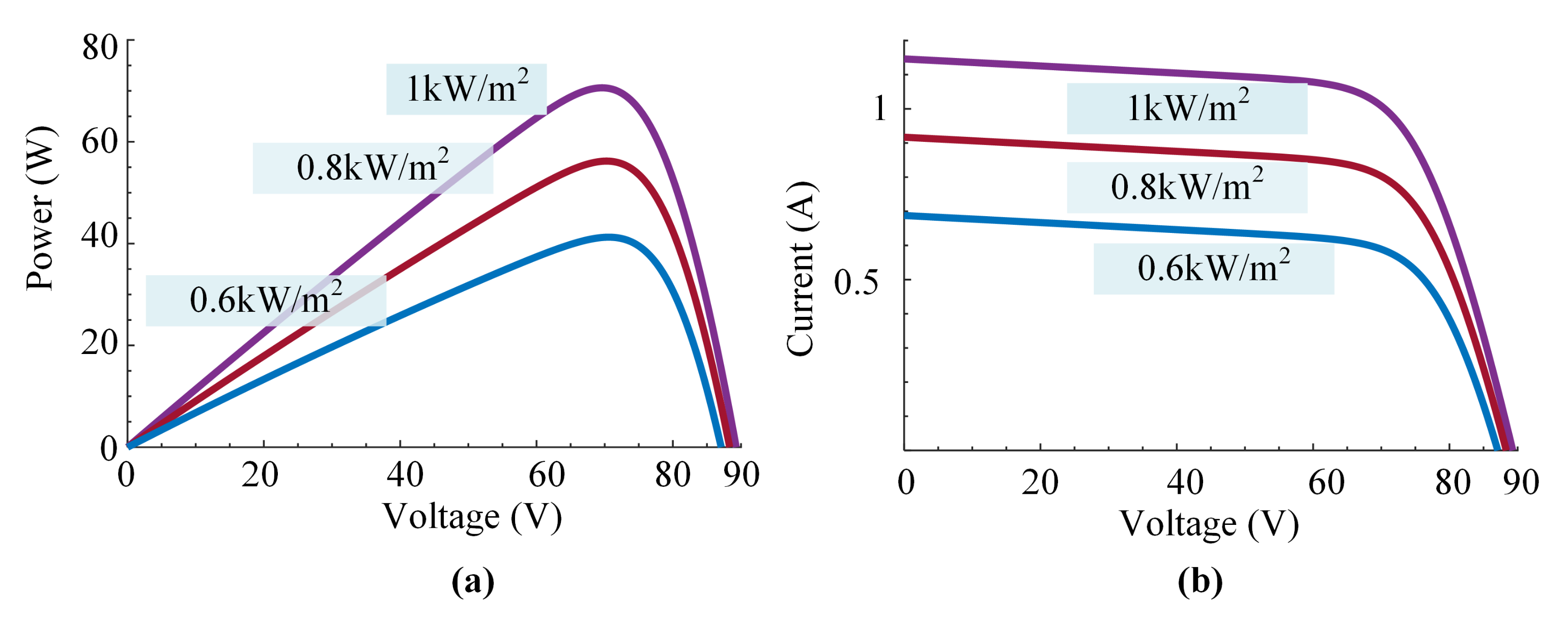
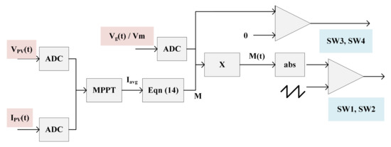
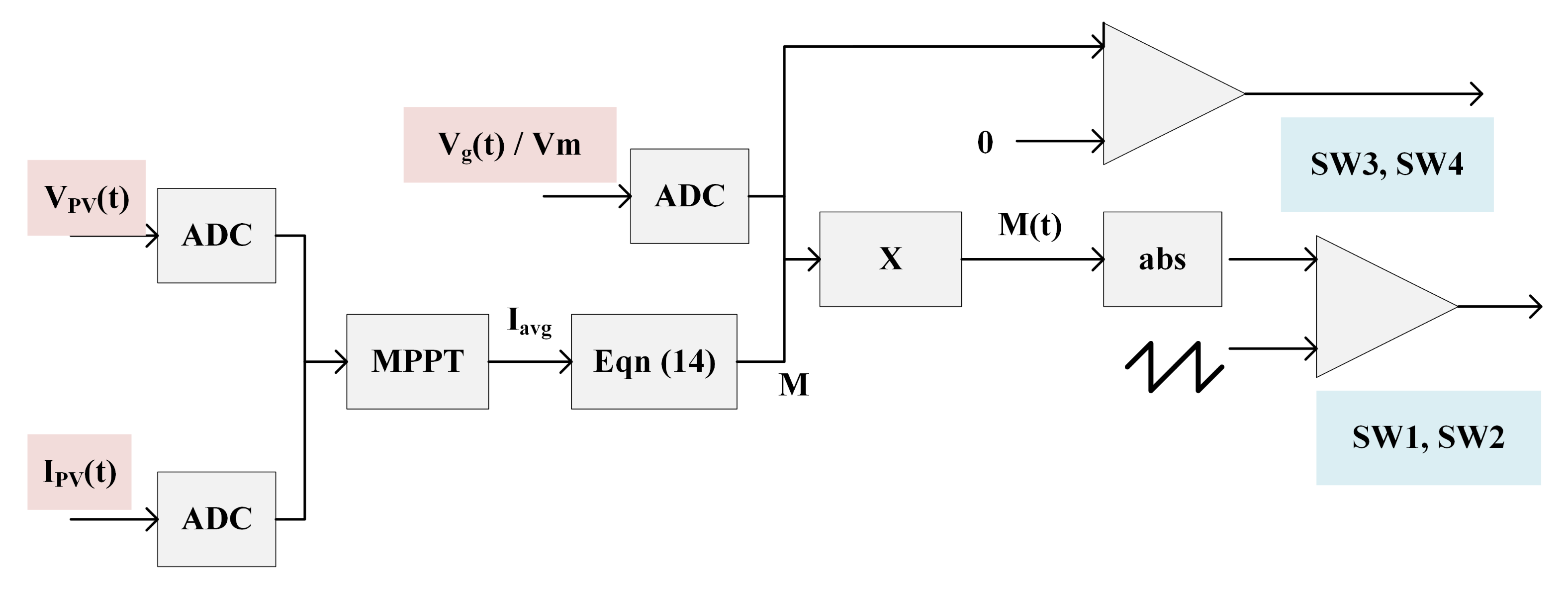
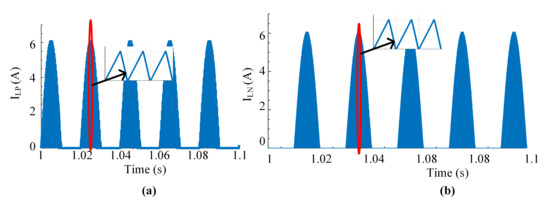
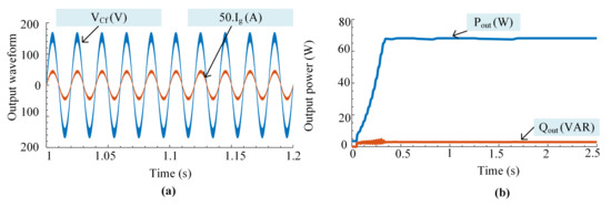
The simulation using MATLAB / Simulink is carried out for the proposed microinverter and the ratings, as well as component values are displayed in Table 6. A thin film Photovoltaics module FS 270 which is of 70 W is considered, with the approaches given in [17,18] are being used to simulate it for simulation. Figure 7a,b show the I-V and P-V graphs generated from the model for 1 kW/m, 0.8 kW/m and 0.6 kW/m, respectively. The testing control circuit and the block diagram of the inverter is given in (20) and plotted in Figure 8, respectively. In this project, the Perturbation and Observation () approach suggested in [19] is employed for MPPT by sampling and . At a maximum power of 70 W, Figure 9a,b show the current flow through the inductors and , respectively. The theoretical calculations of the peak current through the inductor and for the DCM functioning of the BBSM inverter topology is convincingly validated. At the maximum power rating, the inverter’s output voltage and current are 110 V and 0.636 A, respectively, as shown in Figure 10a. The active power P and reactive power Q in the grid are plotted in Figure 10b.
Table 6.
Element values obtained from the design [5].
Figure 7.
(a) PV voltage index versus Power. (b) PV voltage versus current for different irradiation level.
Figure 8.
Block diagram of the control technique used for BBSM.
Figure 9.
(a) Current through inductor . (b) Current through inductor .
Figure 10.
(a) Injected current and output voltage. (b) Active and reactive power at the output side.
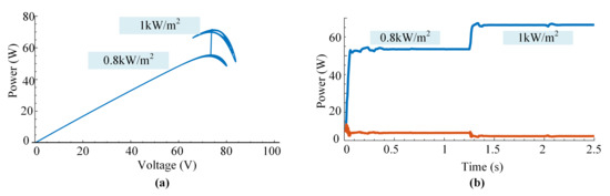
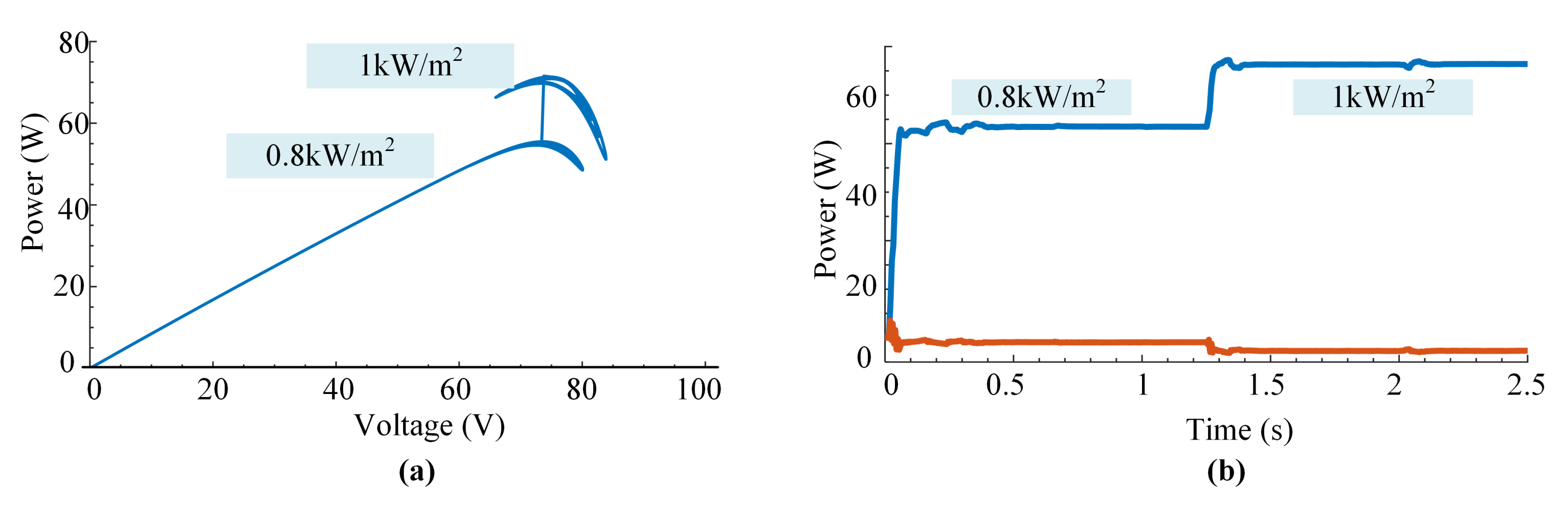
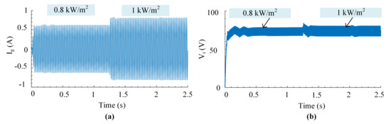
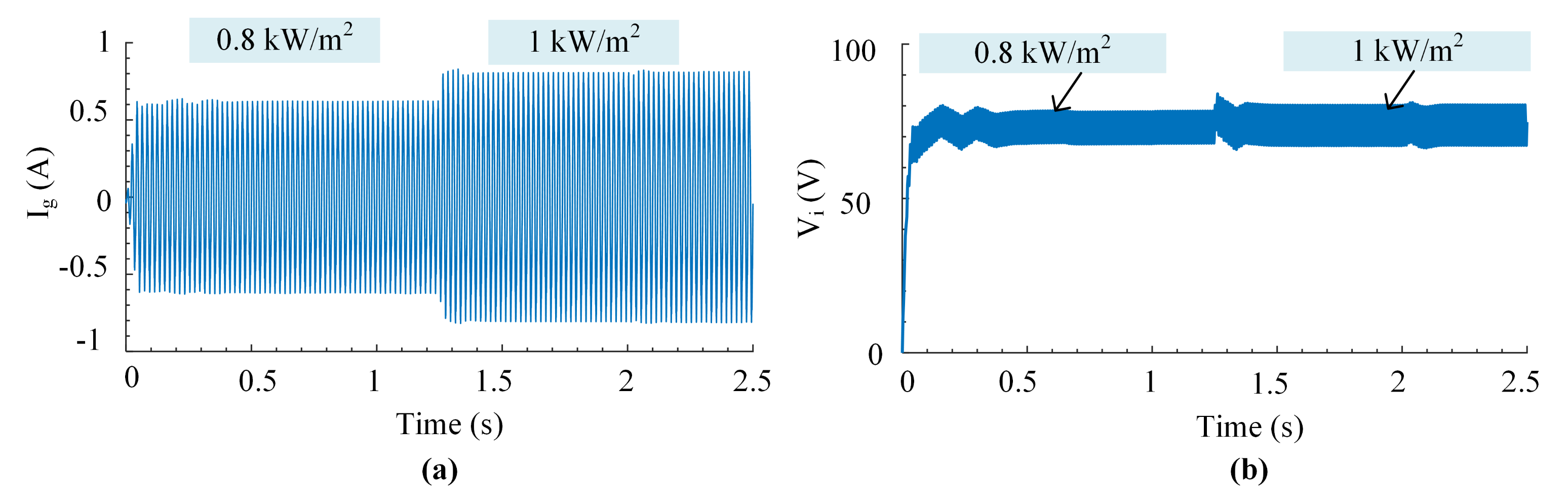
Further research of the suggested inverter’s open-loop control was conducted by changing the degree of irradiation level. The MPPT operation is shown in Figure 11a while adjusting the level of irradiation ( to ) in 1.25 s. Despite the fact that it functions in the MPP field, further research in this area is essential for exact operation. During irradiation change, Figure 11b and Figure 12a,b show alterations in output current, output power, and input voltage, respectively. The results show that the inverter is operating correctly when the irradiation changes.
Figure 11.
(a) curve of MPPT. (b) Changes in active and reactive power under irradiation.
Figure 12.
(a) Variation in the output current . (b) Variation in input voltage with respect to changes in irradiation levels.
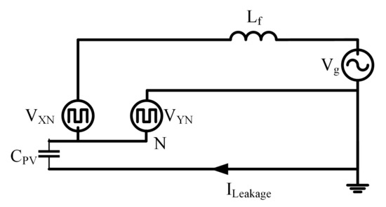
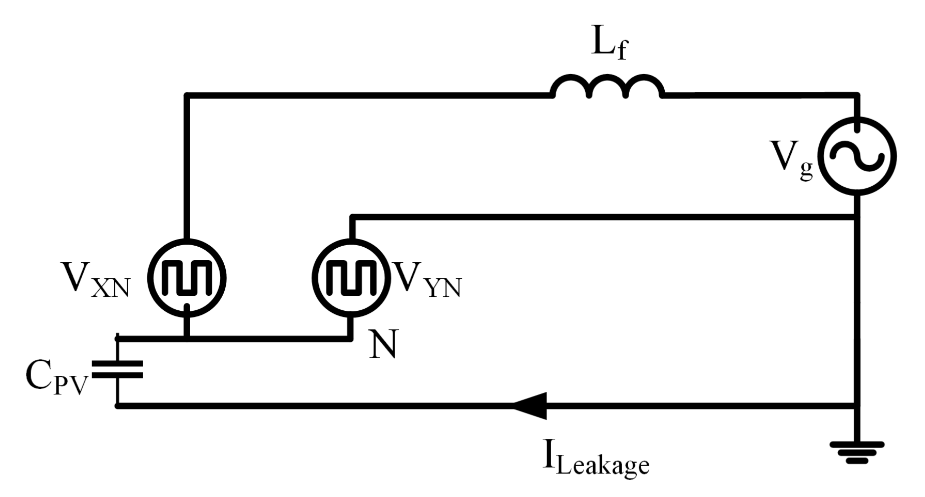
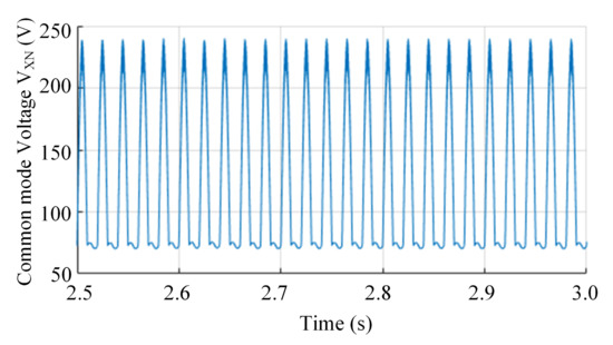
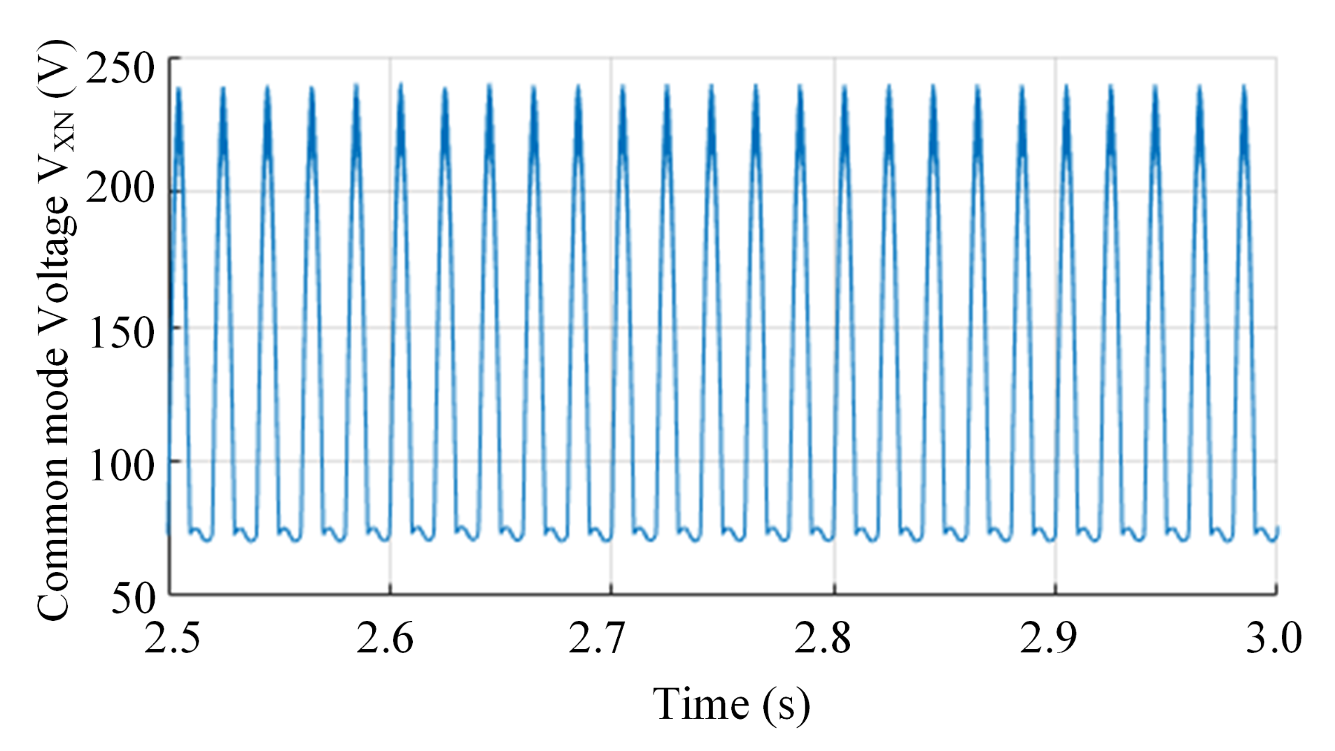
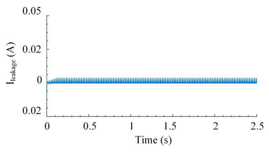
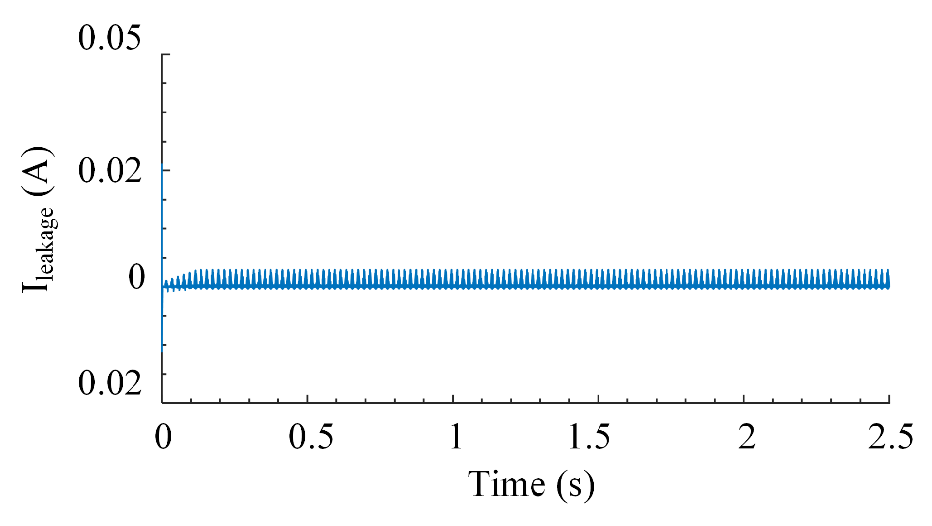
To evaluate the flow of leakage current in the proposed inverter, a parasitic capacitance of 70 nF was used in the simulation [20]. According to German regulations DIN VDE 0126-1-1, if the leakage current exceeds 300 mA (RMS), the inverter must be removed from the grid. As shown in Figure 13, a circuit for resonance condition is created for the transformerless inverter. PV parasitic capacitance () as well as filter inductor () are included in the resonant circuit. X, and Y are the inverter’s terminals, which are coupled to the single-phase grid via . As shown in Figure 13, the inverter maybe simplified into an equivalent circuit consisting of and . As a result, leakage current is determined by as well as . (37) can be used to define the Common Mode Voltage (CMV). The leakage current travels via the parasite capacitance and to the grid when there is a differential. As demonstrated in Figure 14, the proposed topology has low-frequency components and . As the voltage differential between the BIPV module’s ground and the grid is low-frequency, the parasitic capacitance’s equivalent impedance is high. This high impedance, as seen in Figure 15, restricts the flow of leakage current . In this simulation, a parasitic capacitance of 70 nF was employed to check the [20]. The proposed inverter’s leakage current is negligibly tiny, as shown in Figure 15.
Figure 13.
BBSM equivalent circuit to show path for leakage current.
Figure 14.
Common mode voltage .
Figure 15.
Leakage current at = 70 W.
5.2. Experimental Results
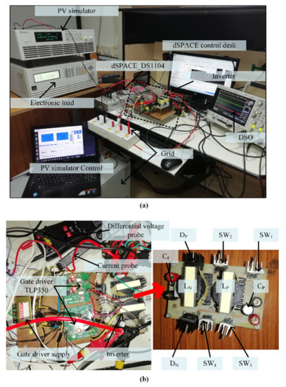
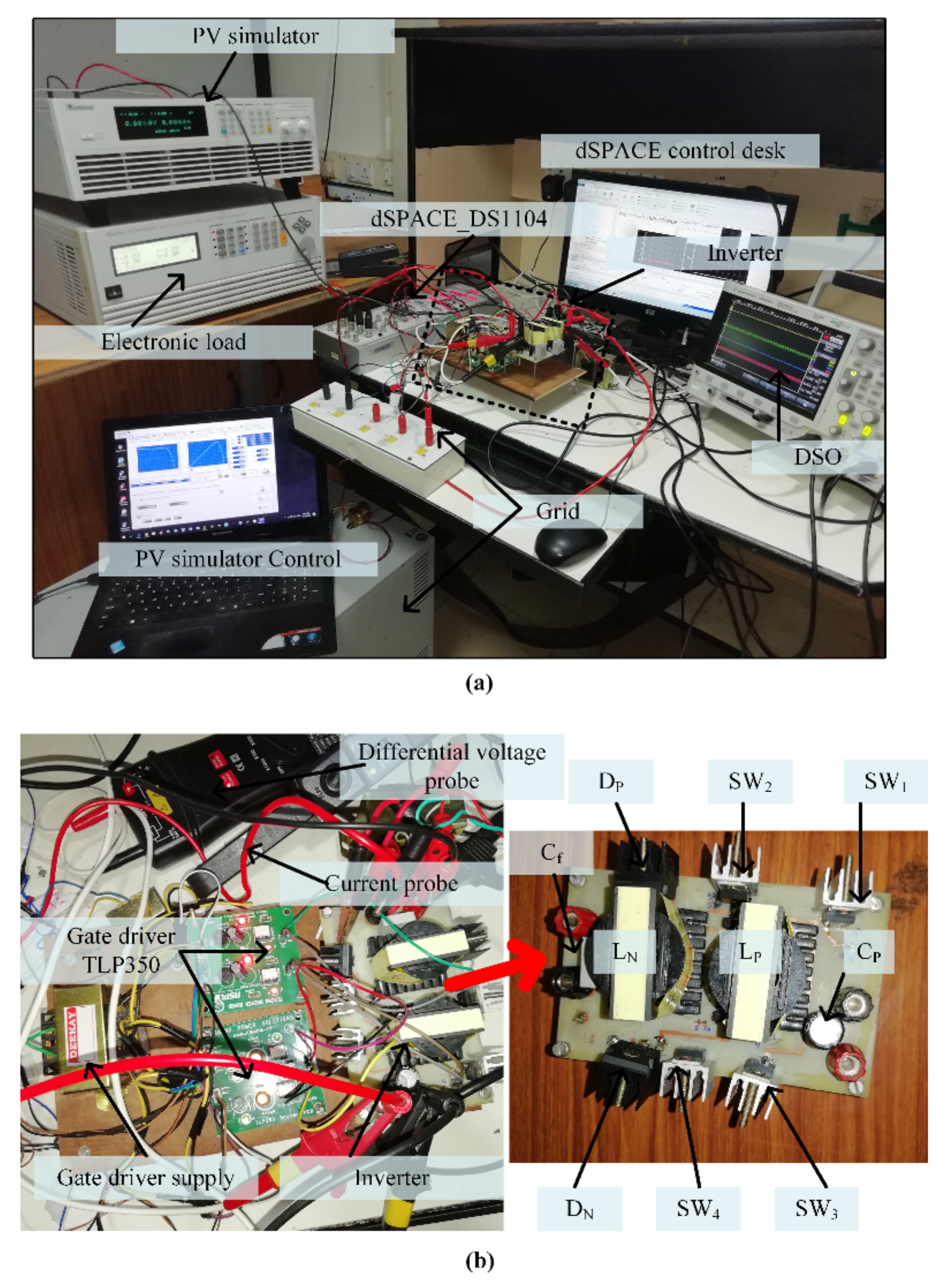
Based on the specifications in Table 6, an experimental model of a 70 W, 110 V, 50 Hz inverter was designed. In Figure 16a, the experimental settings in the laboratory are shown, and in Figure 16b, the proposed BBSM topology is shown. In the experimental research, the chroma programmable DC power supply 62150H-600S solar array simulator was utilized to simulate the identical simulated Photovoltaic module characteristics. For loading, the programmable AC/DC electronic load 63802 was employed. A chroma 3-phase programmable AC source 61704 was used to duplicate the grid. The switching strategy was created in MATLAB in addition it is linked to the dSPACE-1104 control desk in the control area. All waveforms were captured using a DSOX3014 oscilloscope.
Figure 16.
(a) Setup for the experiment. (b) Power circuit of BBSM.
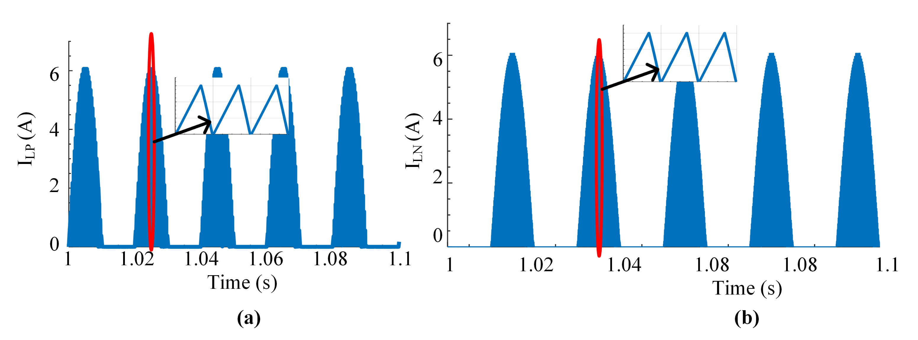
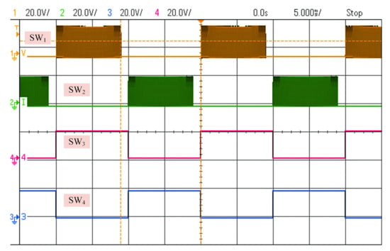
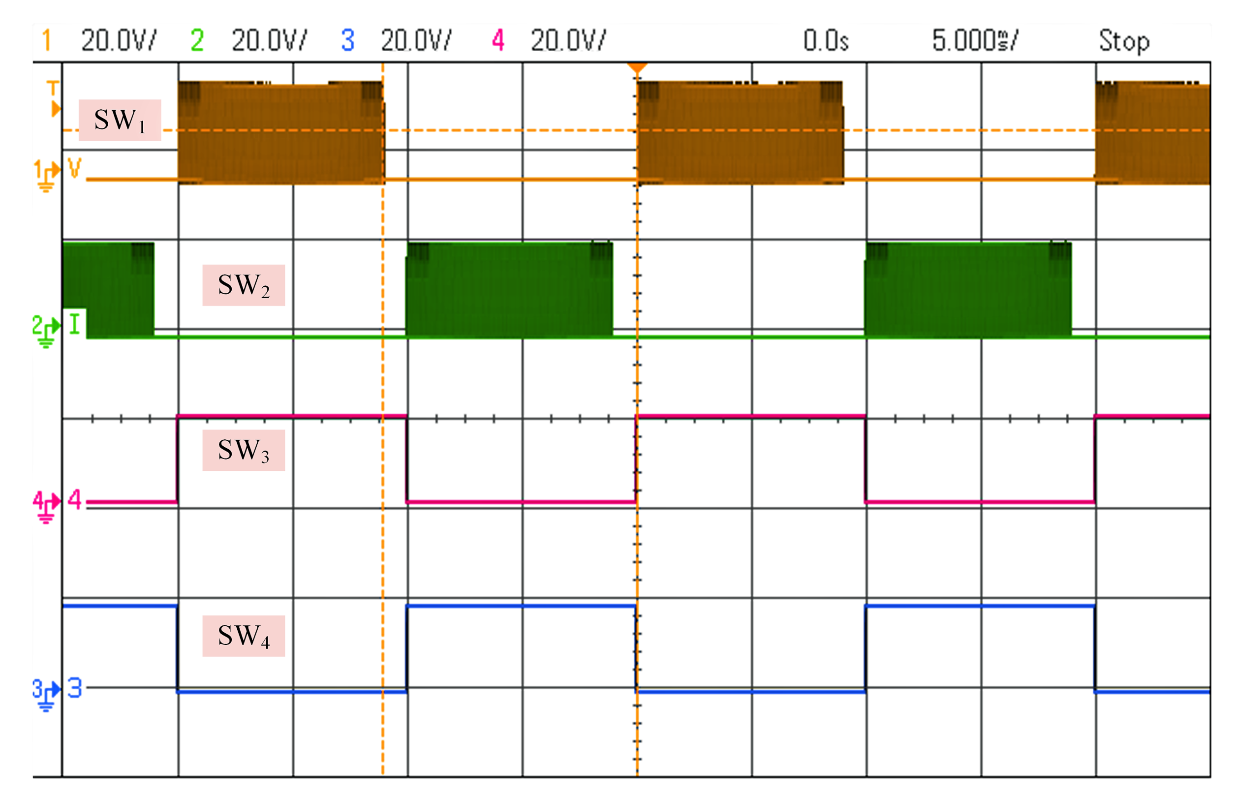
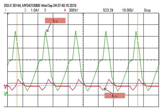
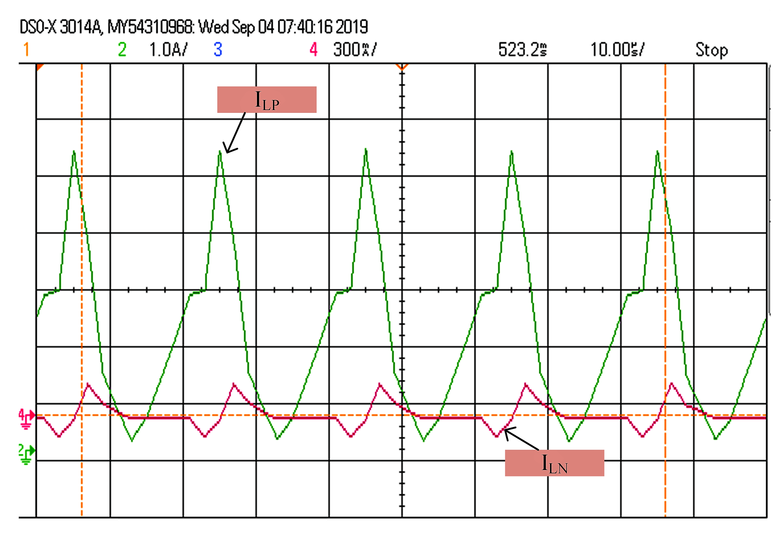
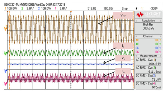
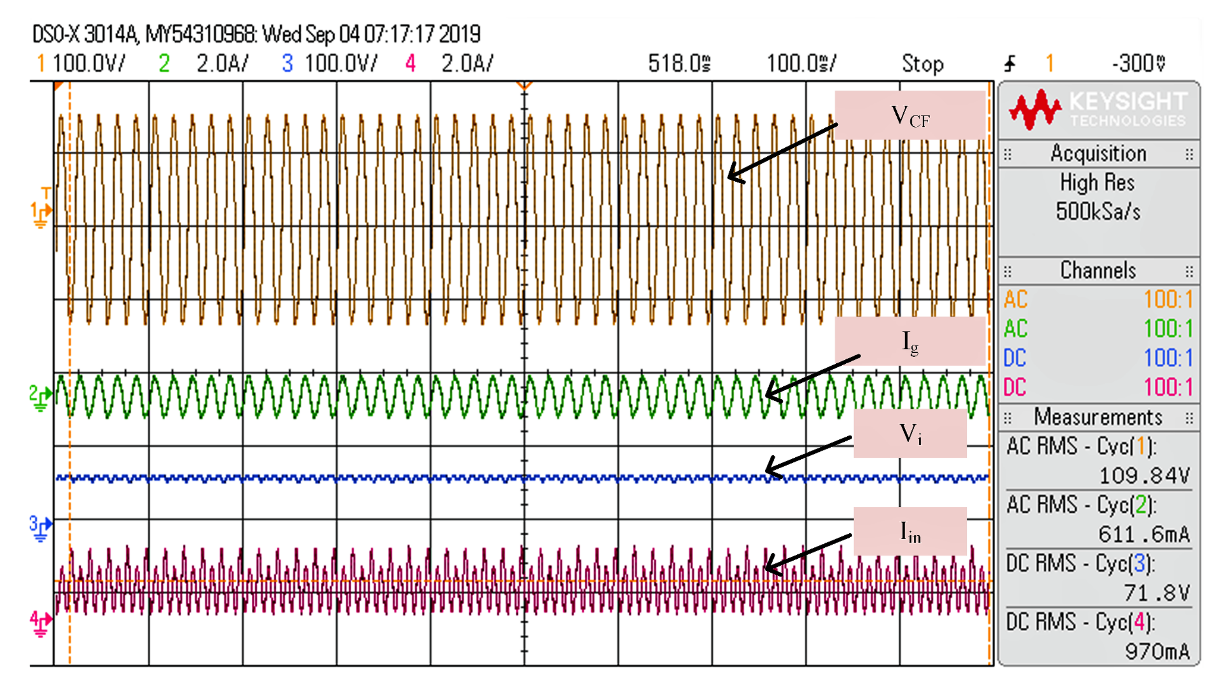
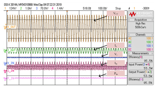
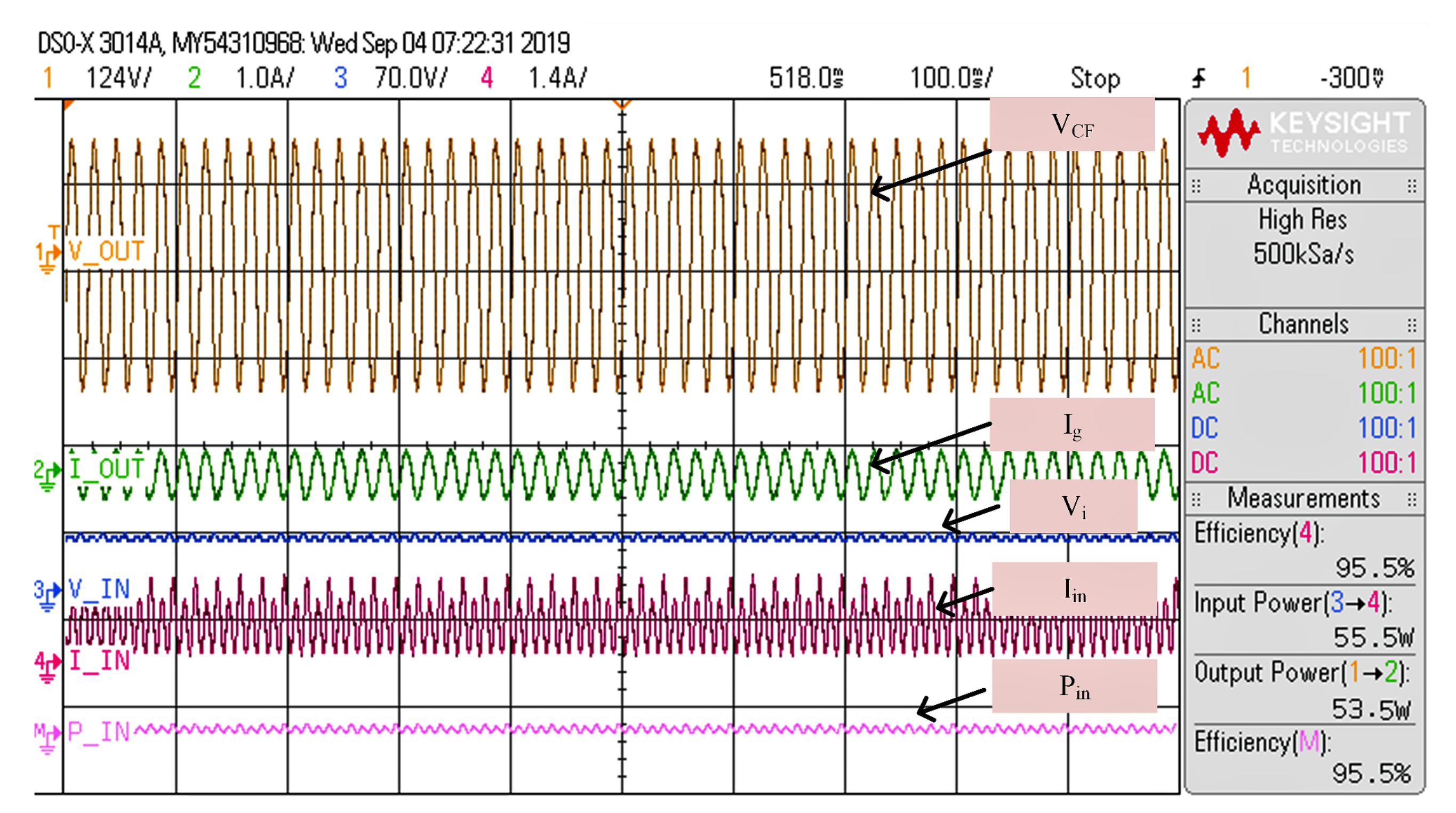
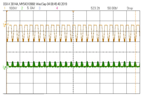
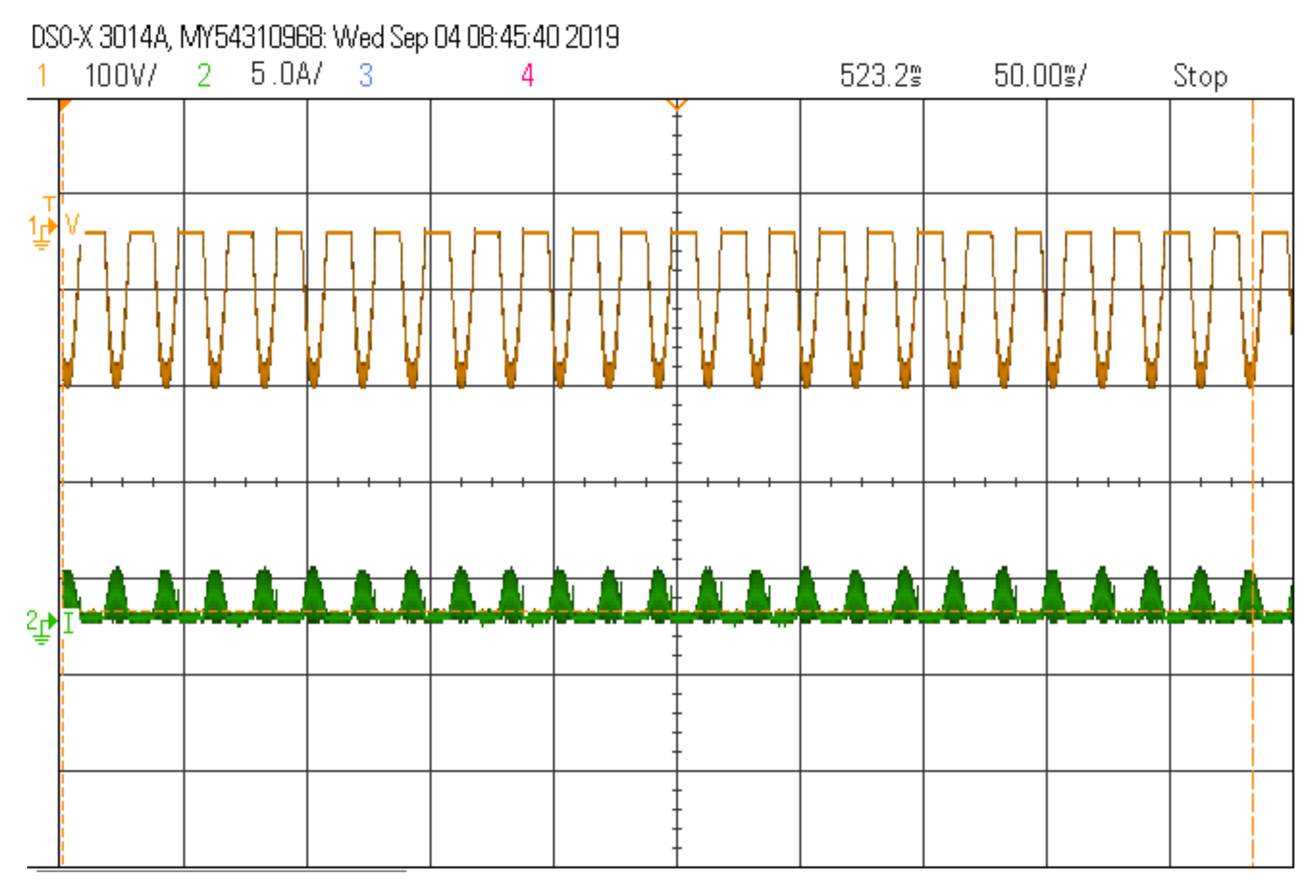
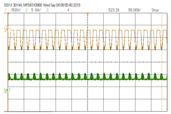
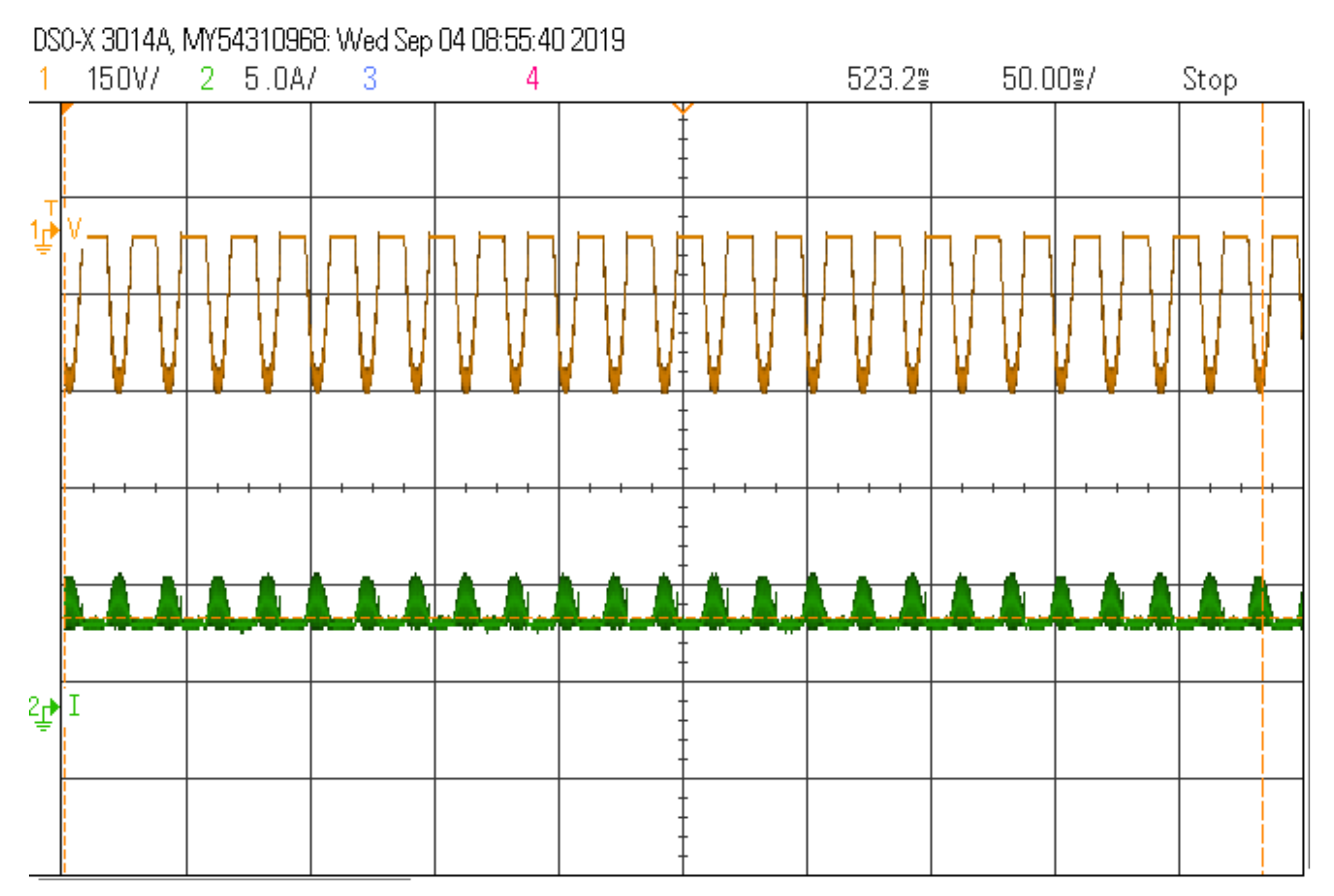
Figure 17 shows the switching pulses created by the dSPACE-1104 by using the TLP350 gate driver. As mentioned in the theory, as well as , represent 50 kHz pulses, while and represent pulses at 50 Hz. Currents through and with a magnified view during = 70 W are shown in Figure 18. It clearly validates the inverter’s DCM functioning and of around 6 A during = 70 W, as described in the theoretical analysis. Figure 19 shows the output voltage and current in relation to the input voltage and current at steady state. The output voltage and current RMS values are the same around the values analyzed and simulated. From Figure 19 the efficiency is obtained is 96.4% as given in (38). As expected from the theoretical analysis efficiency is above 95%.
Figure 17.
Switching pulses at = 70 W.
Figure 18.
Inductor currents and during = 70 W.
Figure 19.
Steady-state output and input voltage and current waveforms during = 70 W.
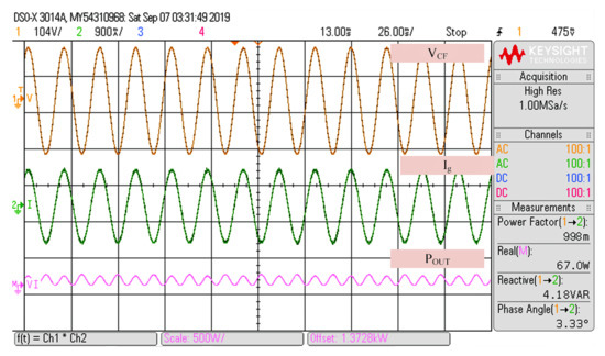
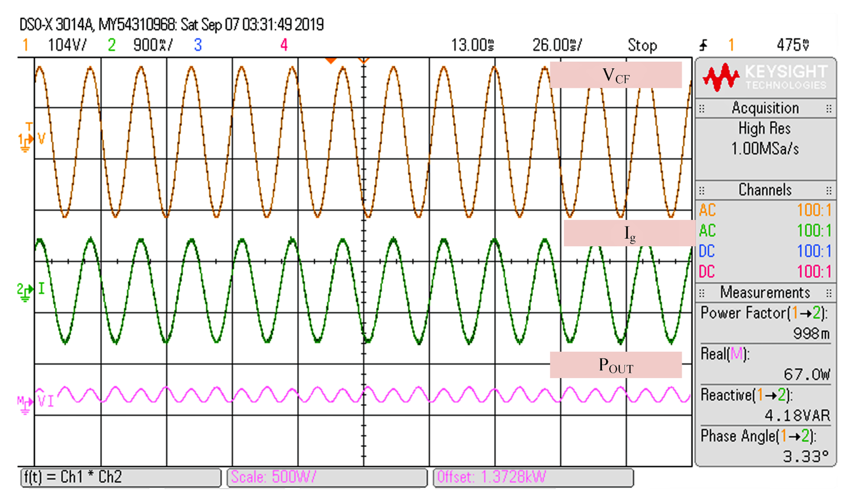
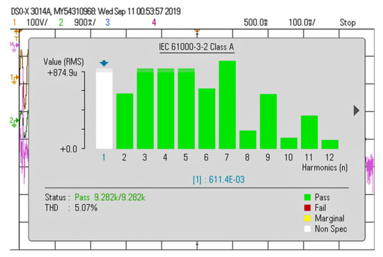
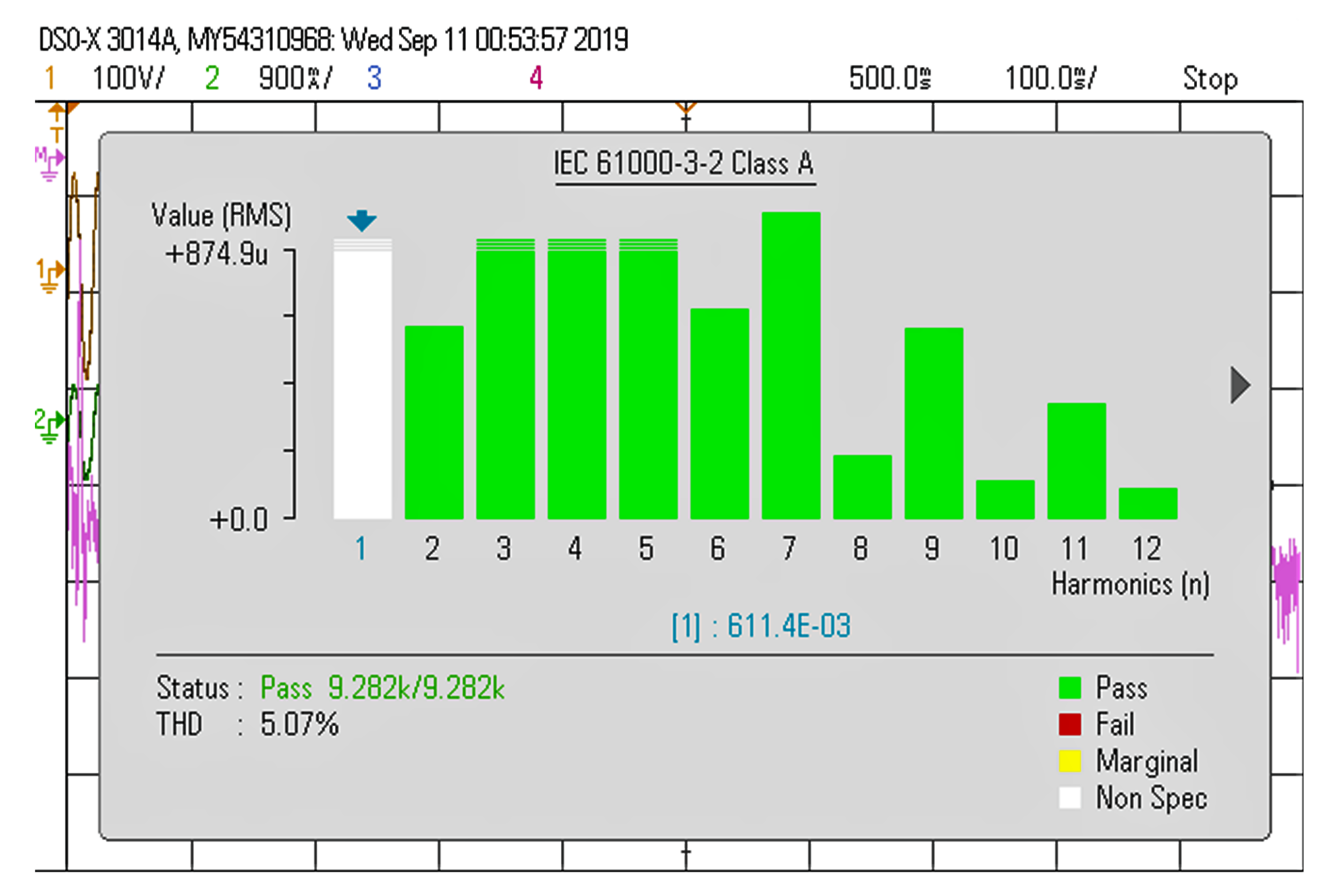
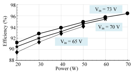
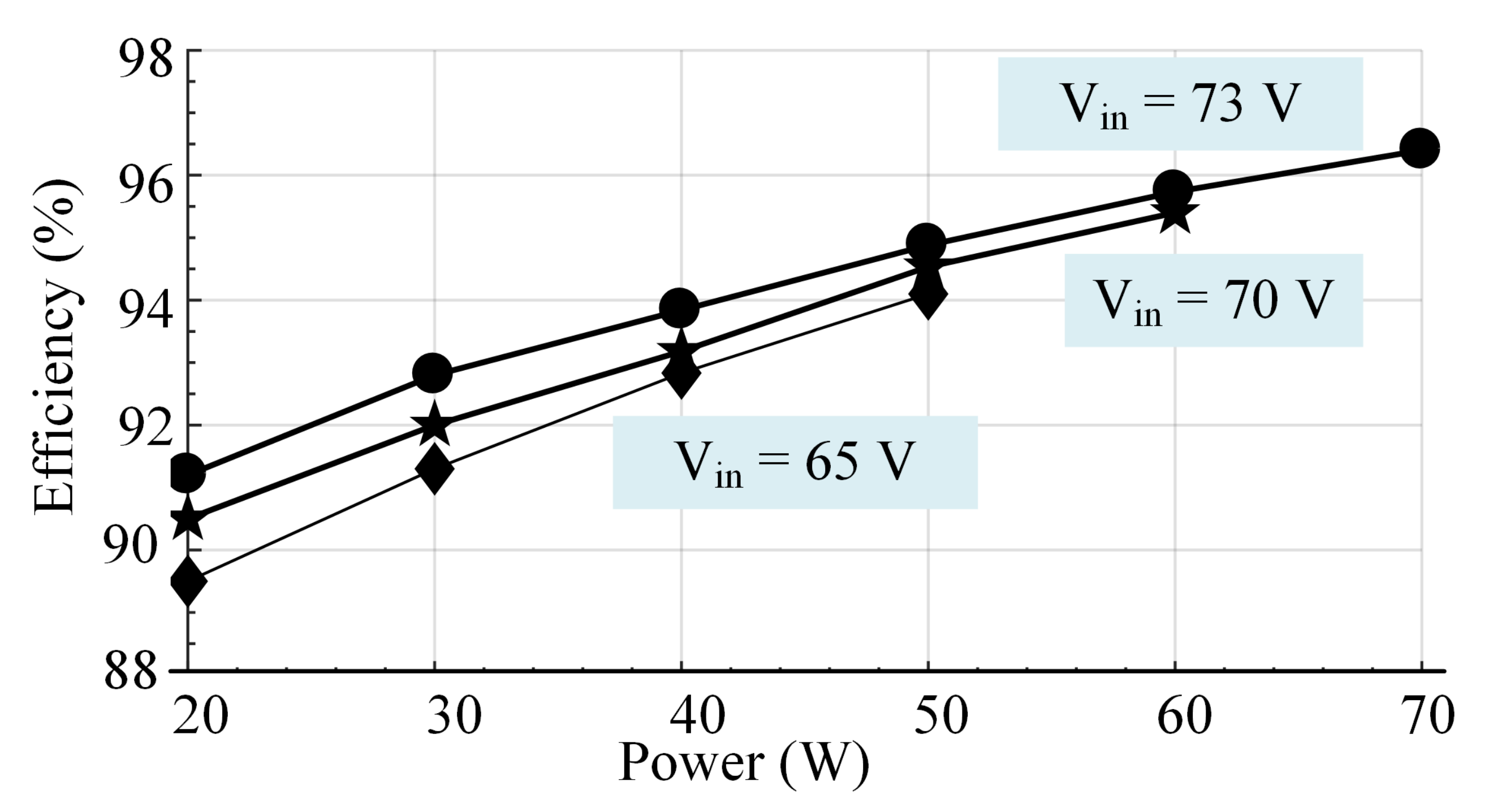
The waveforms of real power, phase angle, reactive power, current, voltage, power factor, and apparent power during = 70 W are shown in Figure 20. It is evident that the power factor is approximately 1. The injected current from the inverter’s Total Harmonic Distortion (THD) and Fast Fourier Transform (FFT) values are shown in Figure 21. The THD value of the current fed to the grid is around 5%. The input current, voltage, and steady-state output at 0.8 kW/m are shown in Figure 22, along with the efficiency calculation. Various input voltages inverter efficiency curve is shown in Figure 23. Voltage across and current through the MOSFETS and Diodes are shown in Figure 24 and Figure 25 respectively. The various values of efficiency from the proposed topology in low to nominal power operation is determined using a DC power supply in addition to a resistive load. Table 7 tabulates the comparison between simulation and experimental results, it clearly shows that due to the use of real time elements efficiency during experimental test is slightly lower.
Figure 20.
Power quality measurements during = 70 W.
Figure 21.
THD of injected current at = 70 W.
Figure 22.
Input and output voltage and current with efficiency at 800 W/m.
Figure 23.
Efficiency curve of the proposed inverter.
Figure 24.
Voltage across and current through the MOSFET.
Figure 25.
Voltage across and current through the Diode.
Table 7.
Comparison of results obtained using simulation and experimental study.
5.3. Comparison of Topologies
The BBSM uses fewer switches in the conduction path, according to a comparison of other microinverters in Table 8. Other topologies efficiency were determined using the same criteria used in this study. The BBSM topology is more efficient and has less passive elements than other topologies, making it excellent for BIPV applications. Furthermore, the proposed inverter has a negligible leakage current. When compared to other microinverters, BBSM is more efficient and reliable due to the employment of an appropriate number of components in the conduction channel.
Table 8.
Comparison of different topologies [5].
6. Conclusions
A buck-boost single-stage microinverter (BBSM) with fewer number of elements, with high efficiency and reliability were proposed in this paper. Due to the limited number of components, a higher performance is achieved. Design details of all the elements were derived in the paper. MATLAB/Simulink simulation and experimental setup was used to verify the design technique of the inverter systems. The results of the BBSM topology shows that it had negligently low leakage current with buck-boost performance, high operational efficiency, THD level for the injected current is within the limit, and prevented shoot-through. According to a comparison examination of the proposed inverter with similar topologies it shows that proposed topology can be recommended topology for Building Integrated PV system.
Author Contributions
Conceptualization, D.M.; methodology, D.M.; software, D.M.; validation, D.M. and R.C.N.; formal analysis, D.M., M.E.F. and R.K.M.; investigation, D.M., A.S. and P.S.; resources, D.M.; data curation, D.M. and R.C.N.; writing—original draft preparation, D.M., R.C.N. and M.E.F.; writing—review and editing, D.M., R.C.N. and M.E.F.; visualization, D.M. All authors have read and agreed to the published version of the manuscript.
Funding
This research received no external funding.
Institutional Review Board Statement
Not applicable.
Informed Consent Statement
Not applicable.
Data Availability Statement
Not applicable.
Conflicts of Interest
The authors declare no conflict of interest.
References
- Li, G.; Xuan, Q.; Akram, M.; Akhlaghi, Y.G.; Liu, H.; Shittu, S. Building integrated solar concentrating systems: A review. Appl. Energy 2020, 260, 114288. [Google Scholar] [CrossRef] [Scilit]
- Mousa, O.B.; Kara, S.; Taylor, R.A. Comparative energy and greenhouse gas assessment of industrial rooftop-integrated PV and solar thermal collectors. Appl. Energy 2019, 241, 113–123. [Google Scholar] [CrossRef] [Scilit]
- Bastidas-Rodriguez, J.D.; Franco, E.; Petrone, G.; Ramos-Paja, C.A.; Spagnuolo, G. Maximum power point tracking architectures for photovoltaic systems in mismatching conditions: A review. IET Power Electron. 2014, 7, 1396–1413. [Google Scholar] [CrossRef] [Scilit]
- Zare, M.H.; Mohamadian, M.; Beiranvand, R. Single-stage AC module with series power decoupling capability for connecting PV to a single-phase power grid. IET Power Electron. 2016, 10, 517–524. [Google Scholar] [CrossRef] [Scilit]
- Chander, A.H.; Kumar, L. MIC for reliable and efficient harvesting of solar energy. IET Power Electron. 2018, 12, 267–275. [Google Scholar] [CrossRef] [Scilit]
- Ahmad, A.A.; Abrishamifar, A.; Samadi, S. Low-frequency current ripple reduction in front-end boost converter with single-phase inverter load. IET Power Electron. 2012, 5, 1676–1683. [Google Scholar] [CrossRef] [Scilit]
- Hu, Y.; Du, Y.; Xiao, W.; Finney, S.; Cao, W. DC-link voltage control strategy for reducing capacitance and total harmonic distortion in single-phase grid-connected photovoltaic inverters. IET Power Electron. 2015, 8, 1386–1393. [Google Scholar] [CrossRef] [Scilit]
- Mathew, D.; Naidu, R.C. Investigation of single-stage transformerless buck–boost microinverters. IET Power Electron. 2020, 13, 1487–1499. [Google Scholar] [CrossRef] [Scilit]
- Jha, K.; Mishra, S.; Joshi, A. High-quality sine wave generation using a differential boost inverter at higher operating frequency. IEEE Trans. Ind. Appl. 2014, 51, 373–384. [Google Scholar] [CrossRef] [Scilit]
- Wang, C.M.; Chen, T.J. Novel single-stage half-bridge series-resonant buck-boost inverter. IEEE Trans. Aerosp. Electron. Syst. 2004, 40, 1262–1270. [Google Scholar] [CrossRef]
- Gao, M.; Chen, M.; Zhang, C.; Qian, Z. Analysis and implementation of an improved flyback inverter for photovoltaic AC module applications. IEEE Trans. Power Electron. 2013, 29, 3428–3444. [Google Scholar] [CrossRef] [Scilit]
- Azary, M.T.; Sabahi, M.; Babaei, E.; Meinagh, F.A.A. Modified single-phase single-stage grid-tied flying inductor inverter with MPPT and suppressed leakage current. IEEE Trans. Ind. Electron. 2017, 65, 221–231. [Google Scholar] [CrossRef] [Scilit]
- Jain, S.; Agarwal, V. A single-stage grid connected inverter topology for solar PV systems with maximum power point tracking. IEEE Trans. Power Electron. 2007, 22, 1928–1940. [Google Scholar] [CrossRef] [Scilit]
- Ardashir, J.F.; Sabahi, M.; Hosseini, S.H.; Blaabjerg, F.; Babaei, E.; Gharehpetian, G.B. A single-phase transformerless inverter with charge pump circuit concept for grid-tied PV applications. IEEE Trans. Ind. Electron. 2016, 64, 5403–5415. [Google Scholar] [CrossRef] [Scilit]
- Mathew, D.; Chinnappa Naidu, R.; Wang, Y.; Busawon, K. Single-stage microinverter with current sensorless control for BIPV system. IET Renew. Power Gener. 2021, 15, 2468–2479. [Google Scholar] [CrossRef] [Scilit]
- Tsai, C.Y.; Tsai, C.Y. See-through, light-through, and color modules for large-area tandem amorphous/microcrystalline silicon thin-film solar modules: Technology development and practical considerations for building-integrated photovoltaic applications. Renew. Energy 2020, 145, 2637–2646. [Google Scholar] [CrossRef] [Scilit]
- Derick, M.; Rani, C.; Rajesh, M.; Farrag, M.; Wang, Y.; Busawon, K. An improved optimization technique for estimation of solar photovoltaic parameters. Sol. Energy 2017, 157, 116–124. [Google Scholar] [CrossRef] [Scilit]
- Mathew, D.; Rani, C.; Kumar, M.R.; Wang, Y.; Binns, R.; Busawon, K. Wind-driven optimization technique for estimation of solar photovoltaic parameters. IEEE J. Photovolt. 2017, 8, 248–256. [Google Scholar] [CrossRef] [Scilit]
- Esram, T.; Chapman, P.L. Comparison of photovoltaic array maximum power point tracking techniques. IEEE Trans. Energy Convers. 2007, 22, 439–449. [Google Scholar] [CrossRef] [Scilit]
- Melo, F.C.; Garcia, L.S.; de Freitas, L.C.; Coelho, E.A.; Farias, V.J.; de Freitas, L.C. Proposal of a photovoltaic AC-module with a single-stage transformerless grid-connected boost microinverter. IEEE Trans. Ind. Electron. 2017, 65, 2289–2301. [Google Scholar] [CrossRef] [Scilit]
- Kumar, A.; Sensarma, P. A four-switch single-stage single-phase buck–boost inverter. IEEE Trans. Power Electron. 2016, 32, 5282–5292. [Google Scholar] [CrossRef] [Scilit]
- Gautam, V.; Sensarma, P. Design of Ćuk-derived transformerless common-grounded PV microinverter in CCM. IEEE Trans. Ind. Electron. 2017, 64, 6245–6254. [Google Scholar] [CrossRef] [Scilit]
- Rajeev, M.; Agarwal, V. Analysis and Control of a Novel Transformer-Less Microinverter for PV-Grid Interface. IEEE J. Photovolt. 2018, 8, 1110–1118. [Google Scholar] [CrossRef] [Scilit]
- Roy, J.; Xia, Y.; Ayyanar, R. High Step-Up Transformerless Inverter for AC Module Applications With Active Power Decoupling. IEEE Trans. Ind. Electron. 2018, 66, 3891–3901. [Google Scholar] [CrossRef] [Scilit]

Publisher’s Note: MDPI stays neutral with regard to jurisdictional claims in published maps and institutional affiliations. |
© 2021 by the authors. Licensee MDPI, Basel, Switzerland. This article is an open access article distributed under the terms and conditions of the Creative Commons Attribution (CC BY) license (https://creativecommons.org/licenses/by/4.0/).