Joint Acquisition Time Design and Sensor Association for Wireless Sensor Networks in Microgrids

Abstract

Wireless sensor networks are used to monitor the operating status of the microgrids, which can effectively improve the stability of power supplies. The topology control is a critical issue of wireless sensor networks, which affects monitoring data transmission reliability and lifetime of wireless sensor networks. Meanwhile, the data acquisition accuracy of wireless sensor networks has a great impact on the quality of monitoring. Therefore, this paper focuses on improving wireless sensor networks data acquisition satisfaction and energy efficiency. A joint acquisition time design and sensor association optimization algorithm is proposed to prolong the lifetime of wireless sensor networks and enhance the stability of monitoring, which considers the cluster heads selection, data collection satisfaction and sensor association. First, a multi-constrained mixed-integer programming problem, which combines acquisition time design and sensor association, is formulated to maximize data acquisition satisfaction and minimize energy consumption. To solve this problem, we propose an iterative algorithm based on block coordinate descent technology. In each iteration, the acquisition time is obtained by Lagrangian duality. After that, the sensor association is modeled as a 0–1 knapsack problem, and the three different methods are proposed to solve it. Finally, the simulations are provided to demonstrate the efficiency of the algorithm proposed in this paper.

1. Introduction

Electricity is mainly generated from fossil fuels such as coal, oil and natural gas. These sources are often referred to as traditional or non-renewable energy sources [1]. However, these traditional modes of power generation have caused severe environmental pollution and ecological damage. The sustainable modern energy sources have been used to solve these problems. Consequently, microgrids are created as a hybrid system that combines traditional and modern energy sources. The microgrid is an energy generation device consisting of solar, wind and fuel cells, which is distributed in communities. In recent years, microgrids have attracted more and more attention.

Microgrids are an integrated energy system composed of interconnected loads and distributed energy. As a system, the microgrid can operate in parallel with the grid or on an island. If the power system fails to connect to the microgrid or is geographically isolated, the microgrid operates in island mode [2]. Therefore, how to control these distributed energy devices to ensure the safe and reliable operation of the power system is an urgent problem [3]. Typically, microgrids are located in the vicinity of consumers or remote areas, and their operational status needs to be monitored in real-time. Thus, sensor nodes can be deployed around the microgrid, and the information collected about the status of the microgrid will be transmitted to the energy management system for processing [4].

The implementation of wireless sensor network (WSN) in microgrids has become a hot research topic. WSN has some advantages, including low cost, dynamic networking, large-scale deployment, scalability, etc. WSN can effectively achieve the acquisition and transmission of the status data of each object in the microgrids, and realize the monitoring and diagnosis of related information of the microgrids. Furthermore, in terms of a smart city’s energy, microgrid and blockchain technology are combined to build a consumer community network. Then, multiple wireless sensor nodes are used to manage the large amount of data generated in the network, improving the microgrid network’s efficiency [5]. Additionally, sensors and actuators and wireless communication technology can transmit measurement data and command messages. The wireless sensor and actuator network are a promising scenario to realize the intelligent management of microgrids and smart grids [6].

Under the condition of limited energy, how to reduce the distortion of transmitted data and extend the lifetime of the WSN is a crucial concern. In [7], an asynchronous wake-up scheduling scheme for a WSN is proposed based on heterogeneous arbitration while finding the trade-off between delay and energy consumption. Innovative DC grid technology based on a WSN, combined with power-system-related solutions, provides a reliable monitoring and fault detection system for the power system. It is necessary to utilize sensors to monitor changes in transmission parameters (such as voltage, current and power) [8]. The WSN can replace part of the communication infrastructure of the microgrids and be deployed among the units of the microgrids to ensure the real-time data flow [9]. However, it is quite important to effectively control the topology of sensor nodes in microgrids, which contributes to a balance between energy consumption and data satisfaction of sensor nodes.

Motivated by the above illustrations, we propose an energy-efficient algorithm by jointly optimizing acquisition time design and sensor node association. The energy consumption of sensor nodes is composed of acquisition energy consumption and transmission energy consumption. The longer the data acquisition time, the higher the monitoring accuracy and data satisfaction. However, this will also lead to data redundancy and excessive energy consumption so that a weighted balance is needed between the sensor’s energy consumption and the satisfaction of the data. The main contributions of this paper can be summarized as follows:

• This paper comprehensively considers the factors that affect the quality of WSN monitoring, such as data collection time, sensor association and cluster heads (CHs) selection. A joint acquisition time and sensor association optimization algorithm (ATSAO) is proposed to prolong the lifetime of the WSN and enhance the stability of monitoring. The optimal topology and collection time control strategy are obtained.
• The joint optimization problem is formulated as a multi-constrained mixed integer programming problem, and an effective iterative algorithm is proposed based on block coordinate descent (BCD) technology to obtain its sub-optimal solution to achieve WSN energy consumption minimization and maximize the satisfaction of collecting data to extend the lifetime of the sensor network and ensure the accuracy and reliability of monitoring.
• The sensor association is modeled as a 0–1 multi-knapsack optimization problem. The methods with different complexity are proposed to address the problem, and their performance differences are compared by simulation so that they can be selected according to the actual needs in the project.

The rest of this paper is organized as follows: Section 2 summarizes the literature review on WSN. In Section 3, we introduce the WSN system model for microgrid status monitoring. Section 4 constructs a multi-constrained mixed-integer optimization problem and propose an efficient multi-iterative algorithm to solve it. In Section 5, the simulation results of the algorithms in this paper are presented. Compared with the existing work, the uniqueness of this paper is discussed in Section 6. Finally, we conclude the paper in Section 7.

2. Literature Review

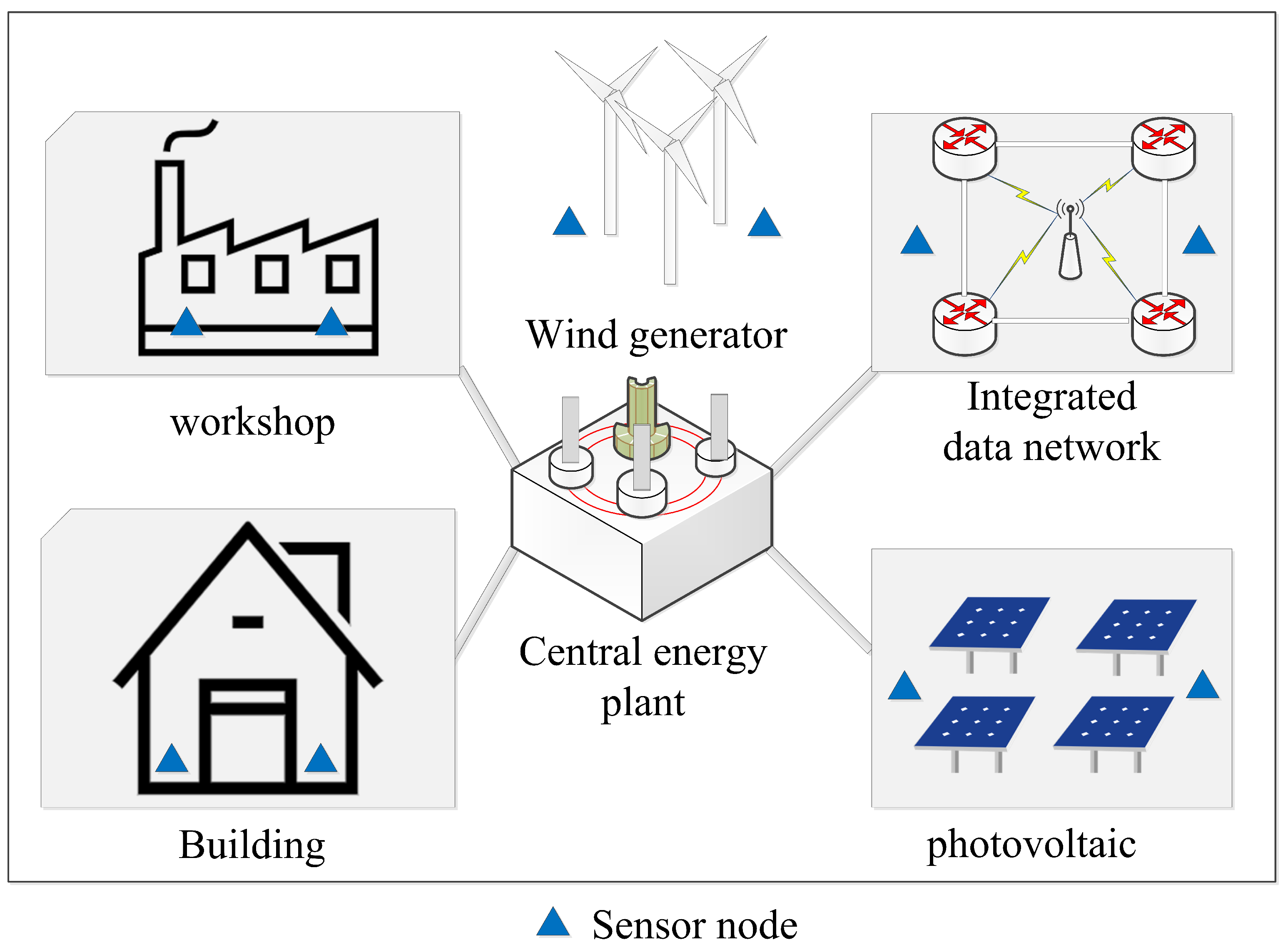
With the development of the power grid, the concept of microgrids came into being. The microgrids is placed at the end of the entire grid-connected system. The WSN is engaged in the management of power generation, power consumption, transmission and distribution. In terms of power generation, the WSN detects the power generated by the microgrid for large-scale applications. In addition, the WSN needs to monitor the transmission status of the microgrid to transmit power effectively. However, the energy of sensor nodes is limited. Under the condition of limited energy, how to improve the efficiency of data transmission and the lifetime of the sensor network is a crucial concern.

A three-layer framework is proposed based on joint rate-aware fuzzy clustering and stable sensor association that considers various factors of sensor energy efficiency [10]. In [11], fog computing was utilized to optimize the WSN connected to the microgrid. In the grid-connected community (GCC), an energy model was modeled to evaluate the energy consumption of the WSN and its performance in microgrids. The collected information of sensor nodes is used to calculate the optimal value of data transmission by utilizing the whale optimization algorithm, which reduces the energy consumption of the sensor network and improves the throughput of the network. In [12], a load balancing and routing strategy using the Glowworm swarm optimization approach (LBR-GSO) is adopted to handle the energy consumption of sensor nodes.

In the WSN, the CHs consume more energy than other nodes, so the lifetime of the CHs is shorter than other cluster members (CMs). Therefore, to extend the sensor network’s lifetime, the load of the sensor nodes connected to the CHs must be balanced. This is the load balancing clustering problem, which is an NP-hard. In [13], a routing algorithm was proposed. The routing algorithm reduces and balances the energy consumption in the network by finding a suitable path between each CH and the aggregation end. In [14], a user association and resource allocation algorithm was investigated based on the Stackelberg game. In [15], a distributed WSN scheme based on grid clustering and fuzzy reinforcement learning was proposed to maximize the network life cycle while achieving energy-efficient data aggregation. In [16], path operator calculus centrality was utilized to optimize the centrality problem in routing, the harmony search algorithm was used to find the main routing path, and then the particle swarm algorithm was used to estimate high centrality nodes. At last, optimal routing with reduced energy consumption was found. As a result, the hybrid algorithm reduced time delay and increased residual energy, effectively balancing energy consumption.

Considering that different transmission protocols have an impact on the energy consumption of sensor nodes. It is a challenging task to implement complex service quality protocols and security mechanisms in sensor networks. In addition, the WSN should not only focus on reducing the power consumption of sensor devices but also maintain the high reliability and high throughput required for smart grids applications [17]. In [18], a new data acquisition routing scheme was proposed based on bionic self-optimizing butterfly matching optimization, a self-optimizing intelligent routing protocol. In [19], an "Efficient Power Grid Link Routing Protocol" was proposed in WSN to expand the network’s lifetime. First, the grid algorithm was utilized to divide the nodes into virtual units, and then the intra-cluster and inter-cluster chains are used for data transmission, and each node communicates with its neighboring nodes. The protocol can improve the stability of the network and reduce energy consumption more than the low-energy adaptive clustering hierarchy (LEACH) protocol.

In addition, area coverage is also a crucial issue in WSN, and it will impact the perceived quality of the target area, namely, the coverage of non-penetrating obstacles in the microgrids where sensors cannot be deployed or sensor signals cannot pass through. The target coverage area is discretized in the deployment diagram representation of impenetrable obstacles. In [20], a probabilistic detection model was utilized to represent sensors with variable distance coverage. The area coverage problem was formulated as a mixed-integer nonlinear programming problem, which was solved by an iterative process.

3. System Model

In this section, we describe the system model. As shown in Figure 1, we consider a microgrids system based on a smart factory. The system includes five types of facilities: a workshop, a central energy plant, a wind generator, an integrated data network, photovoltaics and offices. New energy facilities such as wind generators and photovoltaics intermittently generate electricity to reduce the impact on the center-dependence of the grid. To ensure the stable operation of the entire microgrid system, a WSN consisting of N sensors is deployed. The set of sensors are denoted as $\mathcal{N}$, where $\left|\mathcal{N}\right|=N$. Due to the randomness of the deployment location in the practical scene, all sensor nodes are deployed through the Poisson point process ($\mathrm{PPP}$) with a density of $\rho$ in this paper, including temperature, voltage, current, light intensity and wind speed, etc., which presents a relatively random sensor deployment to cover more application scenarios. Of course, wind speed sensors and light intensity sensors are mainly deployed near wind generators and photovoltaics, respectively, in actual scenarios. In order to obtain effective topology control, all sensor nodes are divided into K clusters. The sensor nodes in each cluster will select one of them to become the CH, and the other sensor nodes will become CMs. The set of CHs are denoted as $\mathcal{K}$, where $\left|\mathcal{K}\right|=K$ and $\mathcal{Z}=\left\{{\mathcal{Z}}_1,\cdots {\mathcal{Z}}_j,\cdots ,{\mathcal{Z}}_K\right\}$, ${\sum }_{m\in \mathcal{K}}\left|{\mathcal{Z}}_m\right|=N-K$. The CMs collect data and transmit it to the CH. The CH is responsible for collecting the data from the CMs and transmitting them to the BS via the uplink channel after fusion. Therefore, we have the following assumptions for the entire WSN. First, once the sensor is deployed, the location will no longer change. Secondly, all sensors are homogeneous and have the same data processing capacity and energy consumption model, but the size of the data packets generated by each sensor in each round is different, which is related to the data acquisition time. Finally, all sensors contain the same initial energy, and the energy of the data transmission gradually decreases. When the energy is exhausted, the node is considered to be dead.

Energy Consumption Model

The sensor operating time is mainly divided into two parts. The first part is data acquisition. At this stage, each sensor collects a certain bit of data and waits to be transmitted to the CH; the second part is the data transmission and reception stage, the CMs upload the collected data through the wireless channel, and CH receives the data and processes data from CMs.

In the data acquisition stage, the energy consumption of the sensor node n can be expressed as follows:

$$E_{n,c}=p_c*t_n,$$

(1)

where $p_c$ is the acquisition power, and $t_n$ is the acquisition time of sensor node n. In addition, the longer the acquisition time of the sensor, the smaller the probability of data distortion and the higher the satisfaction level that can be obtained. Therefore, the satisfaction level of sensor node n can be defined as the utility function of time t:

$$\sigma U_n\left(t_n\right),$$

(2)

where $\sigma >0$ is a coefficient of the satisfaction function. The utility function is a monotonic increasing function of time $t_n$. This function can be modeled as a logarithmic function and is also used in [21,22]. Of course, the algorithm and simulation results presented in this paper can be easily implemented when sensor nodes have different utility functions. However, as the acquisition time of the sensor is longer, more amount of data are generated correspondingly. The maximum acquisition time of data is defined as $T_{max}$.

In the data transmission stage, the energy model in [23] was used. The energy model mainly includes two parts: transmission power consumption and circuit power consumption. In this paper, we introduce the transmission rate of the node into the energy model, because the bandwidth and SNR of the channel have a certain impact on the transmission energy consumption. So the energy consumption of sensor node n data transmission is as follows:

$$E_{n,t}=\frac{1}{\eta }(p_t+\alpha )*\frac{l*t_n}{r_n},$$

(3)

where $\eta$ is defined as the efficiency of the power amplifier, $p_t$ is the transmission power, $\alpha$ is the circuit power consumption of data transmission, $l>0$ is the amount of data acquisition per unit time and $r_n$ is the data transmission rate.

The energy consumption of the sensor node receiving acquisition data is expressed as follows:

$$E_{n,r}=e_c*l*t_n,$$

(4)

where $e_c$ is the circuit power for data reception. In addition, the CH receives data from all CMs. In order to reduce energy consumption, the received data need to be fused into $l·t_n$ and then transmitted to the BS. The energy consumption per bit of data fusion is denoted as $E_{DA}$.

According to the above energy model, the energy consumption of CHs and CMs in each round can be obtained. $x_{ij}$ is denoted as $x_{ij}\in \{0,1\}$ as a binary variable, which represents the association status of CM i, where $i\in \mathcal{L}$ and $j\in \mathcal{K}$. If $x_{ij}=1$, this means that the CM i chooses to access the CH j, otherwise $x_{ij}=0$. Then, the following constraints need to be added:

$$\begin{array}{cc}\hfill & \sum _j{x}_{ij}=1,\forall i\in \mathcal{L},\hfill \end{array}$$

(5)

$$\begin{array}{cc}\hfill & \sum _i{x}_{ij}\le N_j^{max},\forall j\in \mathcal{K},\hfill \end{array}$$

(6)

$$\begin{array}{cc}\hfill & x_{ij}\in \{0,1\},\forall i\in \mathcal{L},j\in \mathcal{K},\hfill \end{array}$$

(7)

where $N_j^{max}$ is the maximum number of CMs that CH j can access. Consequently, the energy consumption of CM i in each round can be expressed as follows:

$$E_{C{M}_i}=\frac{1}{\eta }(p_t+\alpha )*l*t_i\sum _j\frac{x_{ij}}{r_{ij}}$$

(8)

where $r_{ij}$ is the transmission rate from CM i to CH j.

The energy consumption of each CH includes three parts: receiving data from CMs, data fusion and sending data to the BS. The energy consumption of the CH j in each round can be expressed as follows:

$$E_{C{H}_j}=e_c*\sum _i(l*t_i*x_{ij})+E_{DA}*\left(\sum _i(l*t_i*x_{ij})+l*t_j\right)+\frac{1}{\eta }(p_t+\alpha )\frac{l*t_j}{r_{con}},$$

(9)

where $r_{con}$ is the transmission rate between the CHs and the BS. Since the location of the BS is fixed, the CHs have been determined by the CHs selection algorithm, $r_{con}$ is a constant.

4. Problem Formulation and Problem Solution

In order to reduce the WSN’s energy consumption and extend its lifetime, the topology control of the WSN needs to be considered. The topology control generally includes two parts: sensor association and CHs selection, which only considers the data transmission phase of the WSN. Based on the existing work, in order to optimize the energy consumption of sensor nodes during the entire working phase, this paper considers the following three issues: acquisition time design, CHs selection and sensor association. First, the CHs are selected based on the CHs selection algorithm. Then, a multi-constrained mixed integer optimization problem of joint acquisition time design and sensor association is formulated. By solving this optimization problem, the current acquisition time and the sensor association under the current CHs can be determined. After that, select the CHs again and repeat this process until the CHs, acquisition time and sensor associations do not change. At this time, we think that a high-quality sub-optimal solution has been obtained. Of course, since the initial acquisition time and sensor association are unknown, at the beginning of the iteration, we randomly select K sensor nodes as CHs and the remaining nodes automatically become CMs.

4.1. Cluster Heads Selection

According to the energy model used in this paper, to minimize the energy consumption of the entire WSN, the CHs should be located in the center of the entire cluster. Therefore, we choose the sensor node, which has the smallest sum of Euclidean distances with other sensor nodes in the same cluster as the CHs in this paper. Other sensor nodes automatically become CMs, and the specific formula for CHs selection is shown in the following formula:

$$C{H}_j=arg\underset{q}{min}\left\{\sum dis{t}_{q,{\mathbb{Z}}_m},\forall q\in {\mathcal{Z}}_m\right\},\forall j\in \mathcal{K},$$

(10)

where ${\mathbb{Z}}_m$ represents the set of ${\mathcal{Z}}_m$ that removes the node q. $\sum dis{t}_{q,{\mathbb{Z}}_m}$ is the sum of the distances from node q to other nodes in the cluster.

4.2. Problem Formulation

In the previous part, we have selected the CHs by Equation (10). In this part, a joint optimization problem of the acquisition time $\mathit{T}=\{t_n,n\in \mathcal{N}\}$ and the sensor association $\mathit{X}=\{x_{ij},i\in \mathcal{L},j\in \mathcal{K}\}$ is formulated based on the result of the CHs selection. In order to improve the satisfaction of sensor data acquisition, reduce the energy consumption of the WSN and ensure the stable operation of the microgrids, we jointly optimize the acquisition time $\mathit{T}$ and sensor association $\mathit{X}$ to maximize data satisfaction and minimize the energy consumption of each round of WSN. Therefore, this paper constructs an optimization problem as follows:

$$\begin{array}{cc}\hfill \mathbf{P}:\underset{\mathit{T},\mathit{X}}{max}& \sum _{n}U\left(t_n\right)-\beta \left(p_c\sum _n{t}_n+\sum _i{E}_{C{M}_i}+\sum _j{E}_{C{H}_j}\right)\hfill \\ \hfill s.t.& \sum _j{x}_{ij}=1,\forall i\in \mathcal{L},\hfill \\ \hfill & \sum _i{x}_{ij}\le N_j^{max},\forall j\in \mathcal{K}\hfill \\ \hfill & x_{ij}\in \{0,1\},\forall i\in \mathcal{L},\forall j\in \mathcal{K}\hfill \\ \hfill & 0\le t_n\le T_{max},\forall n\in \mathcal{N}\hfill \end{array}$$

(11)

where $\beta >0$ is the trade-off between satisfaction and energy consumption. First and third constraints ensure the association of a single CH and the maximum number of CMs that the CH can access are restricted through second constraint. Since the $x_{ij}$ are binary variables, the optimization problem $\mathbf{P}$ is a multi-constrained mixed-integer programming problem. However, the mixed-integer programming problem is generally challenging to obtain the optimal solution. If the brute force algorithm is used to obtain it, the algorithm complexity is extremely high. Furthermore, it is still challenging to obtain the optimal solution when the dimensionality of the optimization problem is high.

4.3. Problem Solution

For problem $\mathbf{P}$, we use the BCD algorithm [24] to solve the original problem by dividing it into two sub-problems, namely, the acquisition time $\mathit{T}$ and the sensor association $\mathit{X}$. Then, in each iteration, two sub-problems are solved in turn. When the iteration reaches the prescribed accuracy, we think that the sub-optimal solution of the optimization problem $\mathbf{P}$ has been obtained.

4.3.1. Acquisition Time Optimization

We first optimize the acquisition time $\mathit{T}$ with given sensor association $\mathit{X}$. At this time, the optimization problem $\mathbf{P}$ can be expressed as follows:

$$\begin{array}{cc}\hfill \mathbf{P}\mathbf{1}:\underset{\mathit{T}}{max}& \sum _{n}U\left(t_n\right)-\beta \left(p_c\sum _n{t}_n+\sum _i{E}_{C{M}_i}+\sum _j{E}_{C{H}_j}\right)\hfill \\ \hfill & =\sum _{n}U\left(t_n\right)-\beta \left(p_c\sum _n{t}_n+\sum _i\left[\frac{1}{\eta }(p_t+\alpha )*l*t_i*\sum _j\frac{x_{ij}}{r_{ij}}\right]\right.\hfill \\ \hfill & \left.+\sum _j\left[e_c*\sum _i(l*t_i*x_{ij})+E_{DA}*(\sum _i(l*t_i*x_{ij})+l*t_j)\right]\right)\hfill \\ \hfill s.t.& 0<t_n<T_{max},\forall n\in \mathcal{N}.\hfill \end{array}$$

(12)

It can be seen that when the satisfaction function $U(·)$ is modeled as a convex function, the problem is a convex optimization problem about $\mathit{T}$, so the strong duality condition holds. Therefore, its Lagrangian function and dual problem can be constructed as follows:   

$$\begin{array}{cc}\hfill L(\mathit{T},\lambda ,\nu )& =\sum _{n}U\left(t_n\right)-\beta \left(p_c\sum _n{t}_n+\sum _i\left[\frac{1}{\eta }\left(p_t+\alpha \right)*l*t_i*\sum _j\frac{x_{ij}}{r_{ij}}\right]+\sum _j\left[e_c*\sum _i(l*t_i*x_{ij})\right.\right.\hfill \\ \hfill & \left.\left.+E_{DA}*(\sum _i(l*t_i*x_{ij})+l*t_j)\right]\right)+\sum _n{\lambda }_n{t}_n+\sum _n{\nu }_n(T_{max}-t_n),\hfill \end{array}$$

(13)

where $\lambda =\{{\lambda }_n,\forall n\in \mathcal{N}\},\nu =\{{\nu }_n,\forall n\in \mathcal{N}\}$ is a non-negative Lagrangian multiplier. Then the dual function is expressed as follows:

$$D(\lambda ,\nu )=\underset{\mathit{T}}{max}L(\mathit{T},\lambda ,\nu ).$$

(14)

The dual problem is as follows:

$$\begin{array}{cc}\hfill \underset{\lambda ,\nu }{min}& D(\lambda ,\nu )\hfill \\ \hfill s.t.& \lambda ⪰0,\hfill \\ \hfill & \nu ⪰0.\hfill \end{array}$$

(15)

In order to obtain the dual function, we take the first derivative of the Lagrangian function with respect to $\mathit{T}$ to obtain:

$$\begin{array}{c}\hfill \begin{array}{c}\hfill t_n^{*}=\left\{\begin{array}{c}{U}^{\prime -1}\left[\beta \left(p_c+\frac{(p_t+\alpha )l}{\eta }*\sum _j\frac{x_{ij}}{r_{ij}}+l(e_c+E_{DA})\sum _j{x}_{ij}\right)-{\lambda }_n+{\nu }_n\right],ifn\in \mathcal{L},\hfill \\ U^{\prime -1}\left[\beta (p_c+l)-{\lambda }_n+{\nu }_n\right],ifn\in \mathcal{K},\hfill \end{array}\right.\end{array}\end{array}$$

(16)

when $t_n^{*}$ is found, and the dual function can be obtained. Then, we can solve the dual problem to obtain the optimal solution of $\mathbf{P}\mathbf{1}$. For the dual problem, we use the sub-gradient method to obtain the optimal Lagrangian multiplier. The iterative expression is as follows:

$${\lambda }_n^{(r+1)}={[{\lambda }_n^r+s_r{t}_n]}^{+},\forall n\in \mathcal{N},$$

(17)

$${\nu }_n^{(r+1)}={[{\nu }_n^r+s_r(T_{max}-t_n)]}^{+},\forall n\in \mathcal{N},$$

(18)

where ${\left[x\right]}^{+}\triangleq max\{x,0\}$, $s_r$ is the r-th iteration step, and its value is set to $s_r=\beta /\parallel g^r\parallel$; $g^r$ is the current gradient of the dual function for the r-th iteration. The details of subgradient iteration can be seen from algorithm ATSAO.

4.3.2. Sensor Association Optimization

When the acquisition time $\mathit{T}$ is given, the optimization problem of sensor association $\mathit{X}$ at this time can be expressed as follows:   

$$\begin{array}{cc}\hfill \mathbf{P}\mathbf{2}:& \underset{\mathit{X}}{min}\sum _i{E}_{C{M}_i}+\sum _j{E}_{C{H}_j}\hfill \\ \hfill & =\sum _i\left[\frac{1}{\eta }(p_t+\alpha )*l*t_i*\sum _j\frac{x_{ij}}{r_{ij}}\right]+\sum _j\left[e_c*\sum _i(l*t_i*x_{ij})+E_{DA}*\left(\sum _i(l*t_i*x_{ij})\right)\right]\hfill \\ \hfill s.t.& \sum _j{x}_{ij}=1,\forall i\in \mathcal{L},\hfill \\ \hfill & \sum _i{x}_{ij}\le N_j^{max},\forall j\in \mathcal{K},\hfill \\ \hfill & x_{ij}\in \{0,1\},\forall i\in \mathcal{L},\forall j\in \mathcal{K}.\hfill \end{array}$$

(19)

Problem $\mathbf{P}\mathbf{2}$ is a 0–1 multi-knapsack problem. Dynamic programming is widely used to solve the knapsack problem, but when the dimensionality of the problem to be solved is very large, the solution efficiency of dynamic programming will be drastically reduced, which is called the dimensionality disaster.

Based on the above description, we propose an approximate solution for problem $\mathbf{P}\mathbf{2}$ to obtain the sensor association $\mathit{X}$ based on the method in [25]. This method iteratively considers all objects that are not loaded into the backpack and calculates the Euclidean distance between the optimal and suboptimal returns each time. The object corresponding to the maximum Euclidean distance will be loaded into the backpack in this iteration until all objects are loaded into the backpack, at which time the algorithm stops iterating. See the detailed algorithm ATSAO, where $w_{ij}$ is a measure of the “desirability” of assigning the item i to knapsack j. From question $\mathbf{P}\mathbf{2}$, $w_{ij}$ can be calculated by the following formula, which can be derived by Equation (19):

$$w_{ij}=\sum _i\sum _j\left(\frac{\frac{1}{\eta }(p_t+\alpha )*l*t_i}{r_{ij}}+(e_c+E_{DA})*l*t_i\right).$$

(20)

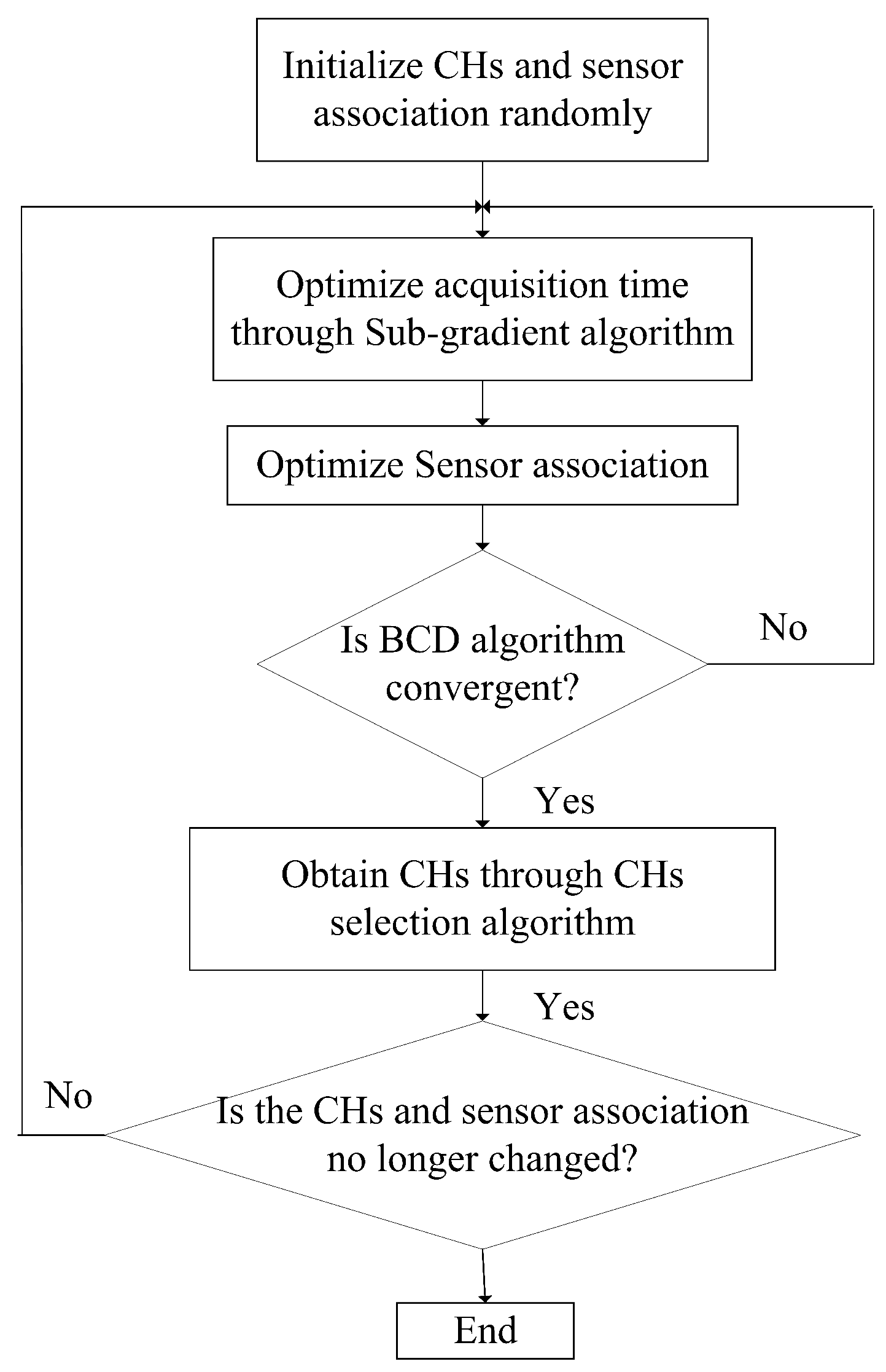
4.4. Overall Algorithm Design

Based on the previous description, we propose a total iterative Algorithm 1 to obtain the acquisition time $\mathit{T}$ and sensor associations $\mathit{X}$ to solve the problem effectively with low computational complexity. First, the CHs, sensor association $\mathit{X}$ and Lagrangian multipliers $\{\lambda ,\nu \}$ are randomly initialized, and then the acquisition time $\mathit{T}$ from steps 6 to 9 is obtained through multiple iterations of the sub-gradient algorithm, until the sub-gradient algorithm converges to the specified accuracy. We can solve the problem $\mathbf{P}\mathbf{2}$ and obtain the sub-optimal sensor association $\mathit{X}$ based on above description from steps 10 to 22. In the process of solving this problem, $w_{ij}$ needs to be calculated. It represents the price of the knapsack problem. Then, we iteratively consider all CMs. When all CMs are associated with the CHs, the sensor association $\mathit{X}$ is obtained. As for the problem $\mathbf{P}$, we use multiple iterations to find its solution. By applying the BCD method, the process of obtaining the acquisition time $\mathit{T}$ and the sensor association $\mathit{X}$ requires multiple iterations to obtain a sub-optimal solution. Finally, the CHs are selected based on the sensor association result according to the CHs selection algorithm from steps 25 to 26. Of course, the CHs selection and acquisition time $\mathit{T}$ and sensor association $\mathit{X}$ also need to be iterated many times until the CH and $\mathit{X}$ no longer change. This is because the CHs are randomly initialized during initialization, and a high-quality topology control strategy can be obtained after multiple iterations. Finally, after a finite number of iterations when the algorithm converges to the predetermined accuracy, we believe that the problem $\mathbf{P}$ is successfully solved. The details of the algorithm are summarized as algorithm ATSAO.

Figure 2 shows the flowchart of the ATSAO algorithm. Firstly, CHs and sensor association are initialized randomly. Secondly, the BCD algorithm is used to solve the optimization problem formulated in this paper. In each iteration, the acquisition time is optimized through the Lagrangian dual method under the given sensor association. The sensor association is optimized based on the optimization results of acquisition time. When the change of the optimization objective function is below a predefined threshold, it shows that the BCD algorithm converges. After that, a low-complexity CH selection algorithm is proposed to obtain the CHs. After the CHs and sensor association are no longer changed, the algorithm ATSAO converges.

In the system model of this paper, we assume that there are K CHs and $N-K$ CMs in the WSN, and the number of CMs in each cluster is $|{\mathcal{Z}}_1|,\cdots ,|{\mathcal{Z}}_K|$. In the ATSAO, the algorithm complexity involved in solving the problem $P2$ is $o(K{(N-K)}^2)$, the complexity of CHs selection algorithm is $o\left(K\right(|{\mathcal{Z}}_1{|}^2+|{\mathcal{Z}}_2{|}^2+\cdots +|{\mathcal{Z}}_k{|}^2\left)\right)$. Due to $|{\mathcal{Z}}_1{|}^2+|{\mathcal{Z}}_2{|}^2+\cdots +{\left|{\mathcal{Z}}_k\right|}^2\le {\left(|{\mathcal{Z}}_1|+|{\mathcal{Z}}_2|+\cdots +|{\mathcal{Z}}_k|\right)}^2$ and ${\left(|{\mathcal{Z}}_1|+|{\mathcal{Z}}_2|+\cdots +|{\mathcal{Z}}_k|\right)}^2={\left(N-K\right)}^2$, the total algorithm complexity is $o(K{(N-K)}^2)$. If the problem $P2$ is solved by GREEDY algorithm, its complexity is $o\left(K\right(N-K\left)\right)$.

Algorithm 1 Acquisition Time and Sensor Association Optimization (ATSAO).

1: Initialize CHs and sensor association $X^0$ randomly. 2: Initialize ${(\lambda ,\nu )}^1$ and $r_1,r_2,r_3=0$. 3: repeat 4:     repeat 5:         repeat 6:            Update $T^{r_1}$ according to Equation (16). 7:            Update ${(\lambda ,\nu )}^{r_1+1}$ according to Equations (17) and (18), respectively. 8:            Update $r_1=r_1+1$. 9:         until Sub-gradient algorithm converges to a prescribed accuracy. 10:         Calculate $w_{ij}$ according to Equation (20). 11:         while $\mathcal{L}\ne \oslash$ do 12:            $d^{*}=-\infty$. 13:            for each node $i\in \mathcal{L}$ do 14:                $j^{\prime }=arg\underset{j}{max}\{w_{ij},\forall i\in \mathcal{L}\}$. 15:                Calculate $d=w_{i{j}^{\prime }}-max\{w_{ij},\forall j\in \mathcal{K}\}$. 16:                if $d>d^{*}$ then 17:                    $d^{*}=d$. 18:                    $x_{i{j}^{\prime }}=1$. 19:                end if 20:            end for 21:            Remove node i from $\mathcal{L}$. 22:         end while 23:         Update $r_2=r_2+1$. 24:     until The increase in the objective value is below a threshold, i.e., the convergence of BCD algorithm. 25:     Obtain the CHs through CHs selection algorithm. 26:     Update $r_3=r_3+1$. 27: until CHs and sensor association $\mathit{X}$ no longer change.

In addition, in order to obtain the lower bound of the problem $\mathbf{P}\mathbf{2}$, we use a GREEDY algorithm with relatively low computation complexity. The GREEDY algorithm makes the best choice based on the current situation at each step, regardless of the global situation, which dramatically reduces the computation resource required to obtain the optimal solution. However, the GREEDY algorithm is proven to have a particular gap between the solution obtained when solving the 0–1 knapsack problem and the optimal solution. In this paper, we will compare the performance gap with other algorithms.

In order to obtain the upper bound of the problem $\mathbf{P}\mathbf{2}$, we first relax the problem $\mathbf{P}\mathbf{2}$. After the relaxation, the problem is as follows:

$$\begin{array}{cc}\hfill \mathbf{P}\mathbf{2}.\mathbf{1}& \underset{\mathit{X}}{min}\sum _i{E}_{C{M}_i}+\sum _j{E}_{C{H}_j}\hfill \\ \hfill =& \sum _i\left[\frac{1}{\eta }(p_t+\alpha )*l*t_i\sum _j\frac{x_{ij}}{r_{ij}}\right]+\sum _j\left[e_c*\sum _i(l*t_i*x_{ij})+E_{DA}*(\sum _i(l*t_i*x_{ij}))\right]\hfill \\ \hfill s.t.& \sum _j{x}_{ij}=1,\forall i\in \mathcal{L},\hfill \\ \hfill & \sum _i{x}_{ij}\le N_j^{max},\forall j\in \mathcal{K},\hfill \\ \hfill & 0\le x_{ij}\le 1,\forall i\in \mathcal{L},\forall j\in \mathcal{K}.\hfill \end{array}$$

(21)

The objective function and constraints of the problem $\mathbf{P}\mathbf{2}.\mathbf{1}$ are affine. Therefore, it is a linear programming problem and can be directly solved through the CVX toolbox. The sensor association $\mathit{X}$ is obtained as a continuous variable between 0 and 1, which means that a single CM allows the association of multiple CHs, i.e., “fraction sensor association (FSA)”. This relaxation reduces the complexity of the problem and makes it no longer a combinatorial problem. Therefore, the optimal sensor association $\mathit{X}$ is successfully found and the upper bound of the problem $\mathbf{P}\mathbf{2}$ has also been obtained through relaxation.

A lower bound of the problem $\mathbf{P}\mathbf{2}$ is obtained by the GREEDY algorithm, and its upper bound is obtained by the relaxation method. They can replace steps 10 to 22 in algorithm ATSAO, and the difference in performance is also shown in the simulation results section.

5. Experiment Simulation

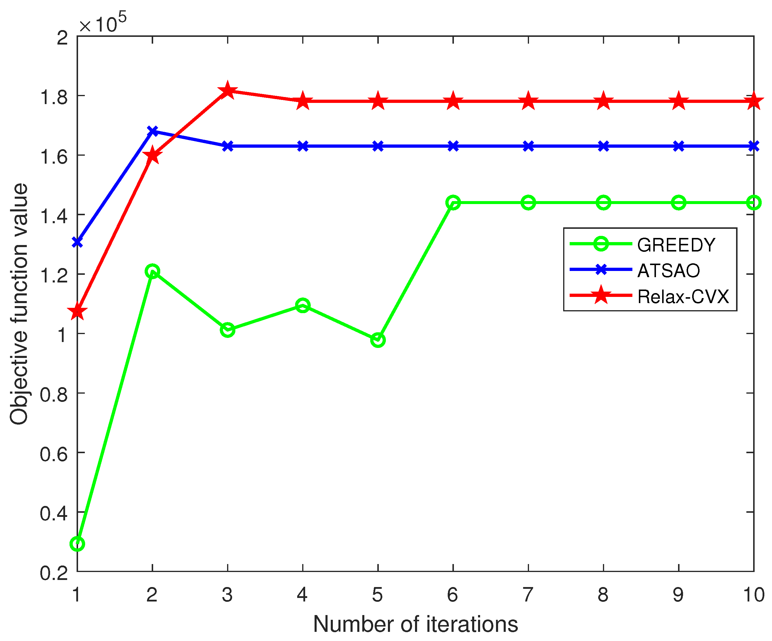
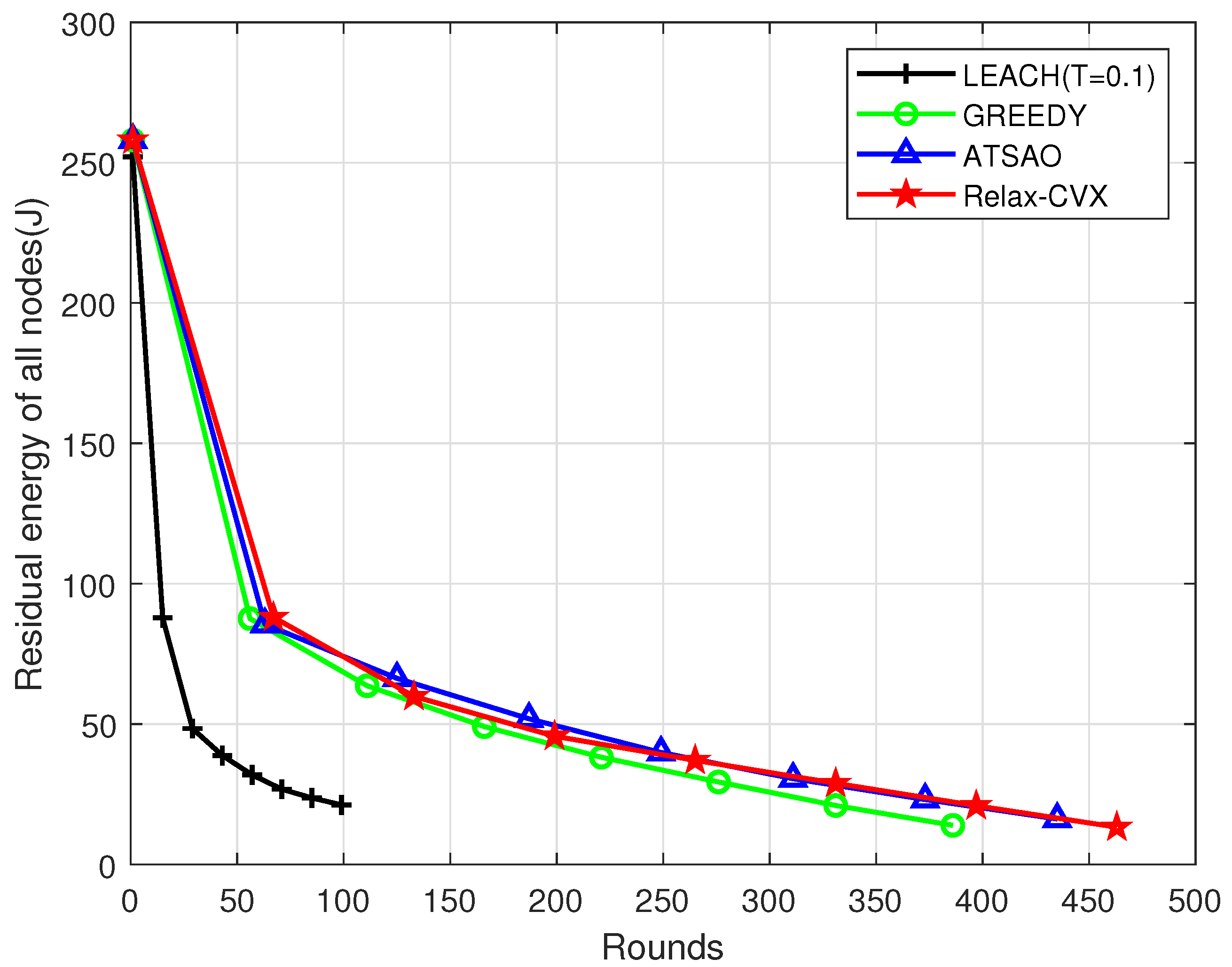
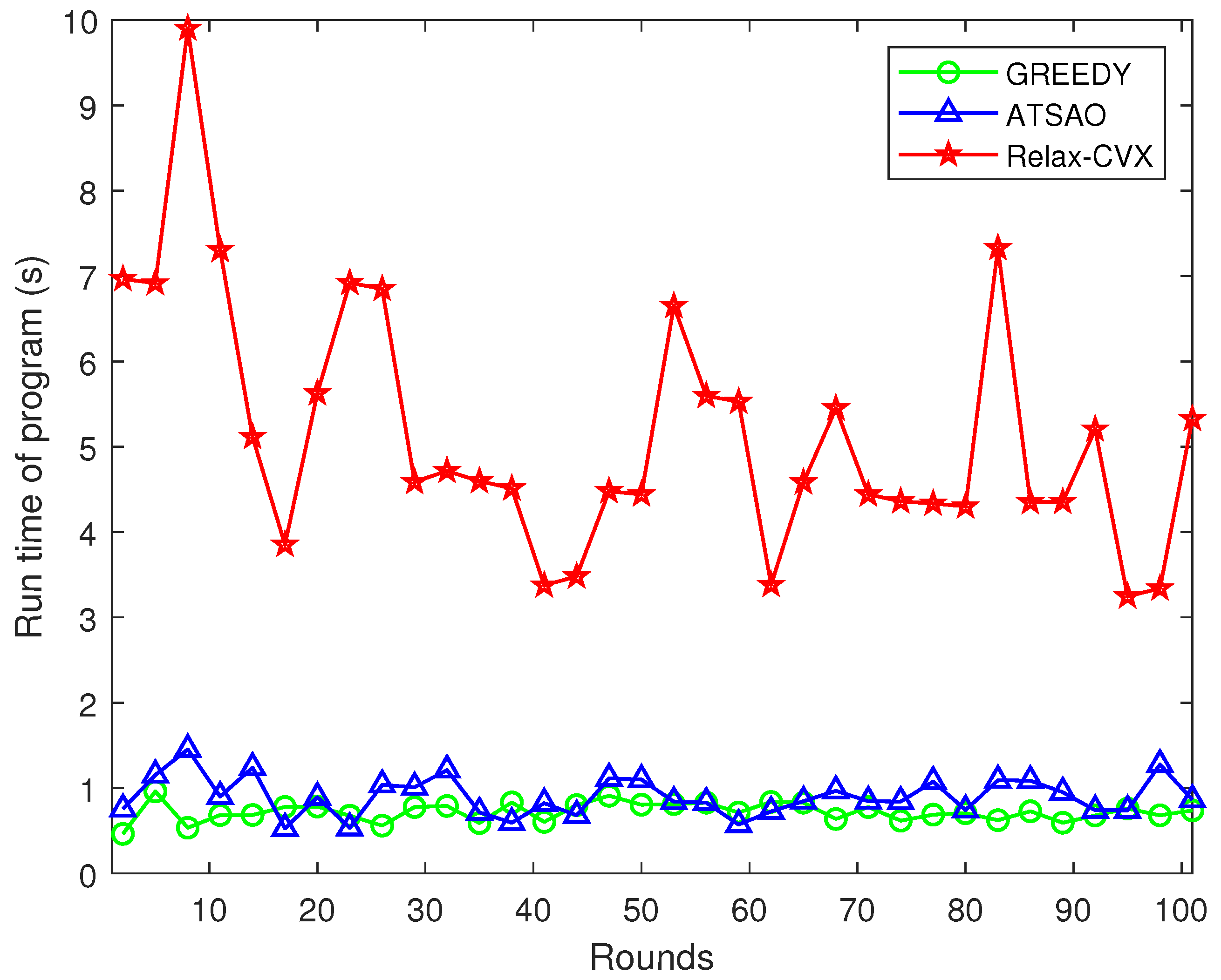
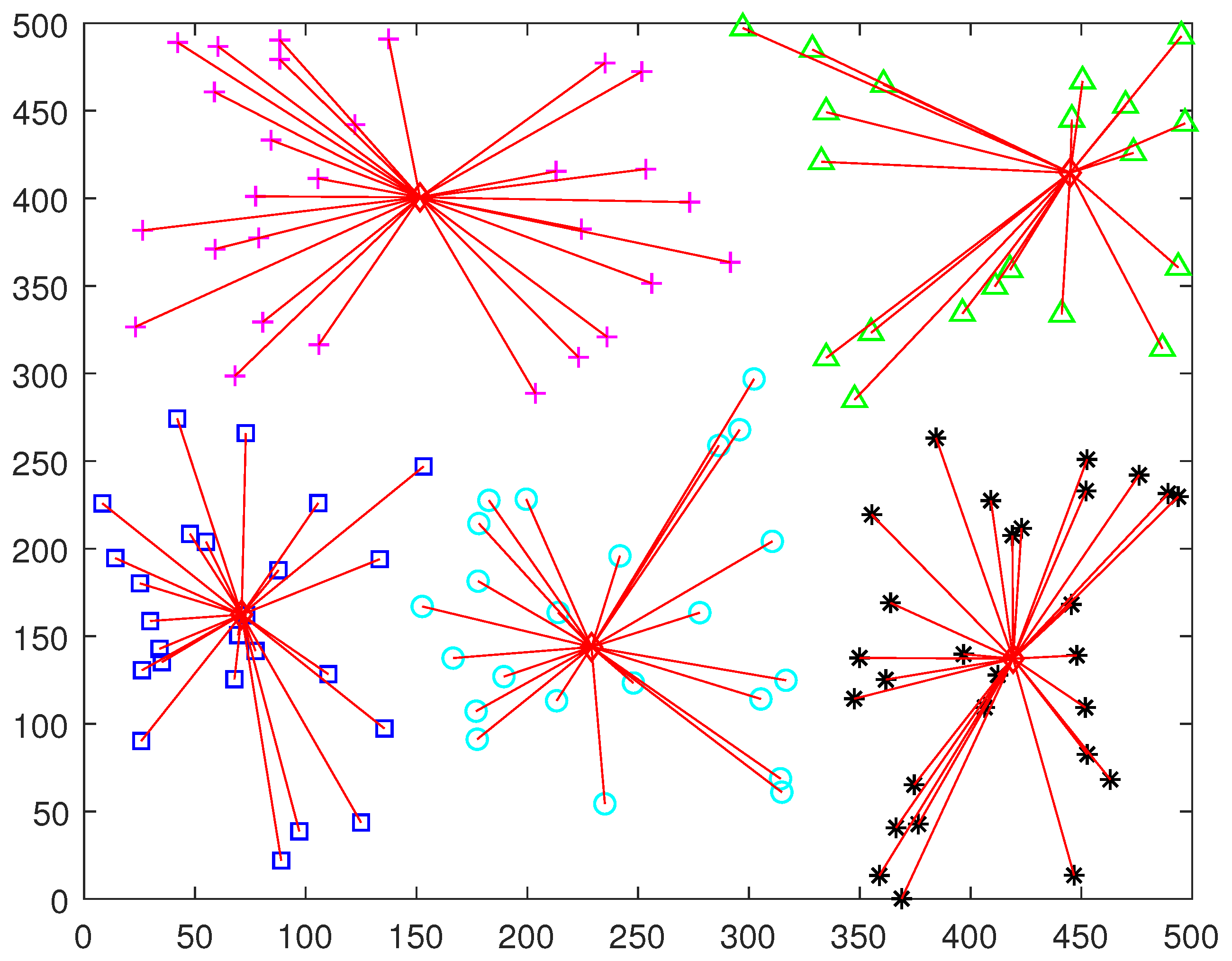
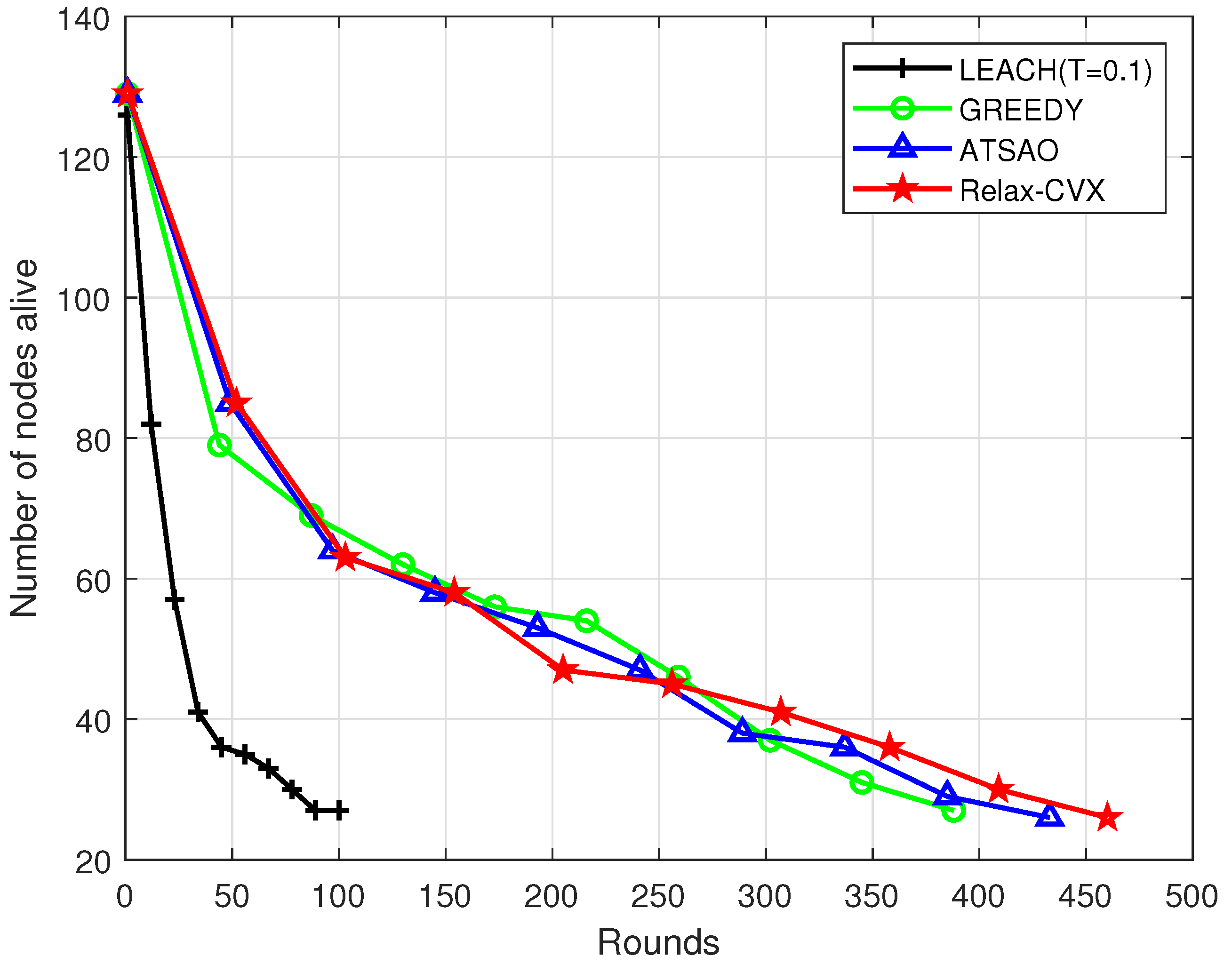
In this part, we will demonstrate the effectiveness of the algorithm proposed in this paper through simulation. We consider a WSN, where N sensor nodes are deployed on a square area with an area of S, and the base station is located in the center of the network. The path loss between CMs and CH and between CH and BS is modeled as $L\left(d\right)=34+40logd$, where $d>0$ indicates the Euclidean distance from the CH to the BS and from CMs to the CH; it is also used in [26]. According to the different methods used to obtain the user association in the second subsection, we will mark the three algorithms proposed in this paper as GREEDY, ATSAO and Relax-CVX and compare them with the classic topology control algorithm LEACH proposed in [27]. Since the classic LEACH algorithm only considers the topology control, and does not consider the acquisition energy consumption of sensor nodes. Therefore, we set the acquisition time of LEACH to T in simulations of this paper. It is obvious that the value of T has a great impact on the algorithm simulation results. In the simulation of this paper, we find that the optimal value of acquisition time $t^{*}$ is between 0.01 s and 1 s. Therefore, the value of T is set to 0.1 s. It is worth noting that the acquisition time T is designed only to explore the performance of the algorithm not to be close to a certain standard. The simulation parameters used in this paper are shown in

Table 1. Simulation parameters.

Variable	Parameter	Value
S	Distribution area	$500\times 500$
$\rho$	Deployment density of WSN nodes	250
$N_j^{max}$	Maximum access number of CH	30
$\sigma$	Satisfaction coefficient	$1\times {10}^3$
l	Amount of data generated per unit time	40 bit
$\beta$	Trade-off parameter	100
$p_c$	Data acquisition power	1 mW
$p_t$	Data transmission power	20 mW
$\eta$	Power amplifier efficiency	0.9
$\alpha$	Circuit power	5 mW
$e_c$	Energy consumption for data receiving	5 nJ/bit
$E_{DA}$	Energy cost for data aggregation	0.5 nJ/bit
$T_{max}$	Maximum acquisition time	10 s

. The performance evaluation is operated in Matlab 2020b. All the simulations are performed on a desktop with an Intel Core i7-7700 3.6 GHz CPU and 16 GB memory.

Simulation Results

Figure 3 shows the topology of the WSN and the results of the sensor association by the ATSAO during the first round. In this paper, the number of CHs is set to five. According to the CHs selection algorithm, the CHs are located in the center of the whole cluster, and other sensor nodes are associated with a single CH to transmit data.

Figure 4 shows the convergence performance of the algorithms proposed in this paper. It can be seen from the figure that as the number of iterations increases, the objective function value Equation (11) of the algorithms gradually increase. After about six iterations, all algorithms tend to convergence. At this time, the CHs and sensor associations no longer change. In addition, from the value of the objective function after the algorithms converge, it can be seen that the performance gap between the ATSAO proposed in this paper and the Relax-CVX is small. Compared with the GREEDY, the improvement is more significant when the complexity increase is not large.

Figure 5 shows that the residual energy changes of all sensor nodes versus number of iteration rounds. Compared with the LEACH, the algorithms proposed in this paper can effectively reduce the energy consumption of the entire WSN and prolong its lifetime. This is because energy consumption is considered when formulating the objective function of the optimization problem. The sensor association is obtained by solving the proposed optimization problem. Then, we select CHs according to the CHs selection algorithm, and multiple iterations have been carried out. Compared with the LEACH, the proposed algorithms in this paper can obtain a better topology control strategy and effectively reduce the transmission energy consumption of all sensor nodes. The Relax-CVX obtains the upper bound of the optimization problem by relaxing the knapsack problem. Therefore, it obtains the best performance. As for the ATSAO, the distance between the optimal gain and the sub-optimal gain is considered when selecting items to pack into the backpack. Compared with the GREEDY algorithm, which only considers the current optimal choice, the ATSAO can obtain better performance. Although compared to the Relax-CVX, the lifetime of the WSN network using the ATSAO is slightly reduced, the time complexity and computational complexity of the ATSAO are reduced significantly. Therefore, the ATSAO achieves a tradeoff between complexity and performance, which is meaningful for sensor nodes with limited computing capacity. The unreasonable CHs selection and sensor association of LEACH algorithm lead to the maximum energy consumption, and finally lead to the shortest lifetime of the WSN using the LEACH algorithm.

Figure 6 shows the change in the number of alive sensor nodes versus the neumber of iteration rounds. It can be seen that the algorithms proposed in this paper can slow down the death process of nodes. First, the Relax-CVX has the slowest death of sensor nodes, followed by the ATSAO, and the WSN with LEACH has the shortest lifetime. This is consistent with the relationship shown in Figure 3. It is because the slower the energy consumption of the sensor, the longer the node lifetime. Furthermore, the LEACH randomly selects nodes as CHs with a certain probability in each round. This seems to be able to delay the death process of the elected CH nodes. However, if the elected CHs are far from the cluster center, the transmission energy consumption of CMs will increase. Although randomly selecting CHs in each round can alleviate the energy hole problem, it will increase the energy consumption of the entire WSN, thereby shortening the lifetime.

Figure 7 shows that the data satisfaction per unit energy consumption of different algorithms. The greater the acquisition time, the higher the data satisfaction, but the corresponding energy consumption is also greater. Therefore, the data satisfaction per unit energy is calculated to represent the comprehensive performance of the algorithm, that is, to improve the data acquisition satisfaction as much as possible when the energy consumption is the same. It can be seen from the Figure 6 that the algorithm proposed in this paper can not only reduce the energy consumption of the WSN but also increases the satisfaction of data acquisition. When formulating the optimization problem, we aim to maximize the satisfaction of data collection and minimize the energy consumption of the whole network. Less transmission energy consumption contributes to greater data acquisition satisfaction in the acquisition stage. Therefore, similar to the trend of energy consumption, Relax-CVX obtained the highest data satisfaction, followed by the ATSAO.

Figure 8 shows the time consumed by different algorithms for each round, which reflects the complexity of the algorithms. It can be seen from Figure 8 that Realx-CVX consumes the most time per round, and the time consumed by the ATSAO in this paper is similar to that consumed by GREEDY. Compared with Relax-CVX, the time complexity of them is significantly reduced. Therefore, the ATSAO reduces the running time on the basis of ensuring the performance, which is of great significance for sensor nodes with limited energy.

6. Discussion

To reduce the energy consumption of the WSN for microgrid status detection, this paper considers the two stages of sensor acquisition and transmission, but most of the current work only considers the transmission stage [28,29]. Although the energy consumption of the acquisition stage is less than that of the transmission stage, such neglect does not achieve the minimum energy loss in reality. In this paper, when formulating the objective function of the optimization problem, the transmission energy consumption is taken into consideration. Finally, the sensor association with the best energy is obtained by solving the problem. In addition, for topology control, most of the current articles either select the CHs first and then associate the CMs, or select the CHs based on a result of clustering [30,31,32]. Few works try to obtain the optimal topology control strategy through multiple iterations. Considering that the initial clustering is generally not completely reasonable, and the CHs selected on this basis will not be energy-optimal, which is the necessity of multiple iterations. In this paper, the sensor association and the CHs selection are iterated many times until the CHs and sensor association no longer change. At this time, they are relatively considered to be optimal. In summary, this paper has made certain improvements based on existing work and theoretically can well improve the energy utilization efficiency of the WSN in the microgrid. The simulation results also show the effectiveness of the ATSAO proposed in this paper. Of course, since the main work of this article is to design the acquisition time and control sensor associations based on optimization problems, relatively few factors are considered in the selection of CHs. The limitations of this part will be improved in our future work.

7. Conclusions

To improve the monitoring quality and energy utilization efficiency of WSNs in microgrids, this paper proposes the ATSAO algorithm to design the acquisition time and perform topology control of WSN. First, the CHs are selected according to the CHs selection algorithm, and then the acquisition time and sensor association are obtained by an iterative algorithm based on BCD technology. Three methods of different complexity are used to obtain the sensor association. Finally, a sub-optimal acquisition time and topology control strategy are obtained. The simulation results show that the ATSAO can effectively reduce the energy consumption of the WSN and improve the satisfaction of data acquisition, thereby ensuring the power supply stability of the microgrids.

In the future, we will consider adding more practical constraints when formulating optimization problems to improve the performance of ATSAO. In addition, our current research is simulation-based, we will further implement real-time experiments.

References

1. Sharmila, N.; Nataraj, K.; Rekha, K. An Overview on Design and Control Schemes of Microgrid. In Proceedings of the 2019 Global Conference for Advancement in Technology (GCAT), Bangalore, India, 18–20 October 2019; pp. 1–4. [Google Scholar]
2. Kim, H.M.; Lim, Y. A communication framework in multiagent system for islanded microgrid. Int. J. Distrib. Sens. Netw. 2012, 8, 382316. [Google Scholar] [CrossRef]
3. Yang, H.; Zhang, J.; Qiu, J.; Zhang, S.; Lai, M.; Dong, Z.Y. A practical pricing approach to smart grid demand response based on load classification. IEEE Trans. Smart Grid 2016, 9, 179–190. [Google Scholar] [CrossRef]
4. Rana, M. Architecture of the internet of energy network: An application to smart grid communications. IEEE Access 2017, 5, 4704–4710. [Google Scholar] [CrossRef]
5. Swain, A.; Salkuti, S.R.; Swain, K. An Optimized and Decentralized Energy Provision System for Smart Cities. Energies 2021, 14, 1451. [Google Scholar] [CrossRef]
6. Kumar, S.; Singh, B.; Pal, B.C.; Xu, L.; Al-Durra, A. Energy efficient three-phase utility interactive residential microgrid with mode transfer capabilities at weak grid conditions. IEEE Trans. Ind. Appl. 2019, 55, 7082–7091. [Google Scholar] [CrossRef]
7. Lai, S.; Ravindran, B.; Cho, H. Heterogenous quorum-based wake-up scheduling in wireless sensor networks. IEEE Trans. Comput. 2010, 59, 1562–1575. [Google Scholar] [CrossRef]
8. Kumar, G.A.; Shivashankar; Sujay, N.; Tejas, P.; Srikanth, P.; Yashavanth, T. Design and implementation of wireless sensor network based smart DC grid for smart cities. In Proceedings of the 2019 4th International Conference on Recent Trends on Electronics, Information, Communication & Technology (RTEICT), Bengaluru, India, 17–18 May 2019; pp. 1453–1458. [Google Scholar]
9. Takriti, M.; Boussaada, Z.; Sansa, I.; Curea, O.; Bellaaj, N.M. Wireless Sensors Networks Applications For Micro-Grids Management: State of Art. In Proceedings of the 2020 6th IEEE International Energy Conference (ENERGYCon), Tunis, Tunisia, 28 September–1 October 2020; pp. 1058–1061. [Google Scholar]
10. Zhong, L.; Ge, M.; Zhang, S.; Liu, Y. Rate Aware Fuzzy Clustering and Stable Sensor Association for Load Balancing in WSNs. IEEE Internet Things J. 2021, 1. [Google Scholar] [CrossRef]
11. Karthik, S.S.; Kavithamani, A. Fog computing-based deep learning model for optimization of microgrid-connected WSN with load balancing. Wirel. Netw. 2021, 27, 2719–2727. [Google Scholar] [CrossRef]
12. Sampathkumar, A.; Mulerikkal, J.; Sivaram, M. Glowworm swarm optimization for effectual load balancing and routing strategies in wireless sensor networks. Wirel. Netw. 2020, 26, 4227–4238. [Google Scholar] [CrossRef]
13. Yarinezhad, R.; Hashemi, S.N. Solving the load balanced clustering and routing problems in WSNs with an fpt-approximation algorithm and a grid structure. Pervasive Mobile Comput. 2019, 58, 101033. [Google Scholar] [CrossRef]
14. Zhong, L.; Li, M.; Cao, Y.; Jiang, T. Stable User Association and Resource Allocation Based on Stackelberg Game in Backhaul-Constrained HetNets. IEEE Internet Veh. Technol. 2019, 68, 10239–10251. [Google Scholar] [CrossRef]
15. Gandhi, G.S.; Vikas, K.; Ratnam, V.; Babu, K.S. Grid clustering and fuzzy reinforcement-learning based energy-efficient data aggregation scheme for distributed WSN. IET Commun. 2020, 14, 2840–2848. [Google Scholar] [CrossRef]
16. Hemalatha, R.; Prakash, R.; Sivapragash, C. Analysis on energy consumption in smart grid WSN using path operator calculus centrality based HSA-PSO algorithm. Soft Comput. 2019, 1–13. [Google Scholar] [CrossRef]
17. Dhunna, G.S.; Al-Anbagi, I. A low power WSNs attack detection and isolation mechanism for critical smart grid applications. IEEE Sens. J. 2019, 19, 5315–5324. [Google Scholar] [CrossRef]
18. Faheem, M.; Butt, R.A.; Raza, B.; Ashraf, M.W.; Begum, S.; Ngadi, M.A.; Gungor, V.C. Bio-inspired routing protocol for WSN-based smart grid applications in the context of Industry 4.0. Trans. Emerg. Telecommun. Technol. 2019, 30, e3503. [Google Scholar] [CrossRef]
19. Bouakkaz, F.; Derdour, M. Maximizing WSN life using power efficient grid-chain routing protocol (PEGCP). Wirel. Pers. Commun. 2021, 117, 1007–1023. [Google Scholar] [CrossRef]
20. Wu, H.; Shahidehpour, M. Applications of wireless sensor networks for area coverage in microgrids. IEEE Trans. Smart Grid 2016, 9, 1590–1598. [Google Scholar]
21. Ashraf, N.; Javaid, S.; Lestas, M. Logarithmic utilities for aggregator based demand response. In Proceedings of the 2018 IEEE International Conference on Communications, Control, and Computing Technologies for Smart Grids (SmartGridComm), Aalborg, Denmark, 29–31 October 2018; pp. 1–7. [Google Scholar]
22. Ghorbanzadeh, M.; Abdelhadi, A.; Clancy, C. A utility proportional fairness radio resource block allocation in cellular networks. In Proceedings of the 2015 International Conference on Computing, Networking and Communications (ICNC), Garden Grove, CA, USA, 16–19 February 2015; pp. 499–504. [Google Scholar]
23. Ren, J.; Zhang, Y.; Zhang, N.; Zhang, D.; Shen, X. Dynamic channel access to improve energy efficiency in cognitive radio sensor networks. IEEE Internet Wirel. Commun. 2016, 15, 3143–3156. [Google Scholar] [CrossRef]
24. Hong, M.; Razaviyayn, M.; Luo, Z.Q.; Pang, J.S. A unified algorithmic framework for block-structured optimization involving big data: With applications in machine learning and signal processing. IEEE Signal Process. Mag. 2015, 33, 57–77. [Google Scholar] [CrossRef] [Green Version]
25. Martello, S.; Toth, P. An Algorithm for the Generalized Assignment Problem. 1981. Available online: http://scholar.google.com/scholar_lookup?title=An%20algorithm%20for%20the%20generalized%20assignment%20problem&author=S..%20Martello&author=P..%20Toth&pages=589-603&publication_year=1981 (accessed on 9 November 2021).
26. Ye, Q.; Rong, B.; Chen, Y.; Al-Shalash, M.; Caramanis, C.; Andrews, J.G. User association for load balancing in heterogeneous cellular networks. IEEE Internet Wirel. Commun. 2013, 12, 2706–2716. [Google Scholar] [CrossRef] [Green Version]
27. Heinzelman, W.R.; Chandrakasan, A.; Balakrishnan, H. Energy-efficient communication protocol for wireless microsensor networks. In Proceedings of the 33rd Annual Hawaii International Conference on System Sciences, Maui, HI, USA, 4–7 January 2000. [Google Scholar]
28. Neamatollahi, P.; Abrishami, S.; Naghibzadeh, M.; Moghaddam, M.H.Y.; Younis, O. Hierarchical clustering-task scheduling policy in cluster-based wireless sensor networks. IEEE Trans. Ind. Inform. 2017, 14, 1876–1886. [Google Scholar] [CrossRef]
29. Behera, T.M.; Mohapatra, S.K.; Samal, U.C.; Khan, M.S.; Daneshmand, M.; Gandomi, A.H. Residual energy-based cluster-head selection in WSNs for IoT application. IEEE Internet Things J. 2019, 6, 5132–5139. [Google Scholar] [CrossRef] [Green Version]
30. Chidean, M.I.; Morgado, E.; del Arco, E.; Ramiro-Bargueno, J.; Caamaño, A.J. Scalable data-coupled clustering for large scale WSN. IEEE Internet Wirel. Commun. 2015, 14, 4681–4694. [Google Scholar] [CrossRef]
31. Ni, Q.; Pan, Q.; Du, H.; Cao, C.; Zhai, Y. A novel cluster head selection algorithm based on fuzzy clustering and particle swarm optimization. IEEE/ACM Trans. Comput. Biol. Bioinform. 2015, 14, 76–84. [Google Scholar] [CrossRef] [PubMed]
32. Zhang, R.; Pan, J.; Xie, D.; Wang, F. NDCMC: A hybrid data collection approach for large-scale WSNs using mobile element and hierarchical clustering. IEEE Internet Things J. 2015, 3, 533–543. [Google Scholar] [CrossRef]
Figure 1. A microgrids state detection system based on WSN.
Energies 14 07756 g001
Figure 2. The flowchart of the ATSAO algorithm.
Energies 14 07756 g002
Figure 3. Topology of WSN and result of sensor associaton by ATSAO.
Energies 14 07756 g003
Figure 4. Convergence behaviour of the proposed algorithm.
Energies 14 07756 g004
Figure 5. Residual energy of all nodes versus number of rounds.
Energies 14 07756 g005
Figure 6. Number of nodes alive versus number of rounds.
Energies 14 07756 g006
Figure 7. Data satisfaction per unit energy consumption.
Energies 14 07756 g007
Figure 8. The time spent running each round.
Energies 14 07756 g008