Article

Multi-Objective Immune-Commensal-Evolutionary Programming for Total Production Cost and Total System Loss Minimization via Integrated Economic Dispatch and Distributed Generation Installation

by
Mohd Helmi Mansor
1,*,
Ismail Musirin
2 and
Muhammad Murtadha Othman
2
1
Department of Electrical and Electronics Engineering, College of Engineering, Universiti Tenaga Nasional, Kajang 43000, Selangor, Malaysia
2
School of Electrical Engineering, College of Engineering, Universiti Teknologi MARA, Shah Alam 40450, Selangor, Malaysia
*
Author to whom correspondence should be addressed.
Energies 2021, 14(22), 7733; https://doi.org/10.3390/en14227733
Submission received: 1 October 2021 / Revised: 7 November 2021 / Accepted: 8 November 2021 / Published: 18 November 2021

Abstract

:
Economic Dispatch (ED) problems have been solved using single-objective optimization for so long, as Grid System Operators (GSOs) previously only focused on minimizing the total production cost. In modern power systems, GSOs require not only optimizing the total production cost but also, at the same time, optimizing other important objectives, such as the total emissions of the greenhouse gasses, total system loss and voltage stability. This requires a suitable multi-objective optimization approach in ensuring the ED solution produced is satisfying all the objectives. This paper presents a new multi-objective optimization technique termed Multi-Objective Immune-Commensal-Evolutionary Programming (MOICEP) for minimizing the total production cost and total system loss via integrated Economic Dispatch and Distributed Generation installation (ED-DG). This involved the application of a weighted-sum multi-objective approach that combined with an optimization technique called Immune-Commensal-Evolutionary Programming (ICEP). The proposed MOICEP has been compared with other multi-objective techniques, which are Multi-Objective-Evolutionary Programming (MOEP) and Multi-Objective-Artificial Immune System (MOAIS). It was found that MOICEP performs very well in producing better optimization results for all the three types of Economic Dispatch (ED) problems compared to MOEP and MOAIS in terms of cheap total production costs and low total system loss.

1. Introduction

In the early years after the introduction of Economic Dispatch (ED), most of the ED problems were solved based on single optimization [1]. This means that only the total production cost was optimized to get the minimum value. Nowadays, researchers and engineers are interested in solving ED problems with multiple objectives [2]. Besides the total production cost, the total greenhouse gasses emissions and total system loss can also be optimized at the same time. The reason for this multi-objective optimization introduced to solve ED problems is that greenhouse gasses emissions from fossil-fueled generating units and total system loss are also grid system operators’ main concerns in modern electrical power systems [3]. There are two popular approaches to solve multi-objective problems, which are the weighted-sum and Pareto optimal [4]. The weighted-sum approach has been widely used to solve multi-objective problems due to its simplicity, while Pareto optimal solution is more complicated but could give a better nondominated solution for certain optimization problems [5].
Numerous multi-objective ED problems have been solved by researchers and engineers for the past ten years. Thenmalar et al. [3] solved Economic Dispatch and Economic Emission Dispatch using multi-objective optimization. Two objective functions are optimized by them, which are minimizing the total production cost and minimizing the emission of nitrogen oxides (NOx). Quadratic programming by Wolfe’s method was chosen to solve the multi-objective ED problem. M. Musau et al. [6] proposed to solve the multi-objective ED problem by considering the presence of renewable energy. They optimized both the renewable cost and total production cost functions by combining them to be solved using one single-objective function. Roy et al. [7] optimized the total production cost and total emissions simultaneously. In this study, a Normal Boundary Intersection (NBI)-based decomposition scheme was utilized to implement multi-objective optimization. In Reference [8], Dash and Mohanty applied the weighted-sum approach to solve a multi-objective ED problem. There three objectives were solved simultaneously using a simulated annealing optimization technique. The objectives were to minimize the total production cost, to minimize the nitrous oxide (NOx) emissions and to improve the security of the transmission lines. Therefore, there were three weights that were associated with the three fitness function equations. Meiqin et al. [9] also solved three objectives of the ED problem, which were the total production cost, consumer outage cost and total emissions. They used weighted-sum integrated with a membership degree of the fuzzy set theory to solve the multi-objective ED problem. Man-im et al. [10] applied the Pareto solution instead of the weighted-sum approach to solve a multi-objective ED problem that simultaneously minimized the total production cost and power system security risk. The Pareto optimal solution approach was associated with the optimization technique and termed Non-dominated Sorting Particle Swarm Optimization (NSPSO). In Reference [11], minimizing the total system loss was also considered as one of the ED problem objectives, together with minimizing the total production cost and minimizing the NOx emissions. Minimizing the total production cost and total system loss are more crucial than minimizing the total emissions in a modern power system that consists of substantial amounts of renewable energy sources. The emissions and fuel costs were optimized simultaneously using the Pareto optimal approach in Reference [12]. In this study, the multi-objective results of ED were compared with single-objective results. It was found that the results of the single-objective optimization were better than the multi-objective optimization in terms of producing the lowest fuel costs. However, in the multi-objective optimization, two objectives were achieved, which were to minimize the fuel costs and emissions. This is far better compared to only one objective being achieved. In a later study, Huang et al. [13] optimized three objective functions while solving for ED. The objective functions were the total fuel consumption function, oxynitride emission function and electricity purchase cost function. The ED problem was solved using a hybrid optimization technique termed the Hybrid Intelligent Algorithm. The technique is based on Particle Swarm Optimization (PSO) and Artificial Fish Swarm Algorithm (AFSA). From this review, it was discovered that multi-objective optimization is more powerful than single-objective optimization in solving ED problems, as more objectives can be optimized using multi-objective optimization at one time.
Single-objective optimization has its limitation in terms of satisfying more than one ED problem’s objectives. For instance, some GSOs prefer to minimize both the total system loss and total production cost or to minimize the total production cost and emissions at the same time. Furthermore, GSOs will have flexibility in solving the ED problem of their power systems. Instead of solving the ED problem with only one objective, they can add other important objectives to be optimized concurrently. In previous practices, a power system problem was solved independently without integrating with other power system problems. For instance, the ED problem was solved independently to find the optimal production cost, and the Distributed Generation (DG) installation problem was solved to find the optimal location and sizing of DG units in a power system so that the system loss is the minimum. This practice is not efficient for GSOs to solve various problems of their power systems, especially in modern power systems.
This paper presents the implementation of a multi-objective optimization technique termed Multi-Objective Immune-Commensal-Evolutionary Programming (MOICEP) for solving integrated ED-DG problems. Two power system problems (ED problem and DG installation problem) are solved concurrently using MOICEP. Furthermore, two important objectives in power system optimization, which are the total production cost and total system loss, are chosen to be optimized simultaneously using the weighted-sum multi-objective approach with the help of ICEP as the optimizer. The weight coefficients of the two objectives are varied to observe and analyze the multi-objective optimization solution produced by MOICEP. There are three ED problems solved in this study, which are the basic ED problem (smooth cost function), ED problem with prohibited operating zones and ED problem with valve-point loading effect. Each of these ED problems is solved with the DG installation problem of three DG units. It was decided to install three DG units in this study based on the sizes of the test systems. It was assumed that the more DG units in the system, the lower the total production cost of the power system. The solutions for these integrated problems are the optimal output of the conventional generating units and the optimal location and sizing of the DG units. The proposed MOICEP technique is validated by implementing it on the IEEE 30-Bus RTS and IEEE 57-Bus RTS. Besides that, the solution of the integrated ED-DG problems produced by MOICEP is compared with the solution produced by the existing multi-objective techniques of Multi-Objective-Evolutionary Programming (MOEP) and Multi-Objective-Artificial Immune System (MOAIS) for comparative studies purposes.

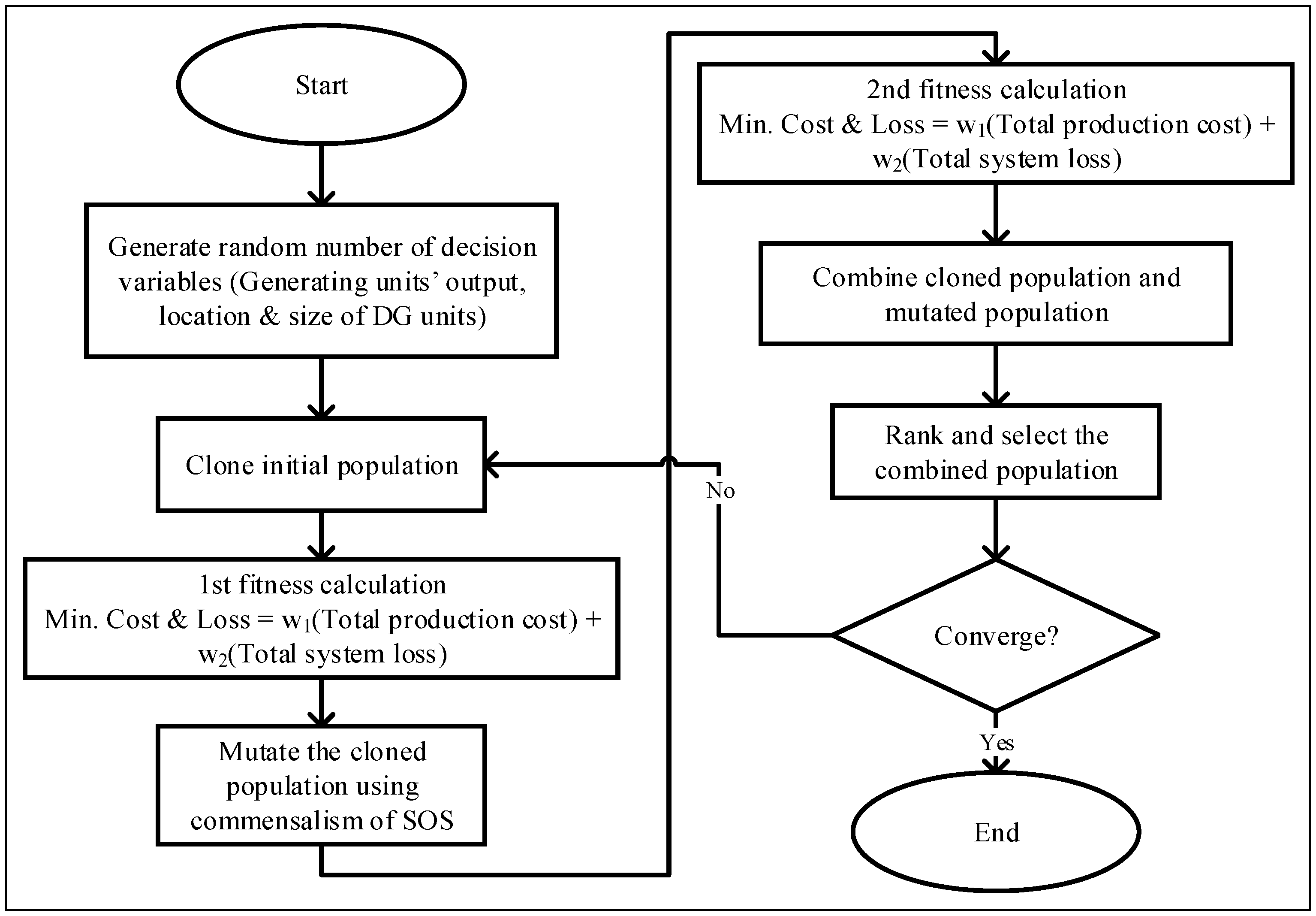
2. Proposed Weighted-Sum Multi-Objective Immune-Commensal-Evolutionary Programming for Total Production Cost and Total System Loss Minimization

In this study, the total production cost and total system loss are optimized simultaneously using the weighted-sum Multi-Objective Immune-Commensal-Evolutionary Programming (MOICEP) technique. The total production is calculated using Equation (1) for the basic ED problems and ED problems with prohibited operating zones, while Equation (2) is used to calculate the total production cost for the ED problems with a valve-point loading effect. The total system loss is calculated using Equation (3).
C t o t a l = i = 1 n C i ( P i ) = i = 1 n a i P i 2 + b i P i + c i
where
  • C i is the production cost of ith generating unit, and
  • P i is the real power output of the ith generating unit.
  • a i , b i and c i are the cost coefficients of the ith generating unit and
  • n is the number of dispatchable generating units:
C t o t a l = i = 1 n C i ( P i ) = i = 1 n a i P i 2 + b i P i + c i + | e i s i n ( f i ( P i m i n P i ) ) |
where e i and f i are the valve-point loading effect coefficients of the ith generating unit.
P l o s s = k = 1 l g k [ V i 2 + V j 2 2 V i V j c o s ( δ i δ j ) ] ,   k { 1 , 2 , , l }
where
  • g k is the conductance of k t h line,
  • V i and δ i are the voltage magnitude and angle of bus i , respectively,
  • V j and δ j are the voltage magnitude and angle of bus j , respectively, and
  • l is the number of lines in the system.
The implementation of this proposed technique is illustrated in Figure 1. The procedure of minimizing the total production costs and total system loss using MOICEP shown in Figure 1 is explained in the following steps.
  • Step 1: Generate decision variable
MOICEP starts with the randomization of the decision variable values based on their constraints. There are three types of decision variables for this problem: real power output of generating units, location of DG units and size of DG units. This randomization is a part of the initialization process of MOICEP. Twenty individuals of each decision variable are stored in the initialization pool that satisfied the constraint violation test. The group of individuals in the pool is called as the initial population.
  • Step 2: Cloning process
Subsequently, the initial population is cloned to increase its size to two hundred. The fitness of this multi-objective is then calculated using Equation (4). The weight coefficients are varied depending on the problem’s desired output. For this study, there were five settings of weight coefficients used to minimize the total production costs and total system loss, which are w 1 = 0.9 , w 2 = 0.1 , w 1 = 0.5 , w 2 = 0.5 , and w 1 = 0.1 , w 2 = 0.9 .
F ( x ) = w 1 f 1 ( x ) + w 2 f 2 ( x )
where
  • F ( x ) is weighted objective function,
  • w 1 is weight coefficient for the first objective function,
  • w 2 is weight coefficient for the second objective function
  • f 1 ( x ) is the first objective function (total production cost minimization) and
  • f 2 ( x ) is the second objective function (total system loss minimization).
  • Step 3: Mutation process
Then, the best two hundred cloned individuals that produce the best value of fitness are mutated using the commensalism equation of the Symbiotic Organisms Search (SOS), as shown in Equation (5). This mutation process is conducted to produce offspring of the mutated population. There are two hundred individual offspring after this process.
X i , n e w = X i + r a n d ( 1 , 1 ) × ( X b e s t X j )
where
  • X i , n e w is the offspring of the ith individual,
  • X i is the parent of the   i th individual,
  • X b e s t is the fittest individual and
  • X j is another individual besides the ith individual.
  • Step 4: Combination process
The cloned population and the mutated populated are then combined to become a large population with the size of four hundred.
  • Step 5: Ranking and selection process
From these four hundred individuals, the twenty best individuals will be selected to undergo the convergence process. However, prior to that, the combined individuals are ranked based on their fitness. Those who give the best value of fitness will be included into the best twenty group; otherwise, they will be excluded from undergoing the next process.
  • Step 6: Convergence test
Subsequently, the best twenty individuals will undergo the convergence process. In this convergence process, a stopping criterion is set to indicate that the algorithm has found the global optima of the multi-objective optimization problem. The stopping criterion used is as shown in Equation (6). If the stopping criterion is not met, the process will proceed to the cloning process and repeat the previous whole steps until the solution converges.
f i t n e s s m a x f i t n e s s m i n 0.0001
where
  • f i t n e s s m a x is the maximum fitness value and
  • f i t n e s s m i n is the minimum fitness value.

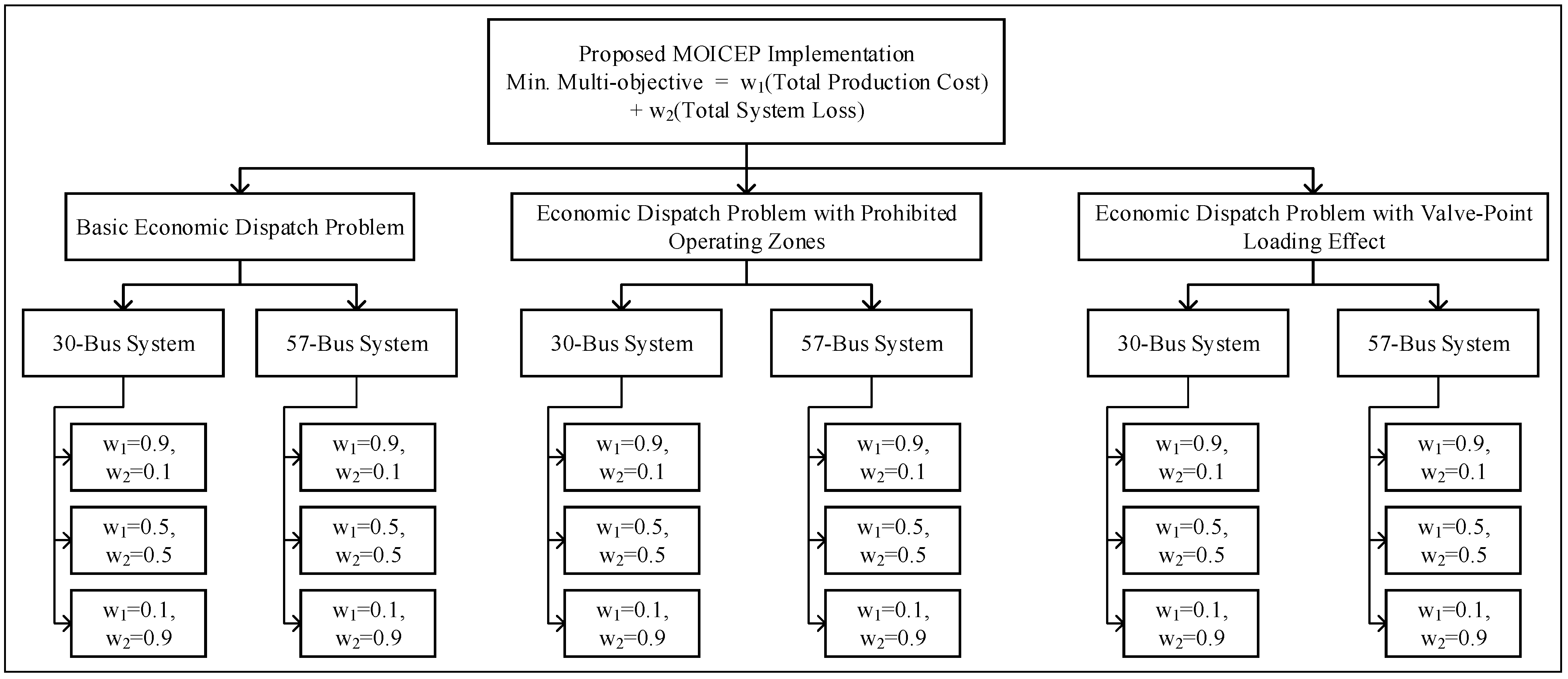
3. Results and Discussion

This section presents the results and discussion on Multi-Objective Immune-Commensal-Evolutionary Programming (MOICEP) for the total production costs and total system loss minimization via integrated Economic Dispatch and Distributed Generation installation (ED-DG). As mentioned previously, the weight coefficients of the objective functions can be varied from 0 to 1.0 between the two objective functions (total production cost minimization and total system loss minimization) to find the trade-off between the two objective functions. The set of weight coefficients for the two fitness functions are as shown in Table 1. The objective functions for this multi-objective problem are the total production cost and total system loss minimization. It can be seen from the table that the summation of w 1 and w 2 is equal to one. If the weight of one of the fitness functions is set to one, then the weight for the other fitness function will be zero. This means that only the objective function with the value of one is optimized, and the other fitness function is not optimized. If the weight value is more than zero, it means that the fitness function is optimized with the amount of the weight. The difference between the fitness and objective functions needs to be understood. Fitness is the equation for the problem formulation, while the objective function is the minimization or the maximization of the fitness function. Let us say, our fitness function f 1 = f 1 ( x ) ; thus, the objective function will be m a x   ( f 1 ( x ) ) or m i n   ( f 1 ( x ) ) .
As suggested by N. A. Rahmat [14], the best settings of the weight coefficients (trade-off) for optimizing the two objective functions were settings 2, 6 and 10, as shown in Table 1. This was because the other settings produced the same nondominated values as settings 2, 6 and 11. Therefore, in this study, the weighted-sum Multi-Objective Immune-Commensal-Evolutionary Programming (MOICEP) technique applied settings 2, 6 and 10 for minimizing the total production costs and total system loss minimization simultaneously.
The overall implementation of the MOICEP is illustrated in Figure 2. The proposed technique has been used to minimize the total production costs and total system loss for three different ED problems. The problems are a basic ED problem, ED problem with prohibited operating zones and ED problem with a valve-point loading effect. Furthermore, for each ED problem, two test systems are used for implementing the MOICEP, which are IEEE 30-Bus RTS and IEEE 57-Bus RTS.

3.1. MOICEP-Based Technique for Basic Economic Dispatch Problem

For this basic ED problem (smooth cost function), Equations (1) and (3) are used to calculate the total production cost and total system loss, respectively. The MOICEP was implemented on the IEEE 30-Bus RTS and IEEE 57-Bus RTS. For each test system, there are five settings of weight coefficients of the two objectives (total production cost minimization and total system loss minimization). The settings are w 1 = 0.9 , w 2 = 0.1 , w 1 = 0.5 , w 2 = 0.5 and w 1 = 0.1 , w 2 = 0.9 . w 1 is the weight coefficient of objective 1 (total production cost minimization), while w 2 is weight coefficient of objective 2 (total system loss minimization).

3.1.1. For w 1 = 0.9 and w 2 = 0.1

The results of the integrated Basic ED and DG installation of the IEEE 30-Bus and 57-Bus RTSs for the second setting of the weight coefficients ( w 1 = 0.9 and w 2 = 0.1 ) are tabulated in Table 2 and Table 3, respectively.
From Table 2, it can be seen that MOICEP continued to give the best solution of the basic ED and DG installation of the IEEE 30-Bus RTS by producing the lowest total production costs and total system loss of 355.91 $/h and 1.44 MW, respectively. The locations of the three DG units found via MOICEP were bus 29, bus 9 and bus 5 with the sizes of 5.00, 50.00 and 100.00 MW, respectively. While the locations and sizes for the three DG units found via MOEP were bus 19 with 4.62 MW, bus 28 with 27.70 MW and bus 5 with 75.81 MW. MOAIS identified bus 19 with 4.62 MW, bus 28 with 27.70 MW and bus 25 with 101.63 MW, respectively. MOEP and MOAIS produced total production costs and total system losses of 463.64 $/h and 2.60 MW and 402.50 $/h and 2.28 MW, respectively. These values were higher than the MOICEP. The proposed MOICEP performed much better than MOEP and MOAIS.
For the results of the IEEE 57-Bus RTS shown in Table 3, similar pattern of results as for the IEEE 30-Bus RTS could be seen. MOICEP maintained producing the lowest total production cost and total system loss of 33285.97 $/h and 9.90 MW, respectively, whereas MOEP and MOAIS found the same total production cost and total system loss of 35,369.69 $/h and 18.95 MW. The optimal location determined by the MOICEP to install the three DG units were bus 25, bus 22 and bus 13 with the sizes of 4.84 MW, 49.99 MW and 150.00 MW, respectively, while MOEP and MOAIS identified bus 33, bus 10 and bus 40 to install the three DG units (Lo1, Lo2 and Lo3) with the sizes of 2.66, 36.55 and 141.03 MW, respectively. MOICEP forced generating unit 8, PG8, to produce the highest power to the system, while generating unit 12, PG12, produced the highest power in MOEP and MOAIS.

3.1.2. For w 1 = 0.5 and w 2 = 0.5

The results value for w 1 was set to 0.5, and w 2 was 0.5 as the third setting. For the third setting of the weight coefficients, the results of the IEEE 30-Bus RTS and IEEE 57-Bus RTS are tabulated in Table 4 and Table 5, respectively.
From Table 4, the MOICEP achieved 402.50 $/h as the total production cost and 1.40 MW for the total system loss. These values were the lowest compared to MOEP (557.01 $/h and 2.25 MW) and MOAIS (429.30 $/h and 2.28 MW). The best total production cost and total system loss in MOICEP were contributed through the placement of DG1, DG2 and DG3 at bus 29, bus 21 and bus 5 with the sizes of 5.00 MW, 31.87 MW and 101.63 MW, respectively. Generating unit 5, PG5, produced the least power in MOICEP, while generating unit 8, PG8, and generating unit 13, PG13, in MOEP and MOAIS, respectively. Apparently, MOICEP consistently outperformed MOEP and MOAIS.
From the results of the IEEE 57-Bus shown in Table 5, it can be seen that MOICEP continued to produce better total production costs and total system loss as compared to MOEP and MOAIS. MOICEP produced 37,513.91 $/h and 9.90 MW, while MOEP and MOAIS produced 38,111.41 $/h and 13.26 MW and 37,752.82 $/h and 14.61 MW, respectively. Bus 35, bus 38 and bus 3 were determined as the optimal locations to install DG1, DG2 and DG3. The corresponding sizes for the three DG units were 3.65 MW, 44.23 MW and 68.97 MW. Generating unit 2, PG2, produced the least power output compared to the other generating units in MOICEP and MOEP, while generating unit 1, PG1, in MOAIS. From the results when w 1 = 0.5 and w 2 = 0.5 , it is observed that the total production cost was slightly expensive, and the total system loss was lower than the previous two settings of weight coefficients.

3.1.3. For w 1 = 0.1 and w 2 = 0.9

The fourth setting was w 1 = 0.1 and w 2 = 0.9 . For this fourth setting of the weight coefficients, the results of integrated Basic ED and DG installation of the IEEE 30-Bus RTS and IEEE 57-Bus RTS are tabulated in Table 6 and Table 7, respectively. From the comparison of the results between the three techniques (MOICEP, MOEP and MOAIS), it was observed that the total production cost produced by MOAIS was the lowest, while the total system loss produced by MOICEP was the lowest. The total production cost in MOAIS was lower than in MOICEP and MOEP, because the total DG size for the three DG units was the highest, worth 133.95 MW compared to MOICEP (121.26 MW) and MOEP (98.08 MW). However, MOICEP still exhibited the lowest total system loss of 1.39 MW as compared to MOEP (2.25 MW) and MOAIS (2.28 MW). Bus 29, bus 21 and bus 5 were the optimal locations to install DG1, DG2 and DG3. The corresponding sizes for the three DG units were 5.00, 29.77 and 86.49 MW. Generating unit 1, PG1, in MOICEP produced the lowest power output, while, in MOEP, generating unit 8, PG8, and, in MOAIS, generating unit 13, PG13, were the ones with the lowest power outputs.
For the results of IEEE 57-Bus RTS shown in Table 7, both the total production cost and total system loss for this setting of weight coefficients ( w 1 = 0.1 and w 2 = 0.9 ) were found to be the lowest in MOICEP, which were 36,159.62 $/h and 6.52 MW as compared to MOEP with 38,111.41 $/h and 13.26 MW and MOAIS with 37,752.82 $/h and 14.61 MW. The optimal locations to install the three DG units identified by MOICEP were bus 25, bus 23 and bus 13 with the corresponding sizes of 4.99, 44.63 and 123.36 MW, respectively. It could be observed that MOICEP forced the DG units to operate near to their maximum capacity. This was the reason why the total production cost reduced significantly as compared to MOEP and MOAIS.

3.2. MOICEP-Based Technique for Economic Dispatch Problem with Prohibited Operating Zones

The proposed MOICEP technique was also used to solve the ED problem with prohibited operating zones. In this study, the same equations of the total production cost (Equation (1)) and total system loss (Equation (3)) in the first ED problem were reutilized. However, there was a difference in the constraint of the operating limits of the generating units. The generating units would only be allowed to operate in the allowable zones to make sure the stability of their operation. The allowable and prohibited zones for the IEEE 30-Bus RTS and IEEE 57-Bus RTS are shown in Table 8 and Table 9, respectively.

3.2.1. For w 1 = 0.9 and w 2 = 0.1

The integrated ED problem with prohibited operating zones and DG installation continued to be solved using MOICEP, MOEP and MOAIS for the second setting of weight coefficients ( w 1 = 0.9 and w 2 = 0.1 ). The results for this setting are shown in Table 10 (IEEE 30-Bus RTS) and Table 11 (IEEE 57-Bus RTS). Similar to the first setting, the solutions produced by MOEP and MOAIS were the same for both systems. From Table 10 of the IEEE 30-Bus RTS, the total production cost and total system loss produced by MOICEP were 380.05 $/h and 1.71 MW, respectively. While MOEP and MOAIS produced a total production cost of 503.05 $/h and total system loss of 3.81 MW. MOICEP significantly outperformed MOEP and MOAIS.
For the DG installation, it was found that bus 29 with 5.00 MW, bus 21 with 50.00 MW and bus 5 with 100.00 MW were the optimal locations and sizes for the three DG units in the IEEE 30-Bus RTS, while, for the IEEE 57-Bus RTS, as shown in Table 11, bus 25, bus 14 and bus 13 were found to be the suitable locations to install the three DG units with the sizes of 3.87, 50.00 and 150.00 MW, respectively, via MOICEP. This resulted in a total production cost and total system loss worth 33,315.31 $/h and 11.29 MW, respectively.
Generating unit 6, PG6, was found to be the least generating unit supplying its real power output to the IEEE 57-Bus RTS in MOICEP, while generating unit 2, PG2, in MOEP and MOAIS. Comparing the total production cost produced in this second setting with the first setting, it can be observed that the total production cost in the second setting was higher for both systems. This was due to the value of w 1 decreasing to 0.1 and the value of w 2 increasing to 0.1 in the second setting.

3.2.2. For w 1 = 0.5 and w 2 = 0.5

Table 12 and Table 13 show the results of the integrated ED problem with the prohibited operating zones and DG installation of the IEEE 30-Bus RTS and IEEE 57-Bus RTS, respectively, with weight coefficients w 1 = 0.5 and w 2 = 0.5 .
Again, MOEP and MOAIS produced the same solution for both systems. As referred to in Table 12, MOICEP produced a total production cost of 492.48 $/h and total system loss of 1.84 MW, while MOEP and MOAIS produced a similar total production cost of 559.24 $/h and a similar total system loss of 3.34 MW. MOICEP managed to save about 66.76 $/h in the total production cost. Besides that, the total system loss found via MOICEP was almost half of the total system loss produced via MOEP and MOAIS.
According to Table 13 for the IEEE 57-Bus RTS, MOICEP managed to produce the lowest total production cost of 35,926.32 $/h and total system loss of 11.83 MW. MOEP and MOAIS produced a similar total production cost of 36,146.27 $/h and a similar total system loss of 12.75 MW. MOICEP identified the optimal locations of DG1, DG2 and DG3 in the IEEE 57-Bus RTS at bus 57, bus 36 and bus 43, respectively. The sizes for the three DG units were 4.52, 44.13 and 101.28 MW. MOEP and MOAIS identified bus 50, bus 33 and bus 10 as the optimal locations to install DG1, DG2 and DG3 with the sizes of 3.62, 23.72 and 120.12 MW, respectively. Generating unit 8, PG8, was found to be the highest generating unit to supply a real power output to the IEEE 57-Bus RTS in MOICEP. In MOEP and MOAIS, generating unit 12, PG12, was the highest contributor of real power output to the system.

3.2.3. For w 1 = 0.1 and w 2 = 0.9

The results of the fourth setting of the weight coefficients ( w 1 = 0.1 and w 2 = 0.9 ) for the IEEE 30-Bus RTS and IEEE 57-Bus RTS are tabulated in Table 14 and Table 15, respectively. As referred to in the two tables, it can be seen that MOEP and MOAIS continued to produce the same solution of the integrated ED problem with prohibited operating zones and DG installation. This could be due to the prohibited operating zones of the generating units that make the searching space of the MOEP and MOAIS algorithms smaller and lead to the same global optima. MOICEP achieved a total production cost of 517.76 $/h and total system loss of 1.49 MW for the IEEE 30-Bus RTS, while, in the IEEE 57-Bus RTS, 35,184.12 $/h and 6.94 MW. As referred to in Table 14, the optimal locations to install DG1, DG2 and DG3 in the IEEE 30-Bus RTS were bus 29, bus 21 and bus 5 with the sizes of 5.00, 27.69 and 85.03 MW, respectively.
On the other hand, in MOEP and MOAIS, the locations and sizes were bus 23 with 3.84 MW, bus 10 with 42.29 MW and bus 27 with 54.73 MW. The six generating units (PG1, PG2, PG5, PG8, PG11 and PG13) in MOICEP produced 13.55, 38.62, 27.96, 34.17, 16.25 and 36.61 MW, respectively. In MOEP and MOAIS, they produced 57.48, 20.05, 42.07, 17.98, 18.35 and 30.00 MW, respectively. Generating unit 1, PG1, in MOICEP produced the lowest real power output compared to the other units. Generating unit 8, PG8, produced the lowest real power output in MOEP and MOAIS.
According to Table 15 of the IEEE 57-Bus RTS, bus 21, bus 26 and bus 13 were found to be the optimal locations to install DG1, DG2 and DG3, respectively. Their sizes were 4.99 MW, 34.73 and 150.00 MW, respectively.
Meanwhile, in MOEP and MOAIS, bus 3, bus 53 and bus 16 were the optimal locations to install DG1, DG2 and DG3 with the sizes of 4.87, 28.54 and 77.88 MW, respectively. It was observed that generating unit 2, PG2, in MOICEP produced a very little real power output of 1.04 MW compared to the other units. The lowest real power output produced by a generating unit in MOEP and MOAIS was 10.46 MW, which was generating unit 2, PG2.

3.3. MOICEP-Based Technique for Economic Dispatch Problem with Valve-Point Loading Effect

The total production cost and total system loss for this type of ED problem were calculated using Equations (2) and (3), respectively. The cost function of this ED was not smooth because of the valve-point loading effect of the generating unit considered in the cost function. The results of the integrated ED problem with a valve-point loading effect and DG installation are observed and discussed in this section.

3.3.1. For w 1 = 0.9 and w 2 = 0.1

Table 16 and Table 17 show the results of the integrated ED problem with a valve-point loading effect and DG installation of the IEEE 30-Bus RTS and 57-Bus RTS with w 1 = 0.9 and w 2 = 0.1 , respectively. It can be seen from Table 16 that MOICEP maintained producing the best solution of an ED with a valve-point loading effect and DG installation for the second setting of the weight coefficients by giving the lowest total production cost of 11,817.81 $/h and the lowest total system loss of 2.04 MW. MOEP and MOAIS produced 13,331.25 $/h and 3.61 MW and 11,627.07 $/h and 13.32 MW, respectively. The best solution from MOICEP was backed by the placement of DG1, DG2 and DG3 at bus 26, bus 5 and bus 9 with the sizes of 5.00, 50.00 and 100.00 MW, respectively. Generating unit 1, PG1, and generating unit 8, PG8, produced the lowest and the highest real power outputs in MOICEP, respectively. The most expensive total production cost was obtained in MOEP, which was 13,331.25 $/h. However, MOAIS produced the highest total system loss of 13.32 MW compared to the other two techniques. It was five times more than the total system loss produced via MOICEP.
As referred to in Table 17 of the IEEE 57-BUS RTS, it can be seen that MOICEP produced the cheapest total production cost of 32,560.84 $/h and total system loss of 9.78 MW compared to MOEP and MOAIS. MOEP and MOAIS produced the same solution, with the total production cost of 35,369.69 $/h and total system loss of 18.95 MW.
MOICEP found bus 26, bus 10 and bus 14 as the optimal locations to install DG1, DG2 and DG3 with the sizes of 5.00, 49.96 and 149.98 MW, respectively. MOEP and MOAIS identified bus 33, bus 10 and bus 40 as the optimal locations to install DG1, DG2 and DG3 with the sizes of 2.66, 36.55 and 141.03 MW, respectively. It was observed that the real power output of the three DG units was higher in MOICEP compared to the real power output in MOEP and MOAIS.

3.3.2. For w 1 = 0.5 and w 2 = 0.5

The third setting of the weight coefficients for solving the integrated ED problem with a valve-point loading effect and DG installation for the IEEE 30-Bus RTS and IEEE 57-Bus RTS are tabulated in Table 18 and Table 19. Referring to Table 18, it can be seen that MOICEP managed to provide a better solution of ED with a valve-point loading effect and DG installation by producing a total production cost of 11,758.98 $/h and total system loss of 1.50 MW compared to MOEP (13,340.00 $/h and 3.31 MW) and MOAIS (13,178.04 $/h and 2.28 MW). This was caused by the placement of DG1, DG2 and DG3 at bus 18, bus 9 and bus 5 with the sizes of 5.00 MW, 50.00 MW and 100.00 MW, respectively. The total DG size was the highest in MOICEP (155.00 MW), while, for MOEP, it was 125.91 MW and, for MOAIS, it was 133.95 MW. Generating unit 1, PG1, produced the lowest real power output of 7.05 MW compared to the other generating units in MOICEP.
The results of the IEEE 57-Bus are shown in Table 19. It can be observed that MOICEP continued to produce a better solution of the integrated ED problem with a valve-point loading effect and DG installation. This was based on the total production cost and total system loss produced, which were the lowest at 33,447.51 $/h and 7.10 MW, respectively. MOEP and MOAIS produced the same results, with a total production cost of 38,013.28 $/h and total system loss worth 13.26 MW.
In MOICEP, bus 25, bus 22 and bus 13 were identified as the best locations to install DG1, DG2 and DG3 with the sizes of 4.97, 42.96 and 150.00 MW, respectively. The generating units 1, 2, 5, 6, 8, 9 and 12 produced real power outputs of 131.64, 36.11, 65.13, 72.78, 273.04, 100.00 and 381.24 MW, respectively.
MOEP and MOAIS identified bus 45, bus 30 and bus 55 as the optimal locations to place DG1, DG2 and DG3 with the sizes of 3.53, 24.77 and 132.47 MW, respectively. The total DG size was higher in MOICEP, which was 197.93 MW compared to MOEP and MOAIS, which was 160.77 MW. As a result, MOICEP achieved a lower total production cost than MOEP and MOAIS.

3.3.3. For w 1 = 0.1 and w 2 = 0.9

The breadth of this study was expanded with the next weight coefficient setting, i.e., w 1 = 0.1 and w 2 = 0.9 . Table 20 and Table 21 show the results of the integrated ED problem with a valve-point loading effect and DG installation of the IEEE 30-Bus RTS and IEEE 57-Bus RTS, respectively.
From Table 20, it can be seen that MOICEP achieved the lowest total system loss of 1.47 MW compared to MOEP (2.34 MW) and MOAIS (2.28 MW). However, the total production cost produced in MOAIS was the lowest compared to MOICEP and MOEP. MOAIS produced a total production cost of 13,178.04 $/h, while MOICEP and MOEP produced 13,472.72 $/h and 15,179.41 $/h, respectively. The highest total production cost was found in MOEP. The optimal locations and sizes found via MOICEP for DG1, DG2 and DG3 were bus 29 with 5.00 MW, bus 22 with 28.71 MW and bus 5 with 86.75 MW. It was observed that, to make sure the total system loss was the lowest, MOICEP avoided the three DG units operating near their maximum capacity.
A similar observation was experienced by the IEEE 57-Bus RTS, as shown in Table 21; the total system loss produced via MOICEP was the lowest. However, the total production cost was the highest compared to MOEP and MOAIS. MOICEP produced a total production cost of 38,352.96 $/h and total system loss of 8.35 MW. MOEP and MOAIS produced the same results, with a total production cost of 38,013.28 $/h and total system loss of 13.26 MW. The optimal locations to install DG1, DG2 and DG3 in the IEEE 57-Bus RTS via MOICEP were bus 29, bus 22 and bus 13 with the sizes of 1.03, 44.02 and 59.53 MW, respectively. The total system loss produced via MOICEP was 37.03% lower than the total system loss produced via MOEP and MOAIS. However, in terms of the total production cost, MOICEP did not force the three DG units to operate near their maximum capacity. This resulted in a high total production cost produced via MOICEP. It must be kept in mind that the weight coefficients also play an important role that leads to the results. As the value of w 1 decreases and the value of w 2 increases, the algorithm tends to focus on optimizing objective function 2 (total system loss), as expected.

4. Conclusions

The new Multi-Objective Immune-Commensal-Evolutionary Programming (MOICEP) technique for the total production cost and total system loss minimization via integrated Economic Dispatch and Distributed Generation installation (ED-DG) was presented in this paper. It was employed for the total production cost and total system loss minimization in an integrated weighted-sum multi-objective optimization technique for solving the ED problem with DG installation consideration. This scheme is uniquely termed as Economic Dispatch and Distributed Generation installation (ED-DG). The proposed weighted-sum multi-objective function that integrated both the total production cost and total system loss was highlighted in this study. The introduction of weight coefficients in the proposed fitness exhibited convincing results in addressing both components. The weight coefficients were varied between 0.1 and 0.9 to find the optimal solution that satisfied both the total production cost and total system loss. From the variations, it could be seen that, as the value of w 1 was greater than w 2 , the solution produced favored total production cost minimization, while, if the value of w 2 was greater than w 1 , the solution favored total system loss minimization. GSOs can decide which solution is the best for their system requirements and their desired output. The proposed MOICEP technique managed to achieve better results over benchmarked techniques, i.e., MOEP and MOAIS, for the minimization of the total production costs and total system loss for three types of ED problems (basic ED, ED problem with prohibited operating zones and an ED problem with a valve-point loading effect). This phenomenon highlights the superiority of MOICEP over MOEP and MOAIS. This phenomenon has been identified as cutting edge in ED problems as the original independent scheme, i.e., ED and DG installation. The proposed multi-objective technique could be feasible for solving other optimization problems with considerable fine-tuning. It is also beneficial for power system utilities in solving their ED problems. It can also be concluded that, while optimizing the two objectives, total production cost and total system loss, the integrated Economic Dispatch and Distributed Generation installation ED-DG problems solved using the proposed MOICEP technique simultaneously solved two power system problems, ED and DG installation, which have been previously solved separately by many researchers. The two objectives are inextricably linked to the two problems.
The number of objectives for the multi-objective ED problems can be increased in the future. This can be done by adding more objectives like voltage stability improvement, emission minimization and DG installation cost minimization into the integrated ED-DG problems.

Author Contributions

All the authors listed conceived and designed the project. Conceptualization, M.H.M. and I.M.; acquired the funding, M.H.M.; methodology, M.H.M., I.M. and M.M.O.; validation, M.H.M. and I.M.; analysis, M.H.M. and M.M.O.; writing—original draft preparation, M.H.M. and I.M. and writing—review and editing, M.M.O. All authors have read and agreed to the published version of the manuscript.

Funding

This research was funded by the Ministry of Higher Education Malaysia (MOHE), grant number FRGS/1/2020/TK0/UNITEN/03/4.

Institutional Review Board Statement

Not applicable.

Informed Consent Statement

Not applicable.

Conflicts of Interest

The authors declare no conflict of interest.

References

  1. Mehigan, L.; Deane, J.P.; Gallachóir, B.P.Ó.; Bertsch, V. A review of the role of distributed generation (DG) in future electricity systems. Energy 2018, 163, 822–836. [Google Scholar] [CrossRef]
  2. Zhan, J.; Wu, Q.H.; Guo, C.; Zhou, X. Economic Dispatch With Non-Smooth Objectives—Part I: Local Minimum Analysis. IEEE Trans. Power Syst. 2015, 30, 710–721. [Google Scholar] [CrossRef]
  3. Thenmalar, K.; Anujak, S.; Ramesh, S. Multi-Objective economic emission load dispatch solution using wolf’s method in various generation plants with wind power penetration. In Proceedings of the 2014 International Conference on Electronics and Communication Systems, ICECS 2014, Coimbatore, Tamilnadu, 13–14 February 2014; pp. 1–13. [Google Scholar]
  4. Jakob, W.; Blume, C. Pareto optimization or cascaded weighted sum: A comparison of concepts. Algorithms 2014, 7, 166–185. [Google Scholar] [CrossRef] [Green Version]
  5. Marler, R.T.; Arora, J.S. The weighted sum method for multi-objective optimization: New insights. Struct. Multidiscip. Optim. 2010, 41, 853–862. [Google Scholar] [CrossRef]
  6. Musau, M. Multi Area Multi Objective Dynamic Economic Dispatch with Renewable Energy and Emissions. In Proceedings of the 2016 IEEE International Energy Conference (ENERGYCON), Leuven, Belgium, 4–8 April 2016; pp. 112–117. [Google Scholar]
  7. Roy, N.; Ghosh, A.; Sanyal, K. Normal Boundary Intersection based multi-objective Harmony Search algorithm for environmental Economic Load Dispatch problem. In Proceedings of the 2016 IEEE 6th International Conference on Power Systems, ICPS 2016, New Delhi, India, 4–6 March 2016; pp. 1–6. [Google Scholar]
  8. Mohanty, P.S. Multi-objective economic emission load dispatch with nonlinear fuel cost and noninferior emission level functions for IEEE-118 bus system. In Proceedings of the 2nd International Conference on Electronics and Communication Systems (ICECS), Coimbatore, India, 26–27 February 2015; pp. 1371–1376. [Google Scholar]
  9. Mao, M.; Ji, M.; Dong, W.; Chang, L. Multi-objective economic dispatch model for a microgrid considering reliability. In Proceedings of the 2nd International Symposium on Power Electronics for Distributed Generation Systems, PEDG 2010, Hefei, China, 16–18 June 2010; pp. 993–998. [Google Scholar]
  10. Man-Im, A.; Ongsakul, W.; Singh, J.G.; Boonchuay, C. Multi-objective economic dispatch considering wind generation uncertainty using non-dominated sorting particle swarm optimization. In Proceedings of the 2014 International Conference and Utility Exhibition on Green Energy for Sustainable Development, ICUE 2014, Pattaya City, Thailand, 19–21 March 2014; pp. 19–21. [Google Scholar]
  11. Bilil, H.; Ellaia, R.; Maaroufi, M. A New Multi-objective Particle Swarm Optimization for Economic Environmental Dispatch. In Proceedings of the 2012 IEEE International Conference on Complex Systems (ICCS), Agadir, Morocco, 5–6 November 2012; Volume 3, pp. 1–6. [Google Scholar]
  12. Shen, X.; Zou, D.; Duan, N.; Zhang, Q. An efficient fitness-based differential evolution algorithm and a constraint handling technique for dynamic economic emission dispatch. Energy 2019, 186, 1–28. [Google Scholar] [CrossRef]
  13. Yuan, G.; Yang, W. Study on optimization of economic dispatching of electric power system based on Hybrid Intelligent Algorithms (PSO and AFSA). Energy 2019, 183, 926–935. [Google Scholar] [CrossRef]
  14. Rahmat, N.A. Computational Intelligence Based Technique for Solving Economic Dispatch Problem. Ph.D. Thesis, Universiti Teknologi MARA, Shah Alam, Malaysia, 2016. [Google Scholar]
Figure 1. Overall MOICEP processes for the total production costs and total system loss minimization.
Energies 14 07733 g001
Figure 2. Overall implementation of the MOICEP for total production cost and total system loss minimization.
Energies 14 07733 g002
Table 1. Weight coefficients values for two objective functions (total production cost and total system loss).
SettingWeight CoefficientsFitness Function
w 1 w 2 Total Production CostTotal System Loss
110
20.90.1
30.80.2
40.70.3
50.60.4
60.50.5
70.40.6
80.30.7
90.20.8
100.10.9
1101.0
Table 2. Results of the integrated basic ED and DG installation of the IEEE 30-Bus RTS ( w 1 = 0.9 and w 2 = 0.1 ).
Optimization TechniqueMOICEPMOEPMOAIS
Locations of DGs (Bus no.)Lo1291919
Lo292828
Lo35525
Sizes of DGs (MW)DG15.004.624.62
DG250.0027.7027.70
DG3100.0075.81101.63
Generating Unit Output (MW)PG116.4258.4832.36
PG220.0048.6648.66
PG515.0023.3223.32
PG826.2116.8716.87
PG1123.2617.1917.19
PG1328.9513.3313.33
Total Production Cost ($/h)355.91463.64402.50
Total System Loss (MW)1.442.602.28
Table 3. Results of the integrated basic ED and DG installation of the IEEE 57-Bus RTS ( w 1 = 0.9 and w 2 = 0.1 ).
Optimization TechniqueMOICEPMOEPMOAIS
Locations of DGs (Bus no.)Lo1253333
Lo2221010
Lo3134040
Sizes of DGs (MW)DG14.842.662.66
DG249.9936.5536.55
DG3150.00141.03141.03
Generating Unit Output (MW)PG1137.42191.80191.80
PG247.836.686.68
PG522.5758.4558.45
PG671.5968.6868.68
PG8381.87323.93323.93
PG939.4393.0493.04
PG12355.16346.93346.93
Total Production Cost ($/h)33,285.9735,369.6935,369.69
Total System Loss (MW)9.9018.9518.95
Table 4. Results of the integrated basic ED and DG installation of the IEEE 30-Bus RTS ( w 1 = 0.5 and w 2 = 0.5 ).
Optimization TechniqueMOICEPMOEPMOAIS
Locations of DGs (Bus no.)Lo1292719
Lo221728
Lo35525
Sizes of DGs (MW)DG15.004.064.62
DG231.8733.3327.70
DG3101.6360.6994.86
Generating Unit Output (MW)PG118.5421.7532.36
PG224.5160.9548.66
PG515.0038.8223.32
PG835.0015.1316.87
PG1130.0026.7317.19
PG1330.0024.1813.33
Total Production Cost ($/h)402.50557.01429.30
Total System Loss (MW)1.402.252.28
Table 5. Results of the integrated basic ED and DG installation of the IEEE 57-Bus RTS ( w 1 = 0.5 and w 2 = 0.5 ).
Optimization TechniqueMOICEPMOEPMOAIS
Locations of DGs (Bus no.)Lo1354534
Lo2383023
Lo335511
Sizes of DGs (MW)DG13.653.533.44
DG244.2324.7740.05
DG368.97132.4792.34
Generating Unit Output (MW)PG1206.60237.1024.14
PG216.2425.0153.09
PG534.87120.5291.62
PG652.0447.1340.76
PG8351.68278.28450.99
PG981.8260.0471.83
PG12400.55335.20397.14
Total Production Cost ($/h)37,513.9138,111.4137,752.82
Total System Loss (MW)9.9013.2614.61
Table 6. Results of the integrated basic ED and DG installation of the IEEE 30-Bus RTS ( w 1 = 0.1 and w 2 = 0.9 ).
Optimization TechniqueMOICEPMOEPMOAIS
Locations of DGs (Bus no.)Lo1292719
Lo221728
Lo35525
Sizes of DGs (MW)DG15.004.064.62
DG229.7733.3327.70
DG386.4960.69101.63
Generating Unit Output (MW)PG118.6521.7532.36
PG227.9160.9548.66
PG522.0138.8223.32
PG834.9615.1316.87
PG1130.0026.7317.19
PG1330.0024.1813.33
Total Production Cost ($/h)461.64557.01402.50
Total System Loss (MW)1.392.252.28
Table 7. Results of the integrated basic ED and DG installation of the IEEE 57-Bus RTS ( w 1 = 0.1 and w 2 = 0.9 ).
Optimization TechniqueMOICEPMOEPMOAIS
Locations of DGs (Bus no.)Lo1254534
Lo2233023
Lo3135511
Sizes of DGs (MW)DG14.993.533.44
DG244.6324.7740.05
DG3123.36132.4792.34
Generating Unit Output (MW)PG1125.84237.1024.14
PG226.3725.0153.09
PG587.41120.5291.62
PG695.9647.1340.76
PG8238.78278.28450.99
PG9100.0060.0471.83
PG12409.98335.20397.14
Total Production Cost ($/h)36,159.6238,111.4137,752.82
Total System Loss (MW)6.5213.2614.61
Table 8. Cost coefficients and generating unit limits for the ED problem with the prohibited operating zones (IEEE 30-Bus RTS).
Gen. Unit P m i n P m a x Prohibited ZonesCost Coefficients
Zone 1Zone 2 a i b i c i
15020055–6680–1200.003752.000
2208021–2445–550.017501.750
5155030–36-0.062501.000
8103525–30-0.008343.250
11103025–28-0.025003.000
13103024–30-0.025003.000
Table 9. Cost coefficients and generating unit limits for the ED problem with the prohibited operating zones (IEEE 57-Bus RTS).
Gen. Unit P m i n P m a x Prohibited ZonesCost Coefficients
Zone 1Zone 2 a i b i c i
10575.8810–50480–5200.0775795200
201005–1075–800.0100000400
3014010–25100–1100.2500000200
601005–10-0.0100000400
8055010–30-0.0222222200
901005–10-0.0100000400
12041010–35-0.0322581200
Table 10. Results of the integrated ED problem with prohibited operating zones and DG installation of the IEEE 30-Bus RTS ( w 1 = 0.9 and w 2 = 0.1 ).
Optimization TechniqueMOICEPMOEPMOAIS
Locations of DGs (Bus no.)Lo1292424
Lo2211515
Lo352222
Sizes of DGs (MW)DG15.004.034.03
DG250.0049.6049.60
DG3100.0068.2768.27
Generating Unit Output (MW)PG112.2619.4819.48
PG226.7044.9644.96
PG527.4339.5439.54
PG834.2532.7632.76
PG1110.2715.2515.25
PG1319.2013.3313.33
Total Production Cost ($/h)380.05503.05503.05
Total System Loss (MW)1.713.813.81
Table 11. Results of the integrated ED problem with prohibited operating zones and DG installation of the IEEE 57-Bus RTS ( w 1 = 0.9 and w 2 = 0.1 ).
Optimization TechniqueMOICEPMOEPMOAIS
Locations of DGs (Bus no.)Lo1255050
Lo2143333
Lo3131010
Sizes of DGs (MW)DG13.873.623.62
DG250.0023.7223.72
DG3150.00120.12120.12
Generating Unit Output (MW)PG1121.07201.79201.79
PG296.270.770.77
PG543.9253.6853.68
PG634.1441.7541.75
PG8379.12377.72377.72
PG941.1258.9058.90
PG12342.59381.48381.48
Total Production Cost ($/h)33,315.3136,146.2736,146.27
Total System Loss (MW)11.2912.7512.75
Table 12. Results of the integrated ED problem with prohibited operating zones and DG installation of the IEEE 30-Bus RTS ( w 1 = 0.5 and w 2 = 0.5 ).
Optimization TechniqueMOICEPMOEPMOAIS
Locations of DGs (Bus no.)Lo1292323
Lo251010
Lo392727
Sizes of DGs (MW)DG15.003.843.84
DG245.5742.2942.29
DG381.1854.7354.73
Generating Unit Output (MW)PG13.9957.4857.48
PG253.2220.0520.05
PG541.5142.0742.07
PG817.0617.9817.98
PG1110.1418.3518.35
PG1327.5630.0030.00
Total Production Cost ($/h)492.48559.24559.24
Total System Loss (MW)1.843.343.34
Table 13. Results of the integrated ED problem with prohibited operating zones and DG installation of the IEEE 57-Bus RTS ( w 1 = 0.5 and w 2 = 0.5 ).
Optimization TechniqueMOICEPMOEPMOAIS
Locations of DGs (Bus no.)Lo1575050
Lo2363333
Lo3431010
Sizes of DGs (MW)DG14.523.623.62
DG244.1323.7223.72
DG3101.28120.12120.12
Generating unit output (MW)PG1182.78201.79201.79
PG257.290.770.77
PG568.0353.6853.68
PG673.4741.7541.75
PG8363.59377.72377.72
PG929.9158.9058.90
PG12337.61381.48381.48
Total Production Cost ($/h)35,926.3236,146.2736,146.27
Total System Loss (MW)11.8312.7512.75
Table 14. Results of the integrated ED problem with prohibited operating zones and DG installation of the IEEE 30-Bus RTS ( w 1 = 0.1 and w 2 = 0.9 ).
Optimization TechniqueMOICEPMOEPMOAIS
Locations of DGs (Bus no.)Lo1292323
Lo2211010
Lo352727
Sizes of DGs (MW)DG15.003.843.84
DG227.6942.2942.29
DG385.0354.7354.73
Generating Unit Output (MW)PG113.5557.4857.48
PG238.6220.0520.05
PG527.9642.0742.07
PG834.1717.9817.98
PG1116.2518.3518.35
PG1336.6130.0030.00
Total Production Cost ($/h)517.76559.24559.24
Total System Loss (MW)1.493.343.34
Table 15. Results of the integrated ED problem with prohibited operating zones and DG installation of the IEEE 57-Bus RTS ( w 1 = 0.1 and w 2 = 0.9 ).
Optimization TechniqueMOICEPMOEPMOAIS
Locations of DGs (Bus no.)Lo12133
Lo2265353
Lo3131616
Sizes of DGs (MW)DG14.994.874.87
DG234.7328.5428.54
DG3150.0077.8877.88
Generating Unit Output (MW)PG1148.50175.15175.15
PG21.0410.4610.46
PG581.0893.1493.14
PG676.8683.3483.34
PG8254.90319.71319.71
PG999.8265.8665.86
PG12405.81402.63402.63
Total Production Cost ($/h)35,184.1238,362.2838,362.28
Total System Loss (MW)6.9410.8010.80
Table 16. Results of the integrated ED problem with a valve-point loading effect and DG installation of the IEEE 30-Bus RTS ( w 1 = 0.9 and w 2 = 0.1 ).
Optimization TechniqueMOICEPMOEPMOAIS
Locations of DGs (Bus no.)Lo1262529
Lo25274
Lo39718
Sizes of DGs (MW)DG15.001.062.50
DG250.0035.9839.45
DG3100.0093.411.30
Generating Unit Output (MW)PG18.393.7513.23
PG220.0051.7822.77
PG522.2931.2618.40
PG834.4633.5230.59
PG1115.3011.0023.90
PG1330.0025.2316.34
Total Production Cost ($/h)11,817.8113,331.2511,627.07
Total System Loss (MW)2.043.6113.32
Table 17. Results of the integrated ED problem with a valve-point loading effect and DG installation of the IEEE 57-Bus RTS ( w 1 = 0.9 and w 2 = 0.1 ).
Optimization TechniqueMOICEPMOEPMOAIS
Locations of DGs (Bus no.)Lo1263333
Lo2101010
Lo3144040
Sizes of DGs (MW)DG15.002.662.66
DG249.9636.5536.55
DG3149.98141.03141.03
Generating Unit Output (MW)PG1132.46191.82191.82
PG243.986.686.68
PG549.4858.4458.44
PG672.0268.6768.67
PG8327.03323.93323.93
PG973.7893.0493.04
PG12356.90346.92346.92
Total Production Cost ($/h)32,560.8435,369.6935,369.69
Total System Loss (MW)9.7818.9518.95
Table 18. Results of the integrated ED problem with a valve-point loading effect and DG installation of the IEEE 30-Bus RTS ( w 1 = 0.5 and w 2 = 0.5 ).
Optimization TechniqueMOICEPMOEPMOAIS
Locations of DGs (Bus no.)Lo1181619
Lo291928
Lo3595
Sizes of DGs (MW)DG15.003.354.62
DG250.0043.0527.70
DG3100.0079.51101.63
Generating Unit Output (MW)PG17.0512.7732.36
PG220.0039.0548.66
PG515.0046.0423.32
PG834.6526.3016.87
PG1124.7813.0117.18
PG1328.4223.6313.33
Total Production Cost ($/h)11,758.9813,340.0013,178.04
Total System Loss (MW)1.503.312.28
Table 19. Results of the integrated ED problem with a valve-point loading effect and DG installation of the IEEE 57-Bus RTS ( w 1 = 0.5 and w 2 = 0.5 ).
Optimization TechniqueMOICEPMOEPMOAIS
Locations of DGs (Bus no.)Lo1254545
Lo2223030
Lo3135555
Sizes of DGs (MW)DG14.973.533.53
DG242.9624.7724.77
DG3150.00132.47132.47
Generating Unit Output (MW)PG1131.64237.10237.10
PG236.1125.0125.01
PG565.13120.52120.52
PG672.7847.1347.13
PG8273.04278.28278.28
PG9100.0060.0460.04
PG12381.24335.20335.20
Total Production Cost ($/h)33,447.5138,013.2838,013.28
Total System Loss (MW)7.1013.2613.26
Table 20. Results of the integrated ED problem with a valve-point loading effect and DG installation of the IEEE 30-Bus RTS ( w 1 = 0.1 and w 2 = 0.9 ).
Optimization TechniqueMOICEPMOEPMOAIS
Locations of DGs (Bus no.)Lo1292719
Lo222428
Lo3555
Sizes of DGs (MW)DG15.003.124.62
DG228.7135.2027.70
DG386.7550.38101.63
Generating Unit Output (MW)PG112.5226.0332.36
PG241.1260.7348.66
PG520.4638.7823.32
PG835.0033.3716.87
PG1129.1817.6717.18
PG1326.1220.3913.33
Total Production Cost ($/h)13,472.7215,179.4113,178.04
Total System Loss (MW)1.472.342.28
Table 21. Results of the integrated ED problem with a valve-point loading effect and DG installation of the IEEE 57-Bus RTS ( w 1 = 0.1 and w 2 = 0.9 ).
Optimization TechniqueMOICEPMOEPMOAIS
Locations of DGs (Bus no.)Lo1294545
Lo2223030
Lo3135555
Sizes of DGs (MW)DG11.033.533.53
DG244.0224.7724.77
DG359.53132.47132.47
Generating Unit Output (MW)PG1143.43237.10237.10
PG254.9625.0125.01
PG584.08120.52120.52
PG679.6047.1347.13
PG8309.65278.28278.28
PG985.5760.0460.04
PG12397.27335.20335.20
Total Production Cost ($/h)38,352.9638,013.2838,013.28
Total System Loss (MW)8.3513.2613.26
Publisher’s Note: MDPI stays neutral with regard to jurisdictional claims in published maps and institutional affiliations.

