Abstract
The analytical solutions of complex dynamic PRO systems pose challenges to ensuring that maximum power can be harvested in stable, rapid, and efficient ways in response to varying operational environments. In this paper, a boosted particle swarm optimization (BPSO) method with enhanced essential coefficients is proposed to enhance the exploration and exploitation stages in the optimization process. Moreover, several state-of-the-art techniques are utilized to evaluate the proposed BPSO of scaled-up PRO systems. The competitive results revealed that the proposed method improves power density by up to 88.9% in comparison with other algorithms, proving its ability to provide superior performance with complex and computationally intensive derivative problems. The analysis and comparison of the popular and recent metaheuristic methods in this study could provide a reference for the targeted selection method for different applications.
1. Introduction
The hydrological cycle of nature provides significant renewable energy sources (RES) through the salinity gradient. Chemical potential energy is increasingly considered a promising RES that can resolve the problems of carbon emissions, air pollution, global energy shortages, and the high price of fossil fuels. Pressure retarded osmosis (PRO) is therefore developed and investigated as a popular clean energy production method using the natural salinity gradient technology to mitigate such phenomena [1,2,3,4]. This sustainable power can be yielded by mixing solutions of two different salt concentrations, such as seawater mixed with fresh river water. The potential extractable energy is estimated to be a huge amount, equivalent to 1.724–3.158 TW [5], and hence it attracts a lot of academic and commercial interest. Among PRO, capacitance mixing (CapMix), reverse electrodialysis (RED), hydrogel swelling, battery mixing, and other salinity gradient power generation technologies, PRO has higher power density and efficiency [6,7]. Therefore, it has been most widely studied.
At present, the energy efficiency of PRO systems is low. At the stage of implementation, economically, a software upgrade that replaces MPPT with an advanced and efficient algorithm presents a negligible cost increase. The first MPPT research for PRO systems was conducted in 2015, considering dynamic changes, including incremental mass resistance (IMR) as well as perturbation and observation (P&O) methods [8]. Both algorithms have to find a balance between oscillations and the response time, resulting in greater power loss [9]. Studies have shown that the operational environment depends on specific circumstances, materials, and other constraints [10]. However, modelling and design efforts for PRO systems cannot adapt to changing environmental conditions, and it is difficult to make real-time adjustments under operating constraints. Therefore, real-time control of PRO power system-based MPPT has been investigated most recently [9,11]. The research of the MPPT control methods is of great significance for improving the performance of the PRO system under varying operational conditions. It can be implemented not only on the stand-alone PRO system, but also on the hybrid PRO system and other RES systems.
There are currently two main criteria utilized to rate the efficiency of MPPT algorithms, namely the extractable power density and the convergence time. The higher the tracking speed, the higher the extracted power and the smaller the output power loss, and vice versa. A shorter tracking time results in higher oscillations. The optimization algorithm has unique advantages in improving methods and systems in the engineering field, especially for complex and computationally intensive derivative problems in the unknown search space, which are capable of avoiding the local optima entrapments and steady-state oscillation of the classic MPPT algorithm. A method for the real-time control of PRO systems using feedback control have been proposed [9]. However, the actual complex and dynamic operating environment has not been taken into consideration. Considering the actual detrimental effects, the whale optimization algorithm (WOA)-based MPPT control algorithm of the PRO system was studied under fluctuating salinity conditions, and it showed encouraging performance [11]. However, the temperature effect was not considered.
The motivation and significance of this work are threefold. First, there is limited published research work on the maximum power density tracking of dynamic PRO models [8,9,11]. The analytical solutions of complex dynamic systems pose challenges to MPPT strategies to ensure that maximum power can be harvested in stable, rapid, and efficient ways in response to varying operational environments. Inspired by the dispersion and self-organizing behaviors of animal herds in nature, metaheuristic technology has been extensively studied and explored in recent years. Not only do such herds interestingly show the excellence of nature, but they have also proven to be efficient in solving real-world engineering problems. Another motivation is that, according to the no-free-lunch (NFL) theory, no specific optimization method can solve all optimization issues [12]. Thus, if the performance of algorithm X in problem A is better than that of algorithm Y, there must be a set of problem B in which algorithm Y is more efficient than algorithm X. In other words, the best conditions and solutions are case-specific. This well-known theory has inspired an endless stream of researchers that have utilized state-of-the-art optimization algorithms in various groups of issues, as in this study. Third, the proposed method can also be applied to other systems, especially renewable energy systems, such as photovoltaic systems, wind turbine systems, and hybrid renewable systems. This has, therefore, motivated the research and application of metaheuristic-based maximum energy extraction methods in PRO design optimization.
2. Materials and Methods
2.1. Particle Swarm Optimization
A flow chart of the classic PSO-based MPPT technique is illustrated in Figure 1. The particle swarm optimization can be mathematically expressed by updating the position and velocity of the searching agency using the following equations [13].
where is the current iteration and and denote the velocity and position of the th particle, where the position indicates the best-obtained solution in the problem. is an inertia weight parameter equal to 1, and and are constants equal to 1.5 and 2, respectively. and represent the normalized random values in the interval (0, 1), donates the best position found in the ith iteration, and depicts the best acquired global position.
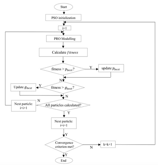
Figure 1.
Flow chart of the PSO-based maximum energy extraction algorithm for the PRO system.
2.2. Boosted Particle Swarm Optimization
Detailed comparisons are listed in Table 1, including the key vectors and essential coefficients in the process of the metaheuristic algorithms. In the essential coefficients of Table 1, the current solution and global optimal position are expressed in the mathematical models as and , respectively. The population position is adopted in the formulations in terms of the average position of the current population, namely and the distance from each particle in the population , respectively.

Table 1.
Detailed comparative analysis concerning the key vectors and essential coefficients in the metaheuristic algorithms.
Among metaheuristic algorithms, the difference between the PSO and some other well-regarded swarm-intelligence-based techniques is twofold. Take HGSO for instance, first, there are two critical vectors in the PSO, namely the velocity and position vectors of each particle. In the HGSO process, only one coefficient position is considered. Second, in the PSO algorithm, the next location of the particle is updated regarding three essential coefficients, namely the current optimal solution, global optimal solution, and current solution. In the HGSO technique, the next step of the searching particle is formulated in consideration of the current solution, optimal global solution, worst solution, and the obtained solution using the population. Compared with the PSO, the HGSO method involves the solutions obtained by the population, thus including more communication between intelligent swarms. This is also another reason why the HGSO is capable of performing better under rapid fluctuation profiles.
Furthermore, a comparison and performance analysis of these proposed metaheuristic-based MPPT strategies is performed, as shown in Table 2. Based on the above analysis, the PSO can be boosted to combine the merits of other strategies considering the population solution and worst solution for better performance.
Table 2.
Detailed comparative analysis of PSO and BPSO.
In the BPSO, the worst agent is replaced with a random solution within the boundaries of the problem with the purpose of enhancing the exploration phase, which is formulated as
where and denote the dimension and the upper and lower boundaries of the system, respectively. The velocity of the particle is updated considering the population location to improve the exploitation process as follows:
where donates the mean best solution in the iteration. The position of the ith particle is calculated as
The process of the proposed BPSO strategy is shown in Figure 2.
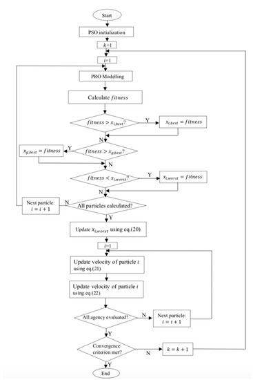
Figure 2.
Flow chart of the BPSO-based maximum energy extraction algorithm for the PRO system.
3. Formulation of the Optimization Problem in the PRO System
3.1. Pressure Retarded Osmosis Model
The proposed method is utilized to solve the MPPT problem in PRO systems, and the performance is validated by simulation. The first PRO model was promoted in 1975 by Loeb [1]. Then, PRO models were developed considering finite element approaches employed to describe axial variations in concentration [3], different membrane types [8], detrimental phenomena, including ICP, ECP, and RSF [10]. The mathematical model for tracking the maximum power density is described and demonstrated above, so here is a brief review [3,8,9,10,14].
The osmotic pressure difference drives the permeate throughout the membrane and applies hydraulic pressure ΔP on the opposite side, namely ‘pressure retarded’. In an ideal PRO system, permeation can be expressed as the water flux , and it is defined as [4]
where denotes the membrane permeability. The osmotic pressure difference between two solutions is represented based on Van’t Hoff’s law as
where is the Van’t Hoff factor, and and denote the draw solution and feed solution concentrations, respectively. The power density is formulated as [10]
The mass transfer functions can be expressed as Equations (4) and (5), which represent a one-dimensional model derived from the unsteady convection-diffusion equation.
where and denote the draw and feed flow rates. Detailly, considering the discharge process of the PRO system in regard to the RSF detrimental effect, the mass flow rates of the permeating solution , and the reverse solute are modelled as
In which and are the density of the permeate and the draw solution, and is the membrane area. In consideration of the limitation of RSF, the concentrations on the draw side and feed side are formulated from the mass transfer equations as [6]
The flow rates of the draw solution and feed solution and are described as
In which is the permeated solution flow rate. and are the initial draw flow rate and feed flow rate, respectively. In fact, due to three inevitable detrimental phenomena, namely ECP, ICP, and RSF, the water flux is lower. The active layer dilutes the solute near its surface and reduces the effect of osmotic pressure on the draw side of the PRO membrane, and the dilutive ECP occurs. The effect of ECP declines the solute concentration from the draw solution to the active layer surface, while the effect of ICP reduces the concentration of feed solution to the active support interface. The effect of driving force across the membrane and water flux is thereby decreased [7]. Moreover, a certain amount of salt permeates through the membrane during osmotic operation, affecting the concentration gradient and the extractable power density [4].
Considering ECP, ICP, and RSF, by solving the mass transfer equations, the water flux and salt flux can be determined as [8,15]
where denote all the membrane parameters, including the salt permeability factors, membrane structural factor, and solute diffusion factor, respectively. and denote the osmotic pressure on the draw and feed sides, respectively. depicts the solute resistivity of the porous membrane support. The water flux model is based on the solution-diffusion model that assumes the transport occurs only by diffusion across membranes. Finally, the water flux across the PRO membrane can be influenced significantly by the mass transfer characteristics. The volume of the final total permeating water is expressed as [4]
Assuming the reversibility, the available extracted energy in a constant-pressure PRO plant can be calculated as the product of the permeate volume and applied energy [7]. The power density varies along the tube, so the extractable energy is utilized to quantify the energy conversion speed, as in [7]
The detailed mathematical model can be found in [11]. It can be observed from the model that the maximum power density and characteristic curves rapidly change with the variations in the operation and salinity conditions. Thus, it is significant to accurately and efficiently track MPPs during osmotic processes.
3.2. Optimization Performance Index
To objectively test the proposed algorithm for the MPPT problem in the PRO system, the following mathematical performance measures are employed.
(1) The average fitness index (AFI) is applied as a significant factor to evaluate the extracted energy of the proposed methods. To reduce the randomness and error rate of the operation, all the methods are executed ten times in the test. The AFI is then expressed as
where is the total execution time (set to 10), denotes the fitness function of the designed problem, and denotes the best fitness obtained in the mth run for every technique.
(2) Average CPU time (ACT): The MET is employed to emphasize the tracking efficiency, which is mathematically formulated as
where depicts the cpu time in seconds in the mth operation.
3.3. Problem Description
The optimization performance index is used to maximize the output power density while taking into consideration variations in the operational and salinity conditions. The maximization process is subject to the following variables, fitness function, and constraints. The mathematical formula of the problem is as follows:
Subject to:
where
where function T is employed to quantify the accuracy of all the algorithms, and m is the total number of runs.
4. Results and Discussion
In this section, two scenarios are presented to test the proposed metaheuristic-based MPPT control methods, including rapidly varying temperature and salinity operation conditions. A comparative performance evaluation of nine popular MPPT techniques is also performed, including two classic MPPT methods (P&O and IMR) and five existing MPPT strategies based on the PSO, GWO, WOA, GOA, and DA. In addition, two novel HGSO- and BPSO-based MPPT algorithms are proposed and evaluated to reflect the effectiveness of the proposed MPPT controller.
4.1. Scenario 1: Variations in the Operating Temperature
In this scenario, the temperature suddenly increased from 20 to 40 °C, as shown in Figure 3 from pattern 1 to pattern 2. Then, sustained growth occurs in the temperature range up to 50 °C, which imitates the temperature variation from morning to noon throughout a day, as illustrated in pattern 3. The temperature subsequently decreased to 30 °C, as shown in pattern 3. Figure 3 depicts the temperature profile in the PRO system in scenario 1, which mimics a classic temperature change during a day. The detailed parameters of the membrane parameters in a PRO system under different operational temperatures are previously investigated and studied in [16,17].
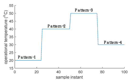
Figure 3.
Temperature profile in the PRO system in scenario 1.
In the PRO system, the temperature gradient on the heterogeneous membrane causes heat transfer inside the membrane and along the membrane surface [14]. Previous modelling and experimental studies illustrated that the temperature improvement in the feed and draw solution can simultaneously increase the osmotic pressure, the water permeability (A), solute permeability (B), diffusion coefficient (D), and mass transfer coefficient () [18]. The various parameters of solution properties, fluid mechanics, and membrane properties employed in this work are summarized in Table 3. The ICP factor is employed to demonstrate the membrane structure parameter , donating the ICP effect that occurs in the support layer. These values are case-dependent.
Table 3.
Parameters of solution properties, fluid mechanics and membrane properties. The studied draw solution is 35 g/kg (about 0.6 M) NaCl solution [16,19].
Based on the above parameters, the optimal power density values of all algorithms under temperatures fluctuations are shown in Table 4. Five existing MPPT methods, namely P&O, IMR, PSO, GWO, and WOA, are evaluated and compared with the two proposed methods (HGSO and BPSO). The optimal values are highlighted in bold. It can be observed from the table that the traditional strategies (P&O and IMR) failed to find the optimal solution and yield the lowest values. In the five existing metaheuristic-based MPPT algorithms, the performance of the PSO is worse than that of the other techniques. Among all the metaheuristic methods, the HGSO extracted the highest values in pattern 2, and the BPSO obtained the maximum power density of all the patterns.
Table 4.
Comparative analysis of the average power density extracted by different proposed MPPT algorithms under rapidly varying temperature profiles.
As illustrated in Table 5, compared with classic P&O and PSO, the proposed BPSO showed a distinct improvement of up to 6.73%. It is significant to point out that more extractable energy can be generated in the dual-stage PRO plant, and the AFI improvement of the proposed method would be more obvious.
Table 5.
Comparative analysis between the BPSO and P&O.
4.2. Scenario 2: Variations in Concentrations and Flow Rates
In this scenario, the salinity operational conditions are fluctuated, including the salinity flow rate and concentration, as shown in Figure 4.
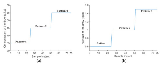
Figure 4.
Operational profiles of the salinity in the PRO system in scenario 2: (a) concentration of the draw solution; (b) flow rate of the draw solution.
The draw concentration started at 35 g/kg and then increased to 45 g/kg and 55 g/kg, respectively. In the meantime, the feed flow rate initially started at 0.6 kg/h and then increased to 1 kg/h and 1.5 kg/h, respectively. In this case study, two more novel MPPT controllers for the PRO system, namely DA and GOA, are applied and tested with the proposed BPSO method.
Similarly, the extracted optimal power density AFI and tracking rate ACT by all the algorithms of the PRO system concerning different salinities are summarized in Table 6, and the optimal values are highlighted in bold. It can be concluded from the table that the P&O obtained the smallest values in both case studies. The HGSO extracted the highest power density in pattern 2, and the BPSO showed better tracking effects than the other algorithms in all the other cases. Regarding the ACT results, the P&O method showed a relatively shorter execution time due to its simple mechanism. However, it failed to obtain an optimal AFI, leading to a low tracking efficiency. The HGSO yielded a high AFI, but the ACT value is relatively high due to its complex formulations and process. There are seven stages in the HGSO that led to a long execution time and better accuracy.
Table 6.
Comparative analysis of the extracted average power density from the different proposed MPPT controllers under rapidly changing salinity profiles, namely the draw concentrations and flow rates.
In the MPPT problem, the power efficiency mainly depends on two factors: the extractable energy and the convergence time. In Table 6, the AFI and ACT values of all eight methods under the three given salinity conditions are illustrated. The optimal values are highlighted in bold. Although all the metaheuristic algorithms had better performance than the traditional P&O method, their optimization processes are more complex, so there is a risk of longer running times. For metaheuristic strategies, a balance between exploration and exploitation is essential. The ability of the proposed BPSO to obtain the maximum power and the fastest convergence speed is proven. This is because BPSO absorbs all the advantages of the algorithms above.
The improved BPSO method enhanced the exploitation process by considering the population solutions. The detailed comparative analysis between PSO and BPSO is demonstrated in Table 7 and Figure 5. The improvement of the BPSO under three operational salinity conditions in terms of the response speed is 57.1%, 88.9%, and 36.4%, respectively. It is up to 88% better than PSO and other algorithms, which is a considerable improvement. The time increase is of significance, and the computational speed-up will enable the PRO process to be more adaptive to varying operational conditions for extracting salinity power.
Table 7.
Comparative analysis between PSO and BPSO.
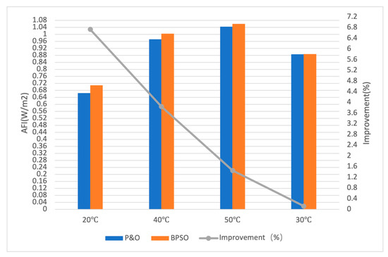
Figure 5.
Bar plot of comparative between PSO and BPSO.
5. Conclusions
For the first time, seven metaheuristic-based MPPT techniques have been employed and tested for PRO systems with various types of influential operations and salinity factors, including variations in the solution rates and concentrations and various operating temperatures based on detrimental effects. The comparative performance and the analysis of all seven methods are discussed. In this study, the classic PSO is modified to combine the essential parameters of other advanced methods. The consideration of the population solution helps to avoid the local optimal traps. The elimination of the worst solution results in reducing the search time and improving the search efficiency. The BPSO algorithm with the enhanced essential coefficients is thus proposed to boost the exploration and exploitation stage in the optimization process. From the results, the proposed BPSO-based technique overcomes the steady-state oscillations and tracking efficiency problems during the energy generation process, thereby achieving better performance regarding tracking accuracy and efficiency.
In conclusion, the BPSO method is conceived to have superior information collection and exploitation capabilities compared with other metaheuristic methods. Moreover, the analysis and comparison of the popular and recent metaheuristic methods could provide a great reference concerning the targeted method selection for different applications.
Author Contributions
Conceptualization, Y.C.; Funding acquisition, Y.C.; Investigation, Y.C.; Methodology, Y.C.; Project administration, L.G.; Supervision, L.G.; Validation, Y.C. All authors have read and agreed to the published version of the manuscript.
Funding
This research is funded by Fundamental Research Funds for the Central Universities, grant number G2021KY05123 and the Natural Science Foundation of Shaanxi Province, grant number 2020JQ-223.
Institutional Review Board Statement
Not applicable.
Informed Consent Statement
Not applicable.
Data Availability Statement
Not applicable.
Conflicts of Interest
The authors declare no conflict of interest.
Nomenclature
| current iteration | |
| velocity of the ith particle | |
| position of the ith particle | |
| w | inertia weight parameter |
| r | normalized random values in the interval (0, 1) |
| the best position found in the ith iteration | |
| the best acquired global position | |
| d | dimension |
| upper bound | |
| lower bound | |
| the mean best solution in the iteration | |
| A | membrane permeability |
| Van’t Hoff factor | |
| osmotic pressure difference between two solutions | |
| draw solution concentrations | |
| the feed solution concentrations | |
| the draw flow rates | |
| the feed flow rates | |
| mass flow rates of the permeating solution | |
| mass flow rates of the reverse solute | |
| permeate density | |
| draw solution density | |
| membrane area | |
| the permeated solution flow rate | |
| water flux | |
| salt flux | |
| salt permeability factors | |
| S | membrane structural factor |
| D | solute diffusion factor |
| osmotic pressure on the draw side | |
| osmotic pressure on the feed side | |
| solute resistivity of the porous membrane support | |
| permeate volume | |
| applied energy | |
| available extracted energy | |
| the fitness function of the designed problem | |
| the best fitness | |
| the cpu time in seconds |
References
- Loeb, S. Production of energy from concentrated brines by pressure-retarded osmosis. I. Preliminary technical and economic correlations. J. Membr. Sci. 1976, 1, 49–63. [Google Scholar] [CrossRef]
- Marin-Coria, E.; Silva, R.; Enriquez, C.; Martínez, M.L.; Mendoza, E. Environmental assessment of the impacts and benefits of a salinity gradient energy pilot plant. Energies 2021, 14, 3252. [Google Scholar] [CrossRef]
- Chen, Y.; Alanezi, A.A.; Zhou, J.; Altaee, A.; Shaheed, M.H. Optimization of module pressure retarded osmosis membrane for maximum energy extraction. J. Water Process Eng. 2019, 32, 100935. [Google Scholar] [CrossRef]
- Gonzales, R.R.; Abdel-Wahab, A.; Adham, S.; Han, D.S.; Phuntsho, S.; Suwaileh, W.; Hilal, N.; Shon, H.K. Salinity gradient energy generation by pressure retarded osmosis: A review. Desalination 2021, 500, 114841. [Google Scholar] [CrossRef]
- Alvarez-Silva, O.; Winter, C.; Osorio, A.F. Salinity Gradient Energy at River Mouths. Environ. Sci. Technol. Lett. 2014, 1, 410–415. [Google Scholar] [CrossRef]
- Long, R.; Lai, X.; Liu, Z.; Liu, W. Pressure retarded osmosis: Operating in a compromise between power density and energy efficiency. Energy 2019, 172, 592–598. [Google Scholar] [CrossRef]
- Tawalbeh, M.; Al-Othman, A.; Abdelwahab, N.; Alami, A.H.; Olabi, A.G. Recent developments in pressure retarded osmosis for desalination and power generation. Renew. Sustain. Energy Rev. 2021, 138, 110492. [Google Scholar] [CrossRef]
- He, W.; Wang, Y.; Shaheed, M.H. Maximum power point tracking (MPPT) of a scale-up pressure retarded osmosis (PRO) osmotic power plant. Appl. Energy 2015, 158, 584–596. [Google Scholar] [CrossRef] [Green Version]
- Maisonneuve, J.; Chintalacheruvu, S. Increasing osmotic power and energy with maximum power point tracking. Appl. Energy 2019, 238, 683–695. [Google Scholar] [CrossRef]
- AlZainati, N.; Saleem, H.; Altaee, A.; Zaidi, S.J.; Mohsen, M.; Hawari, A.; Millar, G.J. Pressure retarded osmosis: Advancement, challenges and potential. J. Water Process Eng. 2021, 40, 101950. [Google Scholar] [CrossRef]
- Chen, Y.; Vepa, R.; Shaheed, M.H. Enhanced and speedy energy extraction from a scaled-up pressure retarded osmosis process with a whale optimization based maximum power point tracking. Energy 2018, 153, 618–627. [Google Scholar] [CrossRef]
- Wolpert, D.H.; Macready, W.G. No free lunch theorems for optimization. IEEE Trans. Evol. Comput. 1997, 1, 67–82. [Google Scholar] [CrossRef] [Green Version]
- Miyatake, M.; Veerachary, M.; Toriumi, F.; Fujii, N.; Ko, H. Maximum power point tracking of multiple photovoltaic arrays: A PSO approach. IEEE Trans. Aerosp. Electron. Syst. 2011, 47, 367–380. [Google Scholar] [CrossRef]
- Einarsson, S.J.; Wu, B. Thermal associated pressure-retarded osmosis processes for energy production: A review. Sci. Total Environ. 2021, 757, 143731. [Google Scholar] [CrossRef] [PubMed]
- Pattle, R.E. Production of electric power by mixing fresh and salt water in the hydroelectric pile. Nature 1954, 174, 660. [Google Scholar] [CrossRef]
- He, W.; Luo, X.; Kiselychnyk, O.; Wang, J.; Shaheed, M.H. Maximum power point tracking (MPPT) control of pressure retarded osmosis (PRO) salinity power plant: Development and comparison of different techniques. Desalination 2016, 389, 187–196. [Google Scholar] [CrossRef] [Green Version]
- Van’t Hoff, J.H. The role of osmotic pressure in the analogy between solutions and gases. J. Membr. Sci. 1995, 100, 39–44. [Google Scholar] [CrossRef]
- Adhikary, S.; Islam, M.S.; Touati, K.; Sultana, S.; Ramamurthy, A.S.; Rahaman, M.S. Increased power density with low salt flux using organic draw solutions for pressure-retarded osmosis at elevated temperatures. Desalination 2020, 484, 114420. [Google Scholar] [CrossRef]
- Touati, K.; Tadeo, F.; Hänel, C.; Schiestel, T. Effect of the operating temperature on hydrodynamics and membrane parameters in pressure retarded osmosis. Desalin. Water Treat. 2016, 57, 10477–10489. [Google Scholar] [CrossRef]
Publisher’s Note: MDPI stays neutral with regard to jurisdictional claims in published maps and institutional affiliations. |
© 2021 by the authors. Licensee MDPI, Basel, Switzerland. This article is an open access article distributed under the terms and conditions of the Creative Commons Attribution (CC BY) license (https://creativecommons.org/licenses/by/4.0/).