Time-Lapse Image Method for Classifying Appliances in Nonintrusive Load Monitoring

Abstract

In this paper, a time-lapse image method is proposed to improve the classification accuracy for multistate appliances with complex patterns based on nonintrusive load monitoring (NILM). A log-likelihood ratio detector with a maxima algorithm was applied to construct a real-time event detection of home appliances. Moreover, a novel image-combining method was employed to extract information from the data based on the Gramian angular field (GAF) and recurrence plot (RP) transformations. From the simulation results, it was confirmed that the classification accuracy can be increased by up to 30% with the proposed method compared with the conventional approaches in classifying multistate appliances.

1. Introduction

Recently, various techniques have been actively investigated to optimize power consumption based on advanced metering infrastructure (AMI). An intrusive load monitoring (ILM) technique has been proposed to measure the amount of power usage by attaching a measuring terminal to each appliance load [1]. In order to alleviate the burden of installation costs for infrastructure, a nonintrusive load monitoring (NILM) technique has been proposed [2]. NILM has been expected as an energy conservation strategy by monitoring appliances in real time and conveying consumption data to users [3]. Because existing AMI can be utilized to predict power usage and classify appliances, the NILM technique can be a viable candidate for an effective solution of AMI.

However, there are challenges in identifying multistate appliances because only a few features can be extracted from a single load in the NILM technique. In order to overcome the lack of information, transforming techniques of consumption data into voltage and current (V-I) trajectory have been proposed [4,5]. However, these methods have not been realistic due to the installation costs for additional information extraction from the load.

Hidden Markov model (HMM)-based methods have been proposed to solve installation cost problems using only low-frequency data [6,7,8]. The HMM-based methods have been used to infer appliances by calculating the hidden state transition and observed state emission probabilities from a specific appliance state to another state. Despite the good classification performance of the HMM-based methods, the computational complexity of the HMM exponentially increases with the number of appliances. Therefore, the HMM-based methods have been difficult to run in real-time due to heavy computational complexity [6,7,8].

State-optimization-based approaches have been proposed to estimate optimal state transitions [9,10]. In [9], it was shown that the computation complexity can be reduced by limiting the possible appliance transition modes. Additionally, the accuracy of power consumption reconstruction has been improved by utilizing postoptimization processing [10].

In recent years, a convolutional neural network (CNN) has been employed to improve classification performance in pattern recognition and image classification [11]. The CNN algorithm has been adopted to extract features of consumption data by mapping the NILM problem into pattern recognition. Kabat et al. [12] proposed generating two-dimension (2D) feature maps for CNN using matrix rearrangement in the NILM technique. The CNN algorithm was employed to build a real-time system with a sliding window [13]. Studies applying CNN in NILM have distinguished multistate appliances well [12,13]. However, temporal information of data may be lost in the conversion process between the time-series data and matrix [12,13].

A Gramian angular field (GAF) method has been proposed to transform the time-series data into suitable formations for CNN without losing the temporal information [14]. In the GAF technique, the temporal correlations within different time intervals can be obtained from superposition and difference between different time-series data. The GAF method has shown remarkable classification performance in human activity recognition [15] and signal processing [16]. Some studies have also been conducted based on the GAF algorithm in NILM and shown good classification accuracy [17,18]. In [17], the time-series data were encoded by using the Gramian angular difference field (GADF) and Gramian angular summation field (GASF), types of GAF, to a suitable formation for CNN. The classification results of the GAF with CNN-2D have shown better performance than a model of CNN-1D with simple time-series [17]. Additionally, the results of the GAF with the denoising autoencoder (DAE) have shown better classification accuracy than the factorial hidden Markov model (FHMM) [18]. Recently, the GAF method has demonstrated good performance in combination with the stacked denoising autoencoder (sDAE) in noisy environments using real datasets [19], and it has also been utilized for short-term load forecasting [20]. However, studies using the GAF [17,18,19,20] have been simulated with only one type of GAF: the GADF or GASF transformation. The GAF technique may not typically use regression information of time-series data, which leads to the difficulty of derivations for operation patterns of appliances. Therefore, it can be said that just a fragment of the information from data has been utilized in conventional studies.

A recurrence plot (RP), also known as a recurrence graph, has recently been used in NILM [21]. The phase information of the time-series data can be captured by using the recurrence graph. In [21], the RP was used as a compressed distance similarity matrix. Additionally, appliance features were extracted by the RP. A CNN model using binary V-I images and a CNN model using RP images were compared for a benchmark. As a result of the simulation, the classification accuracy of the model using RP was improved compared with the model using binary V-I images [21]. However, the RP method [21] may not be appropriate for a practical NILM system since it is applied based on a high-frequency dataset. It is not guaranteed that all the information of time-series data has been utilized because only the RP image has been used. The phase information among various time-series data may be used in the RP image. Although amplitude information of the time-series data may affect the operational characteristics of each appliance, it may not be utilized in the RP image.

Meanwhile, various deep-learning-based methods have been proposed for the NILM approach. Classification methods based on graph signal processing (GSP) have been proposed and have shown good classification performance [22,23]. As an unsupervised approach, dynamic time warping (DTW) has been used to calculate similarities among signal patterns of appliances [22]. Graph data have been generated by using the similarities of the signal. Additionally, appliance types have been labeled by using the clustering technique in the graph data. The appliance types can be classified with deep neural networks. It has been verified that unsupervised graph signal processing with DTW (UGSP-DTW) [22] has shown outweighed classification performance compared with the conventional graph signal processing method with clustering (UGSP) [23]. However, the graph-based methods require calculating the similarities, which recur a problem of increased complexity.

As a different deep-learning approach, methods using attention modules and feature extractors have been proposed [24,25]. In [24], SCANet, a combinational method of NILM and generative adversarial network (GAN), has been presented with the GAN as a feature extractor. In [25], the load disaggregation with attention (LDwA) model was proposed. An autoencoder model with the attention module [25] was utilized to extract data features and classify appliances.

Previous works have been primarily focused on transforming the transition points of energy consumption and classifying the appliances with features of images [17,18,19,20,21]. However, these methods cannot represent all changes in the appliance. In the refrigerator, the operation of the cooler has a brief power-saving period between the temporal sequences of OFF and ON operations. The transition events of refrigerators are chronologically triggered, and subsequent events are affected by the previous operations. Therefore, to extract all the device attributes, it may be necessary to acquire features of differential values for the appliances before and after operations. In the human activity recognition (HAR) field, sequential changing features have already been utilized to improve classification accuracy by tracking changing behavioral traits [26]. Additionally, time-lapse image datasets have been used for improving classification accuracy in the biological field [27]. However, the time-lapse features have not been utilized in NILM. Therefore, the changing feature extraction of the appliance is applied to the proposed method for improving classification accuracy.

In this paper, a real-time event detection system is built by an event detection algorithm with a detection window. The existing GAF methods are supplemented by combining image data transformed by the GAF and RP transformations. A time-lapse image method is proposed to obtain detailed temporal characteristics of an appliance by approaching the NILM problem from a pattern recognition problem perspective. The contributions of the paper can be summarized in the following aspects:

• An image-combining method is proposed to transform time-series data into a suitable form for CNN and is applied to utilize most of the information in the data. Therefore, the image-combining method can be employed to supplement the existing GAF studies using only fragment information of data.
• A log-likelihood ratio detector with a maxima (LLD-max) algorithm with a denoising method is used for event detection in the proposed system. The LLD-max algorithm has been proposed for fast event detection using the detection window and local maxima [28]. Hence, a real-time event detection system can be built by applying the LLD-max algorithm.
• The time-lapse image method with an overlapping sliding window technique is proposed to extract more features of appliance data. The time-lapse image method is adopted to improve the classification accuracy of multistate appliances with complex patterns.

This paper is organized as follows. Section 2 presents the introduction of the proposed system model. Section 3 describes the algorithm principles for the proposed system model. In Section 4, simulation results of the proposed method are represented compared with the conventional methods. Finally, concluding remarks are provided in Section 5.

2. System Model

The typical and proposed NILM system models are configured in Figure 1a,b, respectively. The typical NILM system model was proposed in [2] and is represented in Figure 1a. In the first step in Figure 1a, the aggregated power is obtained by an attached meter. The measured power from the meter is defined as $M=\left\{m_1,m_2,\cdots ,m_T\right\}$, where $T$ is the largest number of given time-series data. The event detection process is performed to analyze the $M$ by decomposing the aggregated power into the power of each appliance. Additionally, the transition events are detected by the event detection algorithm. The events of power transition are represented as a unique energy consumption pattern called an appliance signature. In the feature extraction step, extracting the features of the appliance signature is performed. Finally, the extracted features are analyzed to conduct load identification.

In the proposed NILM system model, signal acquisition of the aggregated signals is performed as in the typical NILM system model. The event detection algorithm is used to detect the transition location of power usage. In the proposed model, event detection is performed in real time by the detection window technique. Unlike the typical NILM system model, loading data sequences from the transition locations and converting the data process are added as the data transformation step. By using the time-lapse image method, the converted data are linked after the data transformation step. Then, the feature extraction and load identification step can be performed by CNN with long short-term memory (CNN-LSTM) [29].

3. Algorithms for Proposed System Model

3.1. Event Detection

In event detection, it is assumed that the transition of an appliance state can be represented as a change in consumption usage. In the proposed approach, it is assumed that one appliance is activated at one event. The transition event location can be considered an operating location of each appliance. Based on this premise, transition event data are fetched by the event detection process and applied to the proposed scheme.

The LLD-max algorithm has been employed to find the transition event locations using the detection window and local maxima [28]. In the LLD-max algorithm, the transition event locations are determined by:

$$\begin{gathered} ds\left(i\right)=\frac{{\mu }_1-{\mu }_0}{{\sigma }^2}\ast \left|P\left(i\right)-\frac{{\mu }_0+{\mu }_1}{2}\right| \\ where i-W\le i\le i+W, \end{gathered}$$

(1)

$$ds\left(x\right)=\{\begin{array}{cc}\hfill ds\left(i\right),& if \left|{\mu }_1-{\mu }_0\right|>P_{th}\hfill \\ \hfill 0,& otherwise\hfill \end{array},$$

(2)

$$D_i=\max \left(abs\left(ds\left(x\right)\right)\right) ,$$

(3)

where $ds\left(i\right)$ denotes the i-th event detection result; ${\mu }_0$ and ${\mu }_1$ are the mean of the previous and post windows, respectively; ${\sigma }^2$ is the variance within the detection window; $P\left(i\right)$ is the power of the i-th selected sample; $W$ is the window size to detect local peaks; $P_{th}$ is the threshold of the chosen detection window; and $D_i$ is the i-th transition event location.

The $ds\left(i\right)$ is calculated by the mean and variance of data in the detection window as represented in Equation (1). Additionally, the $ds\left(i\right)$ is forced to be 0 if the difference between the mean value of the post and the previous windows does not exceed $P_{th}$. Here, the threshold value, $P_{th}$, is a parameter for setting the event detection sensitivity. By lowering the $P_{th}$ value, events may be detected with small variance changes within a window. Conversely, raising the $P_{th}$ value may make the event detector insensitive to small variance changes. When an appropriate value of $P_{th}$ is not selected, the classification performance may be degraded. The transition event location is detected by finding the local maximum with the absolute value of $ds\left(x\right)$ as shown in Equation (3). In Equation (2), there may be many points where the difference of mean values exceeds a predetermined threshold. Among them, the transition event location can be decided when it has the highest level of difference between mean values.

When the LLD-max algorithm is applied, the transition locations are generally well established. However, there have been cases where noise is mistaken by the transition event location [30]. Therefore, a denoising process is used to reduce such error detections and is described as follows:

$$E_i=\{\begin{array}{cc}\hfill D_i,& var\left\{P\left(X\right)\right\}\ge \left|{\mu }_1-{\mu }_0\right|\hfill \\ \hfill 0,& otherwise\hfill \end{array},D_i-\frac{W}{\mathsf{\gamma }}<X\le D_i+\frac{W}{\mathsf{\gamma }}$$

(4)

where $\mathsf{\gamma }$ denotes a constant parameter of the model and $X\in \mathbb{Z}\left(integer\right)$.

Before conducting the denoising process, it is assumed that the variance near the detected location is greater than the difference between the mean of the detection windows. In this assumption, an appropriate transition location may be selected, and the denoising process can be established. In the window, the position is removed when the variance value is below a predetermined $\left|{\mu }_1-{\mu }_0\right|$. After the denoising process, the data of the transition event locations are stored for the conversion process.

3.2. Image Transformation

The GAF [14] and RP [31] methods have been used to convert 1D time-series data into a 2D matrix suitable for CNN. When N of power measurement sequence data is given as $P=\left\{p_1,p_2,\cdots ,p_N\right\},$ the data transformation using the GAF is represented as:

$${\tilde{p}}_i{}_{\left[-1,1\right]}=\frac{\left(p_i-\max \left(P\right)\right)+\left(p_i-\min \left(P\right)\right)}{\max \left(P\right)-\min \left(P\right)},$$

(5)

$${\tilde{p}}_i{}_{\left[0,1\right]}=\frac{p_i-\min \left(P\right)}{\max \left(P\right)-\min \left(P\right)}.$$

(6)

The sampled data from $P$ in Equations (5) and (6) are normalized to values between −1 and 1 or 0 and 1, respectively. The rescaled time-series data can be represented by $\tilde{P}=\left\{{\tilde{p}}_1,{\tilde{p}}_2,\cdots ,{\tilde{p}}_N\right\}$. The samples in the rescaled time-series data can be encoded into the angular cosine as below:

$${\varnothing }_i=\arccos \left({\tilde{p}}_i\right),$$

(7)

$$GASF=\left(\begin{array}{ccc}\begin{array}{c}\cos \left({\varnothing }_1+{\varnothing }_1\right)\\ \cos \left({\varnothing }_2+{\varnothing }_1\right)\end{array}& \cdots & \begin{array}{c}\cos \left({\varnothing }_1+{\varnothing }_N\right)\\ \cos \left({\varnothing }_2+{\varnothing }_N\right)\end{array}\\ ⋮& \ddots & ⋮\\ \cos \left({\varnothing }_N+{\varnothing }_1\right)& \cdots & \cos \left({\varnothing }_N+{\varnothing }_N\right)\end{array}\right),$$

(8)

$$GADF=\left(\begin{array}{ccc}\begin{array}{c}\sin \left({\varnothing }_1-{\varnothing }_1\right)\\ \sin \left({\varnothing }_2-{\varnothing }_1\right)\end{array}& \cdots & \begin{array}{c}\sin \left({\varnothing }_1-{\varnothing }_N\right)\\ \sin \left({\varnothing }_2-{\varnothing }_N\right)\end{array}\\ ⋮& \ddots & ⋮\\ \sin \left({\varnothing }_N-{\varnothing }_1\right)& \cdots & \sin \left({\varnothing }_N-{\varnothing }_N\right)\end{array}\right),$$

(9)

where $p_i$ denotes the i-th data of $P$, and $\max \left(P\right)$ and $\min \left(P\right)$ are maximum and minimum values of sequence data $P$, respectively.

The normalized time-series data are converted to angles in Equation (7). These angles can be expressed as summation and difference as shown in Equations (8) and (9). In Equations (8) and (9), the temporal dependence is maintained as the position moves from top left to bottom right because the GAF technique can preserve the correlation property after the conversion process between time-series data and angles [14]. The GAF can be expressed in two ways—GASF and GADF—as represented in Equations (8) and (9).

The RP has been used to represent the trajectory pattern of time-series data returning to the same value in NILM [31]. In the RP, the periodic properties of an orbit can be represented by a 2D matrix [31]. The principles of the RP method is described as follows:

$$\begin{gathered} R\left(i,j\right)=\theta (ϵ-\parallel \overrightarrow{X}\left(i\right)-\overrightarrow{X}\left(j\right)\parallel ), \\ wherei,j\in \left\{1,2,\dots , T\right\}, \end{gathered}$$

(10)

$$R\left(i,j\right)=\{\begin{array}{cc}1,\hfill & if \parallel \overrightarrow{X}\left(i\right)-\overrightarrow{X}\left(j\right)\parallel \le ϵ\hfill \\ 0,\hfill & otherwise\hfill \end{array},$$

(11)

where $R\left(i,j\right)$ denotes the distance between $\overrightarrow{X}\left(i\right)$ and $\overrightarrow{X}\left(j\right)$; $\overrightarrow{X}\left(i\right)$ and $\overrightarrow{X}\left(j\right)$ are the trajectories of i-th and j-th points on the orbit in m-dimensional space, respectively; $\theta$ is the Heaviside step function; and $ϵ$ is the distance threshold.

When the data sequence $P$ is given, and m-dimension is set to be a specific dimension, then $R\left(i,j\right)$ can be calculated. From Equation (10), $R\left(i,j\right)$ is determined after passing $\theta$ by subtracting the $ϵ$ value from a distance between $\overrightarrow{X}\left(i\right)$ and $\overrightarrow{X}\left(j\right)$ [31]. Then by using Equation (11), when $\parallel \overrightarrow{X}\left(i\right)-\overrightarrow{X}\left(j\right)\parallel$ does not exceed $ϵ$, then $R\left(i,j\right)$ is equal to 1. Here, $R\left(i,j\right)=1$ means that two values in positions of $i, j$ within $P$ are closer than $ϵ$. Therefore, the m-dimensional trajectory of time-series data is calculated by Equation (11). Then 1 or 0 values are mapped into a 2D matrix according to the similarity of the distance of the trajectory. The regressed phase information of the time-series data can be contained in $R\left(i,j\right)$ by the calculation. Therefore, the RP can be utilized to supplement data information for the GAF transformation.

3.3. Time-Lapse Image Method

The proposal of the time-lapse image method can be motivated by the following two reasons: minimizing the effect of outliers and extracting unique features of multistate appliances. Due to its beneficial features, the classification accuracy can be improved for multistate appliances with complex patterns.

When the detection window becomes excessively narrow in the event detection method, the mean value within the detection window overly fluctuates. Therefore, the mean value within the detection window can become extremely large or, conversely, small. Henceforth, this phenomenon may make it difficult to find the transition locations. Thus, the range of the detection window should be increased beyond a specific size. However, the data are not well normalized due to outliers when the GAF and RP transformations are used in the large detection window. The outlier problem usually occurs because the min–max scaler in the GAF may be highly influenced by data outliers. Consequently, it has been necessary to reduce the influence of outliers while using a large detection window in the proposed method.

The multistate appliances have patterns of functioning after the operation. The patterns are essential characteristics for classifying multistate appliances. For example, the power is generated in refrigerators when the cooling function is activated and gradually decreases after the operation. When the cooling process is stopped, the power is turned off, and the amount of power is drastically reduced. In these operations, subsequent power changes are affected by the previous operations. Therefore, in classifying multistate appliances with complex patterns, it is expected that the classification accuracy can be improved by employing the changing state between operations as a feature.

The sliding window technique has been commonly used to detect anomaly transition patterns and extract features from data streams [32,33]. In [32], a causal sliding array window was used for real-time detecting anomaly detection. Additionally, a real-time detecting system was established by applying the causal sliding array window. Similarly, the sliding window technique has been used to extract short-duration variation events from the signal [33]. By applying the sliding window technique, the computational complexity can be reduced while detecting the short-duration variations. The method of the sliding window technique has also been applied to extract features in HAR [26]. In the HAR field, identifying human activity has been approached by analyzing time-series data from sensors. From the perspective of pattern recognition, the HAR problem may be similar to the NILM problem. Therefore, the sliding window technique is applied in the proposed method reflecting on the similarity of the two issues. In the time-lapse image method, the sliding window technique can be utilized to minimize the outlier effect and extract the features of multistate appliances. Here, it is empirically proven that the overlapping sliding window technique shows better classification accuracy than the nonoverlapping sliding window technique in HAR [26]. Therefore, the overlapping sliding window technique is employed for extracting features of multistate appliances.

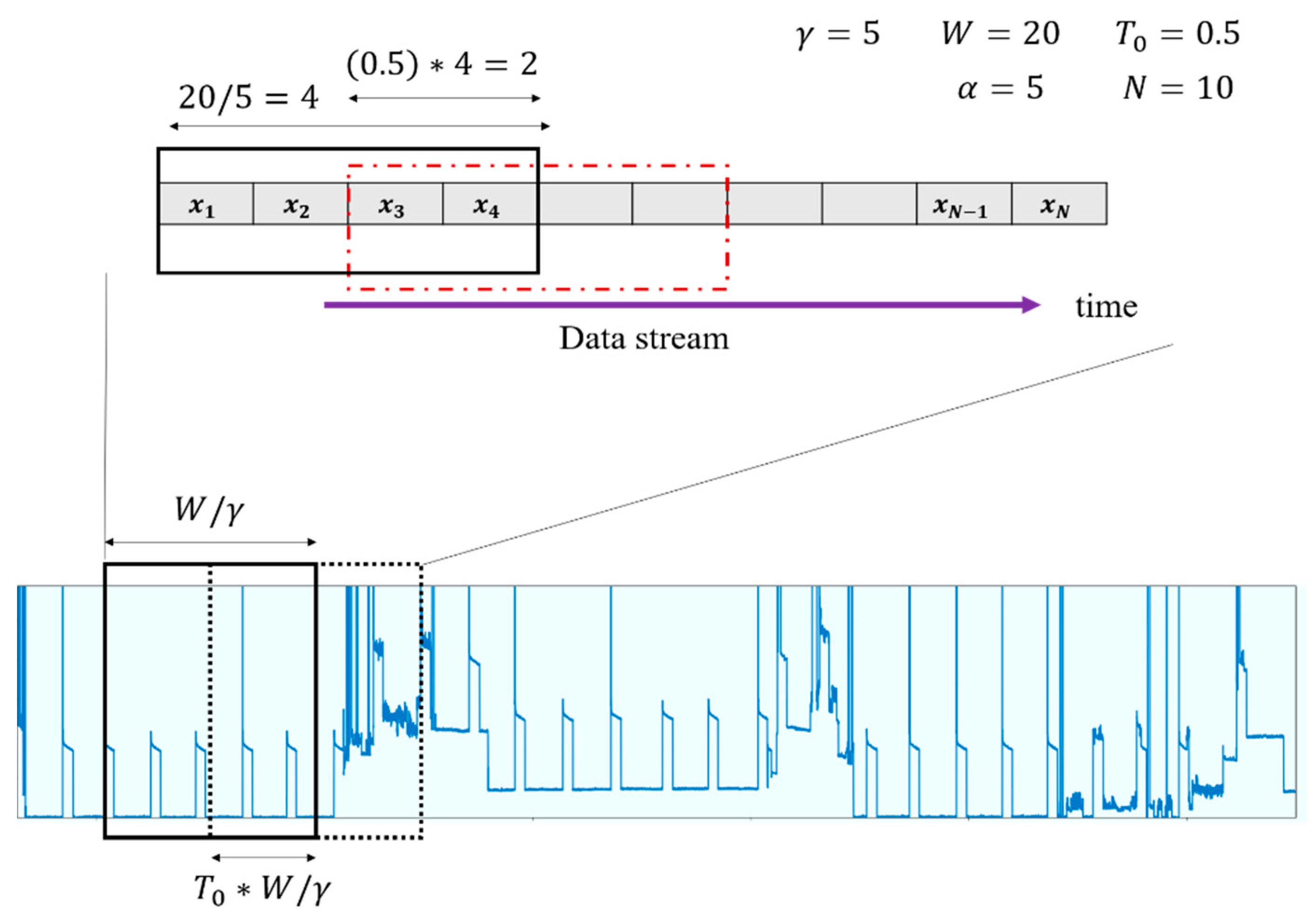
The structure of the overlapping sliding window technique in NILM can be illustrated as shown in Figure 2, where $T_0$ is the overlapping ratio. When the time-series data stream $X=\left\{x_1,x_2,\cdots x_N\right\}$ is given, a sliding window of fixed length splits each data sequence into segments, where $X$ denotes data sequences fetched from the transition locations and $N$ is the number of data samples in a segment. The data segment consisting of $N$ samples is decomposed and overlapped by the sliding window with $T_0$. Here, $T_0$ is calculated by:

$$T_0=\frac{\alpha }{N},where\alpha =\left(0,1,2,\cdots ,N-1\right).$$

(12)

The window is set to be longer than half the total length of the data stream to include the location where the event has occurred. In this paper, $T_0$ is set to 0.5 because $T_0$ is set to 0.5 in [26] and has shown good performance.

The overlapping sliding window is moved according to $T_0$. Additionally, the data sequences are stored in an array. This array is denoted as $S$. Afterward, a data normalization process is conducted with median and quartile values of $S$ to minimize the effect of outliers. This data normalization is calculated by:

$$S_{new}=\frac{S-S_{median}}{S_{75}-S_{25}},$$

(13)

where $S_{new}$ denotes normalized data, $S$ is the data in the overlapping sliding window, $S_{median}$ is the median of $S$, and $S_{75}$ and $S_{25}$ are the third and first quartile of $S$, respectively.

After the data normalization process, the image-combining method is applied. In the image-combining method, data converted by the GAF and transformed by the RP are combined. The time-series data of abundant information can be utilized by combining the transformed images. In the process of image combining, an image concatenating method is applied at the same time. The image concatenating method is employed to obtain the features of multistate appliances and improve the classification accuracy. Consequently, the time-lapse image method can be defined as transforming data by the overlapping sliding window, image-combining method, and image concatenating method together. Due to the adoption of the time-lapse image method, it is possible to reduce outlier effects and extract the attributes of multistate appliances.

The algorithm of the time-lapse image method is detailed, and some parameters are defined in the following algorithm. The $Idx$ is the location sets that are detected from the LLD-max algorithm, and it is set to be $Idx=\left\{l_1,l_2,\cdots l_N\right\}$, where $N$ is the maximum number of transition locations, and $l$ is the location from the $Idx$.

Algorithm Time-lapse image method

Input: loaded one-dimension event time-series data Output: transformed four-dimension data frame 1: Initialize $T_0$, $W$, $\gamma$, $P$ 2: Find transition event locations via (1), (2), and (3) 3: Extract $Idx$ from transition event locations via (4) 4: Load a location $l$ from the $Idx$ 5: Load event data $D$ using $l$ from $P$ 6: Set pointer $\rho =\frac{W}{\gamma }$ 7: While $\rho <W$ do 8:     Normalized event data via (12) 9:     Transform $D$ into GAF image via (8) and (9) 10:   Transform $D$ into RP image via (10) and (11) 11:   Combine the GAF and RP image data 12:   Update $\rho =\rho +\frac{W}{\gamma }\ast T_0$ 13: End while 14: Concatenate converted image frames

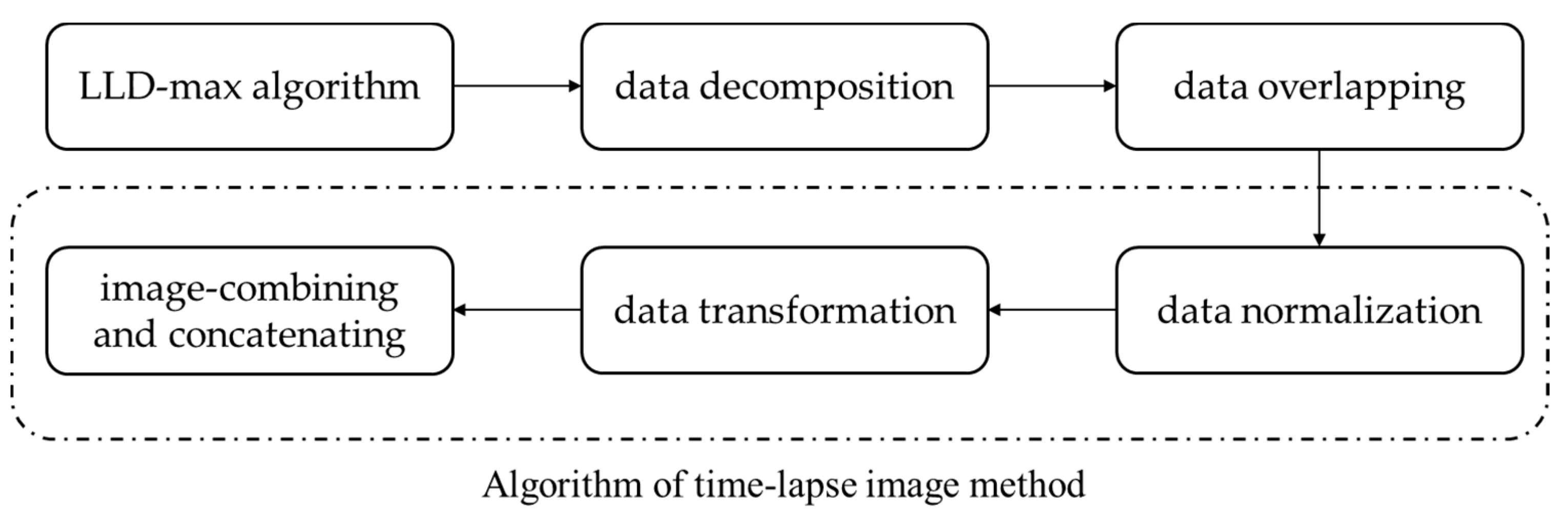
In Figure 3, a block diagram is represented for procedures of the time-lapse image method algorithm. The time-lapse image method proceeds as follows. Initially, data sequences are loaded from the locations detected by the LLD-max detector. Here, the detected points are filtered by the denoising process and stored as $P$. Afterward, the sliding window technique is applied in the loaded data sequences. Each data sequence is divided into several data segments and is overlapped by the overlapping sliding window technique. In Equation (13), the data of each segment are normalized to minimize the influence of outliers. The normalized data are converted into image frames by GAF and RP transformations. Additionally, the image frames are combined to supplement the information of each data. Afterward, adjacent combined image frames are linked in the time-sequential order of image segments. When the image concatenating process is conducted, the image frames converted by the overlapping sliding window are connected. As a result, the linked image data are structured to contain the temporal attribute and the appliance pattern before and after appliance operation.

3.4. Classification Model

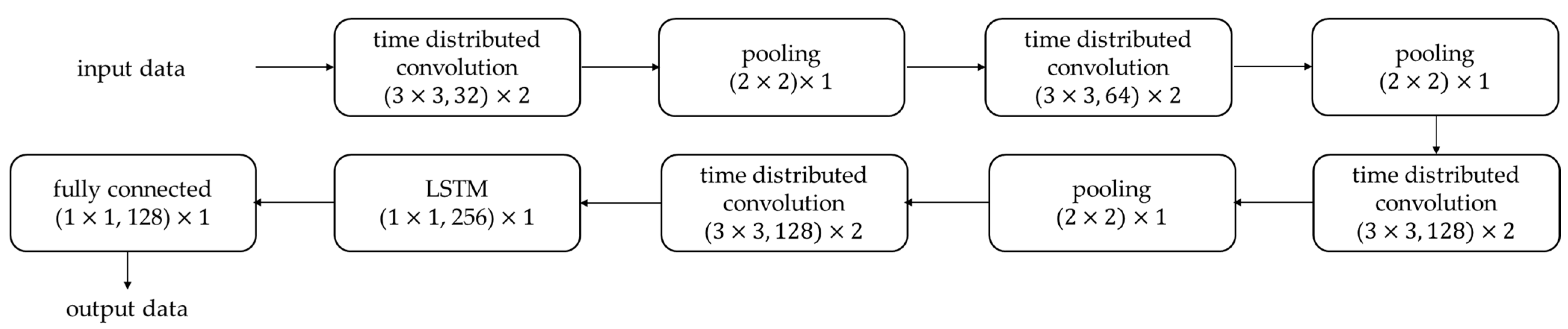
The CNN algorithm has been widely used as a deep-learning method for extracting spatial features from data. However, CNN may not be a suitable model for extracting temporal features from data [11]. The time-series data have been converted to image data in the proposed system, but the temporal features still need to be analyzed because a temporal layer has been added. Therefore, the CNN-LSTM model is adopted to extract both spatial and temporal attributes of the data. Distributed layers decompose data frames for a classification model, and feature extraction is performed with CNN layers. Then, after flattening features of the distributed layer, classification is conducted by passing the features to the LSTM and the output layers. The rectified linear unit (ReLU) [34] is used as an activation function in the layers except for the output layer. In the output layer, the sigmoid function is employed as an activation function. Additionally, binary cross entropy is employed as the loss function, and the optimizer is designed using the Adam [35]. Early stopping is used as a method to prevent overfitting. A detailed architecture with parameter values used in the simulation is represented in Figure 4. In each block, the left and right values in the bracket denote the kernel size and the number of channels, respectively. Additionally, the value outside the bracket represents the number of layers with the same structure. The number of patience for early stopping and the constant learning rate were assumed to be 10 and 0.001, respectively.

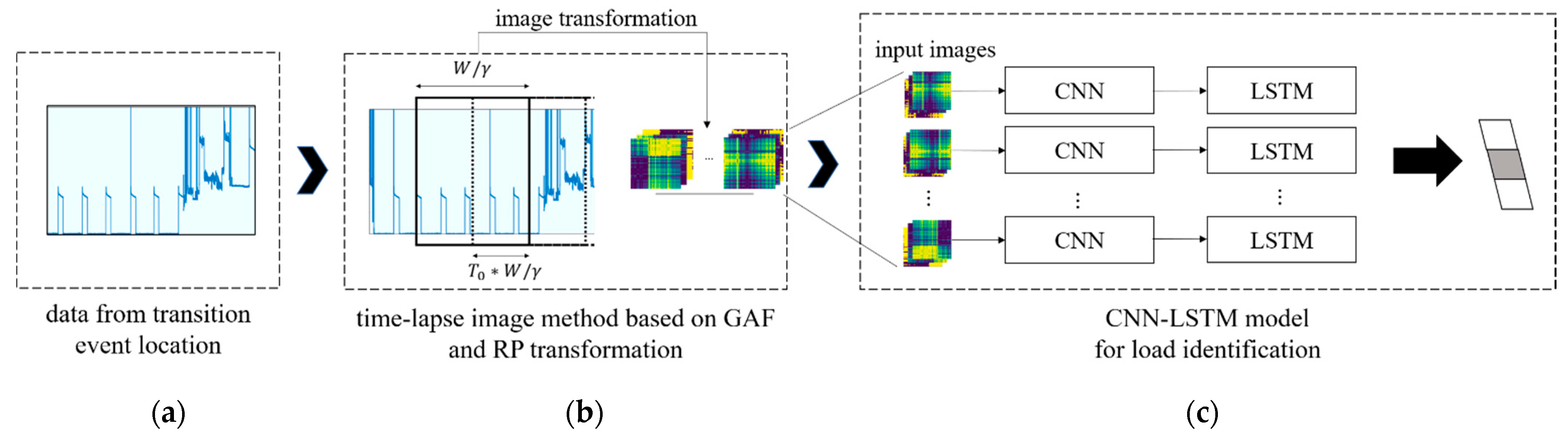
The operational process of the proposed system proceeds in the following ways. First, after conducting data preprocessing, the transition event locations are detected by the LLD-max algorithm. Then, the data are converted by the time-lapse image method. The converted data are used for training by the CNN-LSTM model. Then, the spatial and temporal features of the image data are extracted by CNN and LSTM, respectively. The operational process of the proposed system is described in Figure 5.

4. Simulation Results

Simulations have been conducted with each appliance data from aggregated power. The classification accuracy is assessed by finding a specific appliance in the aggregated power.

4.1. Dataset Setting

A residential energy disaggregation dataset (REDD) [36] was employed in the simulations. The REDD was used for NILM analysis, and each appliance was separately labeled and measured. The REDD was composed of six houses; each of the houses consisted of multistate and binary-state appliances. The multistate appliances were utilized for the simulations because the proposed method aims to enhance the classification accuracy of multistate appliances. In the simulations, refrigerators and dishwashers were selected as typical multistate appliances with complex patterns. In the REDD, houses #4, #5, and #6 were excluded because the houses had short-term data duration. Between the selected houses #1, #2, and #3, the house #1 data were used to train the system model. Houses #2 and #3 were used to confirm the performance of the system model. The training period of house #1 and the test period of other houses were set to 14-day and 10-day, respectively. From the 14-day training data, 70% of the data were set to be the training set, and the rest of the data were set to be the validation and test sets, each half, respectively.

4.2. Data Preprocessing

Aggregated power measurement sequences are fetched for the testing model, and specific appliance power sequences are extracted for the model training. The specific appliance power sequences can be denoted as $M=\left\{m_1,m_2,\cdots ,m_t,\cdots ,m_T\right\}$, where $t\in \left\{1, 2,\cdots ,T\right\}$ is time interval collected every 3 s. Additionally, the aggregated power measurement sequence data can be denoted as $P=\left\{p_1,p_2,\cdots p_T\right\}$. The transition event locations of appliances are detected by the LLD-max algorithm from $M$ and $P$. The denoising process is performed by filtering out the wrong activation locations from the event detection process. After filtering wrong locations, the transition event locations of $M$ are represented as $ID=\left\{i{d}_1,i{d}_2,\cdots , i{d}_R\right\}$, where $R$ is the maximum number of transition locations. The transition event locations of $P$ are represented as $Idx=\left\{l_1,l_2,\cdots ,l_N\right\}$. Afterward, the transition locations are employed to fetch data from $M$ and $P$. The extracted data from $M$ and $P$ are represented as $E=\left\{e_1,e_2,\cdots ,e_R\right\}$ and $K=\left\{k_1,k_2,\cdots ,k_N\right\}$, respectively. The extracted data are segmented using the sliding window technique. The data within the segment are rescaled via Equation (13). Additionally, GADF, GASF, and RP transformations have been performed on the data segments and transformed into a suitable form for CNN. Then, the three images are combined like a color channel combined with red, green, and blue (RGB). In the image-combining process, the image concatenating process is performed by linking the transformed image frames. When the concatenating process is completed, the data shape becomes the form with the time channel added.

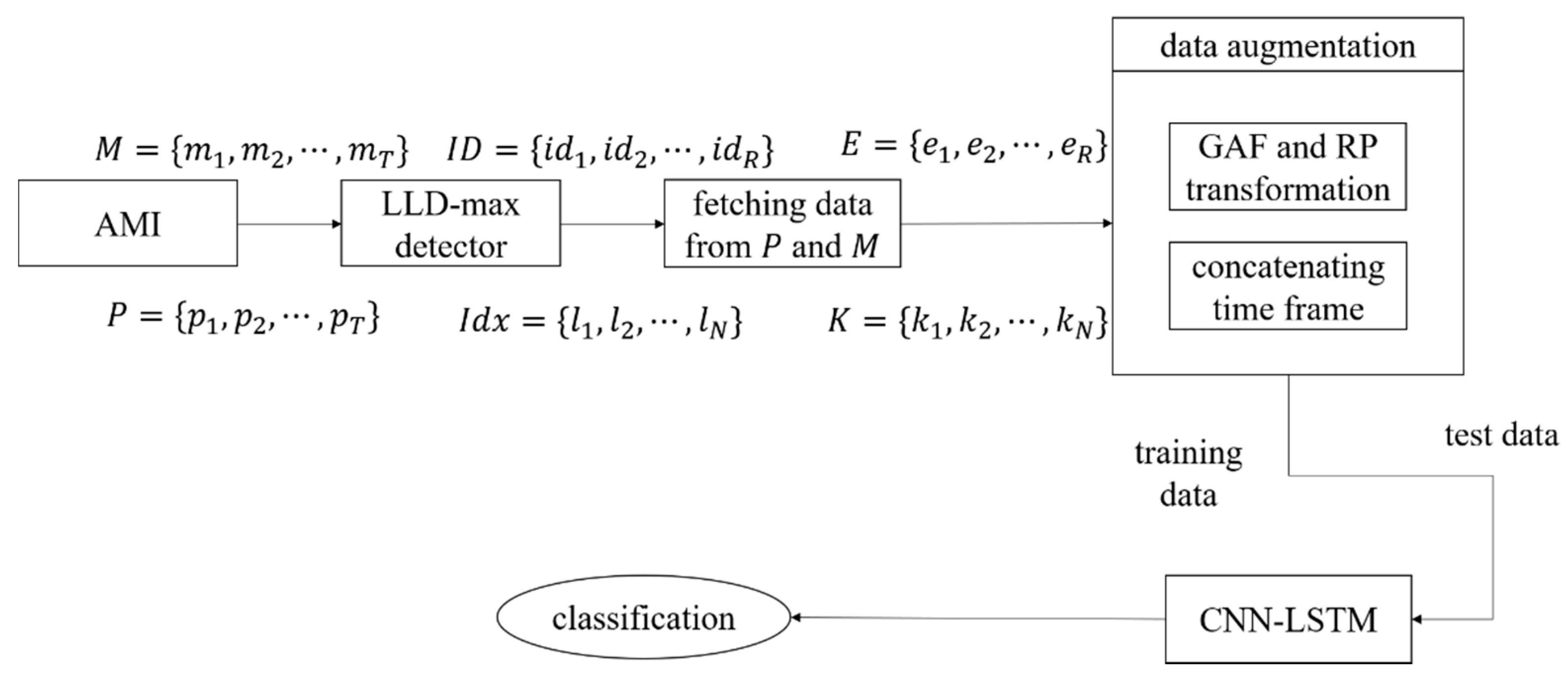
A flowchart of the proposed algorithm is represented in Figure 6. Here, the data of $E$ and $K$ are transformed into images via GAF and RP transformation. Additionally, the data augmentation is conducted with the data transformation. After all procedures, the image frames are inserted into the input data of the CNN-LSTM model. Moreover, the test data are evaluated with a generated model.

4.3. Data Augmentation

By analyzing the dataset, it has been confirmed that the dishwasher is rarely operated during the training period. In this condition, a data bias problem may be caused by the uneven operation. The biased data, also known as imbalanced data, are crucial in classification problems. Deep-learning models can be inadequately trained when imbalanced data are driven. Data augmentation techniques may be used to mitigate the data bias problem. In this paper, the time-series generative adversarial networks (TSGAN) method [37] is adopted for the data augmentation technique, a variant of generative adversarial networks (GANs) [38]. Here, the GAN is known to be able to generate realistic fake data from actual data. Additionally, a synthetic minority oversampling technique (SMOTE) [39] is applied to relieve the data bias problem. In order to mitigate the data bias problem, operating data may be generated by TSGAN and oversampled by SMOTE. The data augmentation technique is applied to the training sets only.

4.4. Performance Metrics

In the NILM technique, numerous metrics have been proposed to evaluate performance. Among the metrics, the classification accuracy can be assessed by the F1-score [40] and receiver operating characteristic (ROC) curve. The F1-score is described as the following formulas:

$$precision=\frac{tp}{tp+fp},\hspace{1em}recall=\frac{tp}{tp+fn}.$$

(14)

$$F1–score=\frac{2\times precision\times recall}{precision+recall}.$$

(15)

In Equation (14), $tp$ denotes true positives, which means that the true result is the ON state of the appliance when the prediction is ON. The $fp$ denotes false positives, which means that the prediction is the ON state of the appliance when the correct value is OFF. Additionally, the $fn$ denotes false negatives, which means that the prediction is the OFF state of the appliance when the correct value is ON.

The F1-score is a harmonic mean of precision (PC) and recall (RC) scores. The RC is the ratio of what the model predicts as true among what is true. Then the PC is the ratio of what is classified as true. The ROC curve is a graph comparing the ratio of $fp$ and the ratio of $tp$ on the $x$ and $y$ axes, respectively. The closer the ROC curve is to the upper left corner and the larger is the area occupied at the bottom, the better performance is achieved. Classification accuracy can be compared with the area of the ROC curve, where the area is called the area under the curve (AUC). The F1-score and AUC are represented as values between 0 and 1, and the larger is the value, the better is the classification performance.

4.5. Result Descriptions

The classification accuracy can be evaluated by classifying appliances in the seen and unseen houses with the model trained in house #1. Here, the test sets were aggregated data that blend consumption data from all appliances in the houses.

Before comparing the conventional studies with the proposed method, the effects of adopting the data augmentation and time-lapse image methods were analyzed. The data augmentation was applied to alleviate the problem of imbalanced operating classes of dishwashers. In Figure 7, the classification accuracy is evaluated between methods with and without data augmentation in dishwashers.

In the confusion matrix, classification accuracy is analyzed with four factors: $tp$, $tn$, $fp$, and $fn$. In Figure 7, 0 and 1 are set to be OFF and ON states, respectively. It was found that the number of $fp$ is decreased, while the number of $tp$ is increased by the adoption of the data augmentation technique. It can be interpreted that data have been less likely to be misclassified by adopting the data augmentation technique. Therefore, the classification accuracy can be improved using the data augmentation technique, which leads to the mitigation of the data bias problem.

In

Table 1. F1-score depending on time-lapse image method employment ((w): time-lapse applied, (w/o): time-lapse nonapplied).

Appliance (Method)	House #1	House #2	House #3
Dishwasher (w)	0.983	0.579	0.592
Dishwasher (w/o)	0.933	0.560	0.495
Refrigerator (w)	0.935	0.714	0.825
Refrigerator (w/o)	0.916	0.636	0.740

, the classification accuracy with and without the time-lapse image method is represented. Here, (w) and (w/o) denote the cases in which the time-lapse image method was applied and not applied, respectively. In the simulation, dishwashers and refrigerators were selected because dishwashers are typically known as multistate appliances that are difficult to classify, and refrigerators are multistate appliances found in most common households. Classification models with and without the time-lapse image method were trained by CNN-LSTM and CNN, respectively. The results confirmed that the F1-score could be improved by up to almost 10% with the time-lapse image method. It was verified that the time-lapse image method is very effective in improving classification accuracy for the appliances.

Methods in [12,17] were used to compare the classification accuracy between the conventional and proposed methods. In [12], matrix rearrangement was employed to transform a matrix suitable for CNN using time-series data. Additionally, in the case of [17], only an image of GADF or GASF was employed for classification. The conventional methods and the proposed method have been modeled with CNN and CNN-LSTM, respectively.

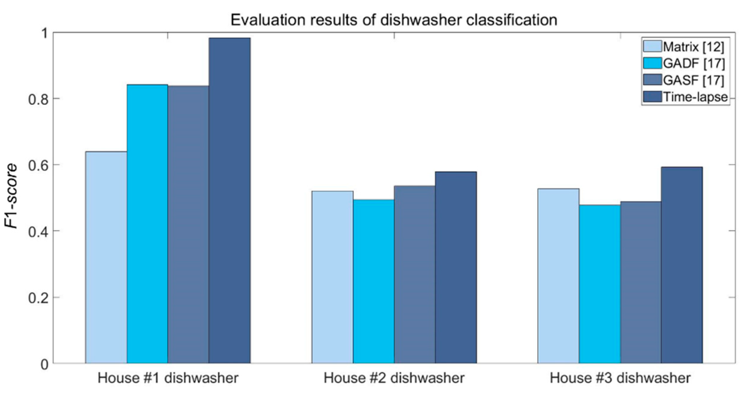
In Figure 8, the classification accuracy was simulated for dishwashers. It was shown that the GAF-based methods could improve the F1-score by up to 0.2 in house #1 compared with the matrix rearrangement method. It can be noted that the time-lapse method has been shown to improve the F1-score by up to 0.14 and 0.11, respectively, in seen and unseen houses compared with the GAF-based methods.

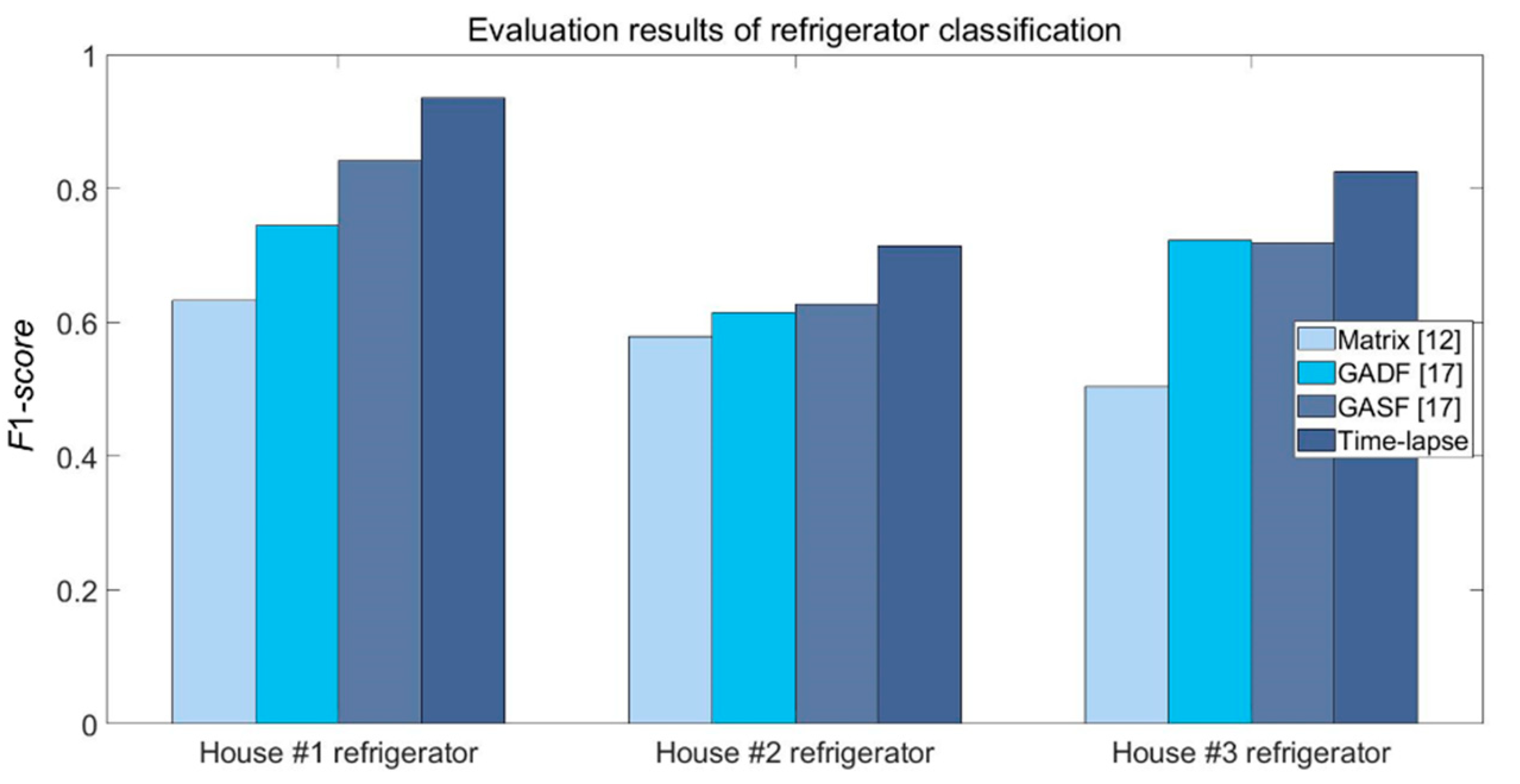
In Figure 9, the classification accuracy was simulated for refrigerators. The conventional methods can achieve an F1-score of less than 0.841 in the place where the training was conducted. It was found that the proposed method can achieve F1-score of 0.935 and 0.825 in the seen and the unseen houses, respectively.

The comparative results of the proposed and the conventional approaches are summarized in

Table 2. Simulation results of classifying multistate appliances adopting different methods.

House	Appliance	Time-Lapse Image Method			Matrix Method [12]			GADF Method [17]			GASF Method [17]
		RC	PC	F1	RC	PC	F1	RC	PC	F1	RC	PC	F1
#1	Dishwasher	0.984	0.983	0.983	0.624	0.657	0.640	0.783	0.909	0.841	0.702	0.848	0.838
(Seen)	Refrigerator	0.961	0.911	0.935	0.569	0.715	0.633	0.740	0.751	0.745	0.841	0.842	0.841
#2	Dishwasher	0.611	0.551	0.579	0.534	0.509	0.521	0.498	0.491	0.494	0.547	0.533	0.536
(Unseen)	Refrigerator	0.726	0.702	0.714	0.546	0.617	0.579	0.614	0.616	0.615	0.601	0.656	0.627
#3	Dishwasher	0.681	0.523	0.592	0.554	0.504	0.527	0.461	0.497	0.478	0.484	0.495	0.489
(Unseen)	Refrigerator	0.822	0.828	0.825	0.502	0.507	0.504	0.722	0.722	0.722	0.710	0.728	0.719

. As a result of classifying the dishwasher, it was confirmed that the time-lapse image method can improve F1-scores by up to 0.35 and 0.1 in the seen and the unseen houses, respectively, compared with the conventional approaches. Additionally, in terms of classifying the refrigerator, it was confirmed that the time-lapse image method can also improve F1-scores by up to 0.3 and 0.32 in the seen and the unseen houses, respectively, compared with the conventional methods.

In Figure 10, the ROC curves are represented for the dishwasher with AUC. It was verified that AUC scores can be improved by up to 0.54 and 0.37 in the seen and the unseen houses, respectively, compared with the conventional methods.

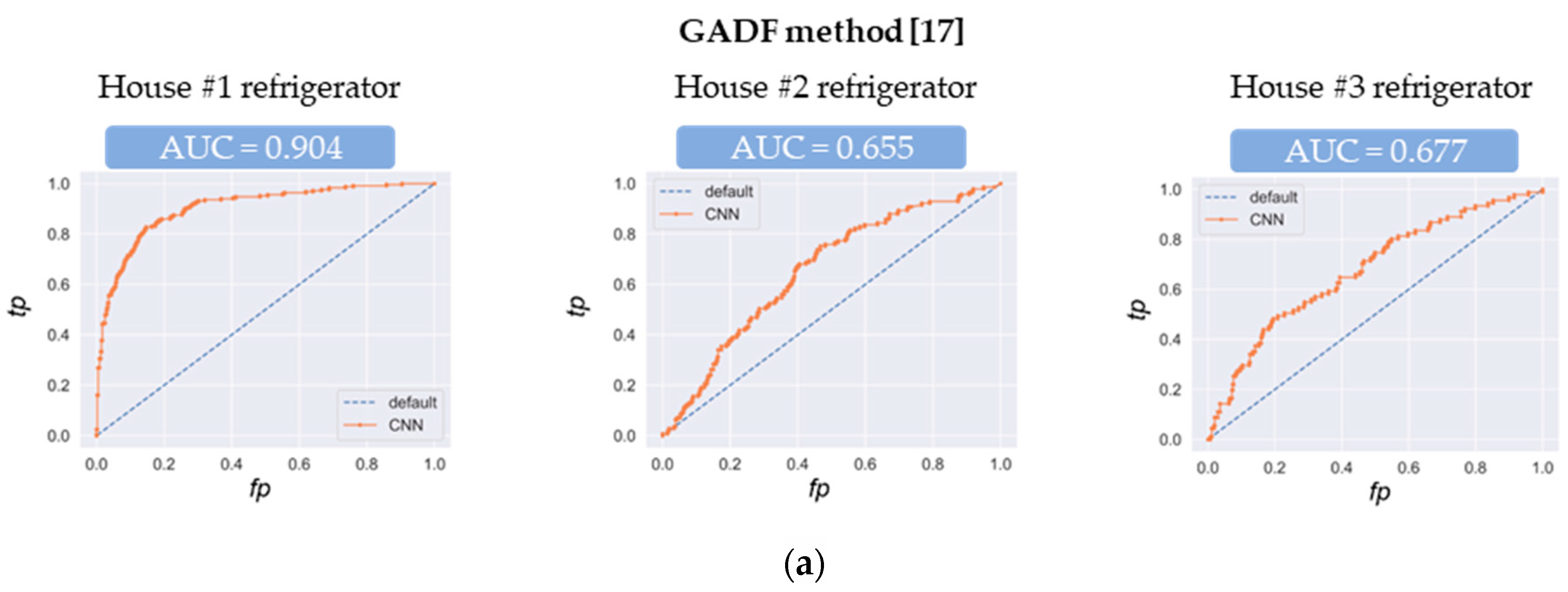
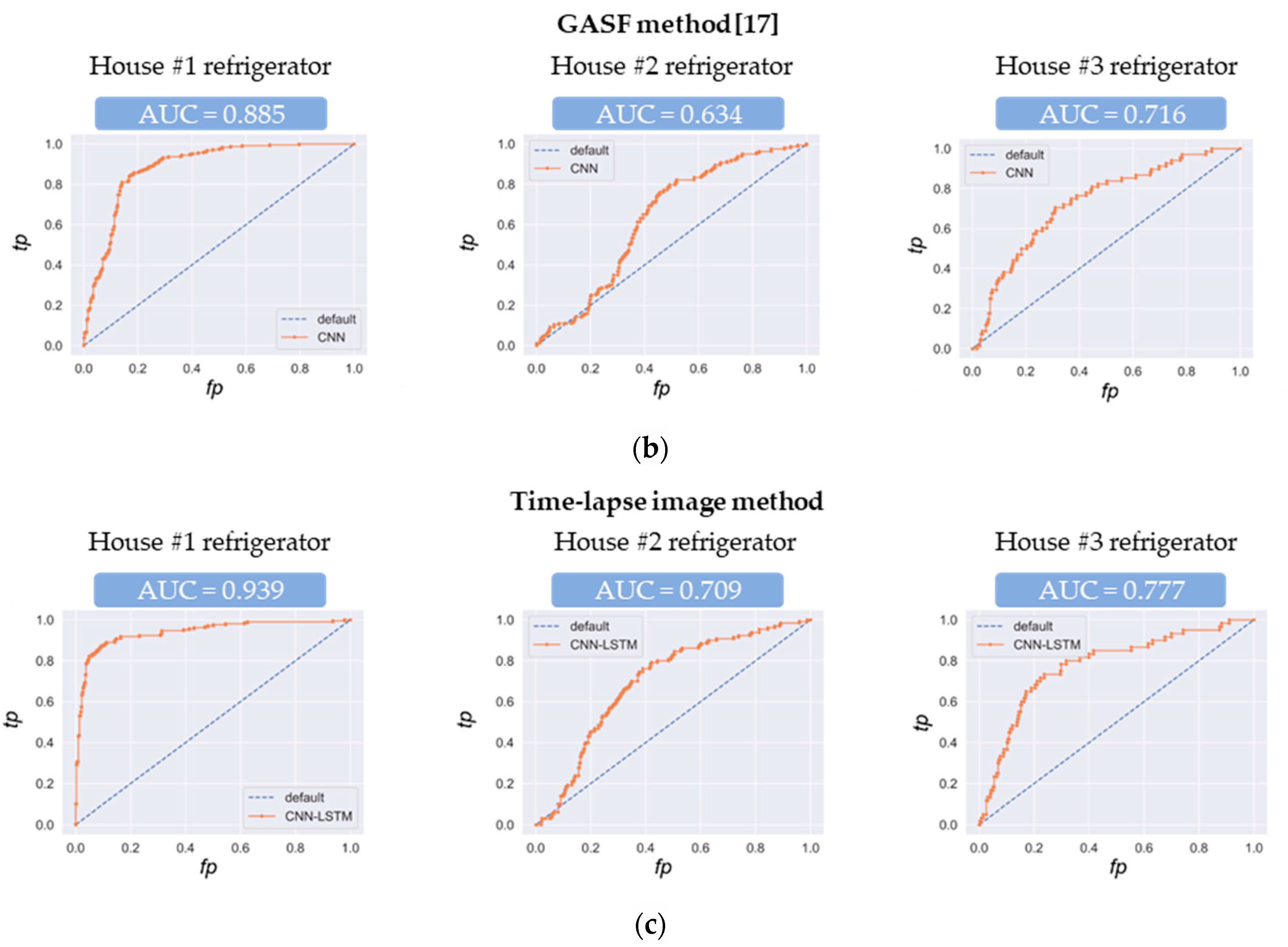
In Figure 11, the ROC curves are represented for the refrigerator with AUC. By the proposed approach, it was noted that AUC scores can be improved by up to 0.349 and 0.251 in the seen and the unseen houses, respectively, compared with the conventional methods.

In terms of the F1-score and ROC curve, it was verified that the classification accuracy was significantly enhanced by the time-lapse image method compared with the conventional approaches.

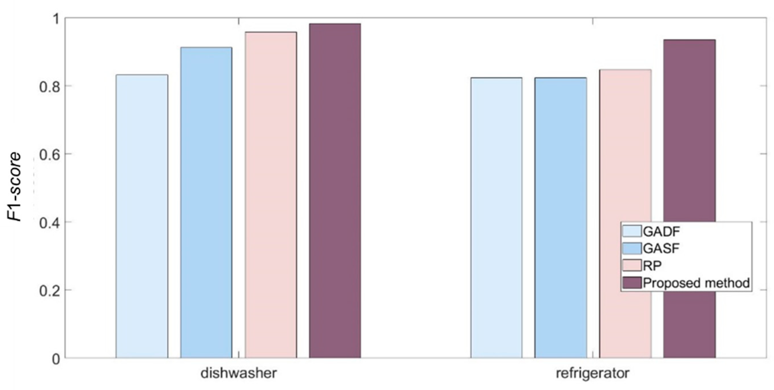
In Figure 12, the simulations were performed for dishwashers and refrigerators in terms of F1-score. It was confirmed that the classification accuracy can be improved by combining the RP and GAF techniques compared with each technique.

In

Table 3. Recall (RC)/precision (PC)/F1-score (F1) for the proposed and conventional deep-learning methods.

House	Appliance	Time-Lapse Image Method			CNN-1D Method			RF Method
		RC	PC	F1	RC	PC	F1	RC	PC	F1
#1	Dishwasher	0.984	0.983	0.983	0.484	0.461	0.472	0.263	0.625	0.370
(Seen)	Refrigerator	0.961	0.911	0.935	0.538	0.667	0.596	0.485	0.662	0.560
#2	Dishwasher	0.611	0.551	0.579	0.5	0.49	0.495	0.511	0.507	0.509
(Unseen)	Refrigerator	0.726	0.702	0.714	0.507	0.591	0.546	0.673	0.652	0.662
#3	Dishwasher	0.681	0.523	0.592	0.492	0.498	0.495	0.509	0.501	0.505
(Unseen)	Refrigerator	0.822	0.828	0.825	0.505	0.615	0.555	0.591	0.652	0.620

, the proposed method is compared with the traditional deep-learning methods in terms of RC, PC, and F1-score. The CNN-1D and random forest (RF) methods are chosen as representative deep-learning methods. The proposed method can improve the F1-scores of dishwashers and refrigerators by up to 0.61 and 0.37, respectively, compared with the traditional deep-learning methods. Therefore, the time-lapse image method can be a promising candidate for enhancing classification accuracy from the standpoint of F1-scores.

In order to evaluate the classification accuracy between the time-lapse image and recent other deep-learning methods [22,23,24,25], F1-scores for REDD house #1 are represented in

Table 4. F1-score of deep-learning methods for REDD house 1.

Appliance	Setting 1			Setting 2
	Time-Lapse Image	UGSP-DTW [22]	UGSP [23]	Time-Lapse Image	LDwA [24]	SCANet [25]
Dishwasher	0.97	0.77	0.62	0.79	0.74	0.69
Refrigerator	0.95	0.92	0.85	0.89	0.87	0.83

. For setting similar simulation environments, which were conducted in the deep-learning methods [22,23,24,25], settings were divided into a couple of settings: settings 1 and 2. In setting 1, houses #2, #3, #4, #5, and #6 were used as training data, and house # 1 was used as test data. In setting 2, house #1 was used as the training data, and the validation data of house # 1 was classified. From the simulation results of setting 1, it was confirmed that the F1-scores of the dishwashers and refrigerators can be improved by up to 0.35 and 0.1, respectively, compared with the conventional GSP methods [22,23]. From the simulation results of setting 2, it was confirmed that the F1-score of dishwashers and refrigerators can be improved by up to 0.1 and 0.06, respectively, compared with the conventional feature extraction methods [24,25]. Therefore, it was verified that the time-lapse image method is very effective for the enhancement of classification accuracy compared with the recently adopted methods.

5. Conclusions and Discussions

In this paper, the LLD-max algorithm was applied to construct a real-time event detection of typical home appliances. The novel image-combining method was proposed to extract features based on the GAF and RP transformations. Additionally, the time-lapse image method was proposed to improve the classification accuracy for multistate appliances with complex patterns. It can be noted that the bias data problem may be mitigated with the data augmentation technique. It was confirmed that the classification accuracy measured by the F1-score can be enhanced by up to 30% or more through the proposed method. Consequently, it was confirmed that the proposed method can achieve enhanced classification accuracy compared with the conventional methods in classifying the multistate appliances. The proposed technique can find its applications in energy-saving and management systems with various home appliances.