Optimal Integrated Emission Management through Variable Engine Calibration

Abstract

In this work, the potential for improving the trade-off between fuel consumption and tailpipe NO_x emissions through variable engine calibration (VEC) is demonstrated for both conventional and hybrid electric vehicles (HEV). First, a preoptimization procedure for the engine operation is proposed to address the challenge posed by the large number of engine control inputs. By excluding infeasible and suboptimal operation offline, an engine model is developed that can be evaluated efficiently during online optimization. Next, dynamic programming is used to find the optimal trade-off between fuel consumption and tailpipe NO_x emissions for various vehicle configurations and driving missions. Simulation results show that for a conventional vehicle equipped with VEC and gear optimization run on the worldwide harmonized light vehicles test cycle (WLTC), the fuel consumption can be reduced by 5.4% at equivalent NO_x emissions. At equivalent fuel consumption, the NO_x emissions can be reduced by 80%. For an HEV, the introduction of VEC, in addition to the optimization of the torque split and the gear selection, drastically extended the achievable trade-off between fuel consumption and tailpipe NO_x emissions in simulations. Most notably, the region with very low NO_x emissions could only be reached with VEC.

1. Introduction

In recent decades, the introduction of ever more stringent pollutant emission limits led to the widespread introduction of exhaust gas aftertreatment systems (ATS) in vehicles [1,2]. The introduction of CO₂ limits in recent years has further resulted in a rise in the number of hybrid electric vehicles (HEV) [3,4]. As a result, the number of components in modern powertrains has grown. To exploit the full potential of these powertrains, a high-level controller is required that manages the interactions of the individual components and maximizes the performance of the powertrain as a whole. This controller is typically referred to as a supervisory controller [5].

1.1. Literature Review: Optimal Powertrain Control

The optimal energy management of HEVs has been intensively researched, as shown by the overview presented in [6]. The equivalent consumption minimization strategy (ECMS) was identified as the most promising supervisory control approach. The method relies on simplifying the optimal control problem (OCP) to an instantaneous optimization for a mission-dependent constant equivalence factor that translates the cost of using electric energy to an equivalent fuel cost. The value of the equivalence factor can be determined based on predictive mission information and is adapted online to correct for model mismatch and disturbances [5].

Recently, this method was adapted to account for engine-out emissions. In [7], a conventional powertrain equipped with a diesel engine whose start of injection can be optimized during operation was considered. ECMS was applied to the optimal emission management problem by introducing an equivalent cost factor that translates engine-out NO_x emissions to an equivalent fuel cost. In [8], the combined energy and emission management problem was tackled for an HEV. The resulting methods were found to work well when no ATS was considered.

The pollutant reduction efficiency of an ATS depends strongly on its temperature [2]. The selective catalytic reduction (SCR) catalysts used to reduce NO_x emissions of diesel-powered vehicles are especially sensitive to this behavior. As shown in [9], the thermal dynamics of the ATS have a strong impact on the optimal operation of the vehicle. ECMS approaches based on equivalence factors that are constant over the mission can no longer be applied, and new control methods are required.

For conventional vehicles that allow the engine calibration to be varied online, the fuel consumption, engine-out NO_x emissions, and exhaust enthalpy can be influenced during operation [10,11,12,13,14,15,16]. In this setting, the task of the supervisory controller is to set the engine operation such that the fuel consumption is minimized while a tailpipe NO_x limit is not exceeded. As the engine operation chosen affects the evolution of the ATS temperature and therefore its NO_x-reduction efficiency, the thermal ATS dynamics must be considered by the supervisory controller. In [10,11], an ECMS-like approach is proposed that uses a heuristic method to approximate the non-constant ATS temperature equivalence factor, depending on the current ATS temperature. In [12,13], a two-level model predictive control (MPC) structure was used to optimize the operation of the engine and the ATS online.

In HEVs, the torque split between the combustion engine and the electric propulsion components can be used to optimize the overall fuel consumption and emissions. In [17,18], dynamic programming (DP) was used to find the optimal operation offline. In [19], a real-time capable optimization method to solve the problem was presented. In [20], an ECMS-like approach was used to control the battery equivalence factor and the tailpipe NO_x equivalence factor, and a heuristic method was used to determine the ATS temperature equivalence factor. In [21], the ATS temperature equivalence factor was found as the dual variable of an offline optimization, and a look-up table was developed that returns its value depending on the current ATS temperature and the tailpipe NO_x equivalence factor. In [22,23,24], MPC approaches were presented that optimize performance through online optimization. For all of the examples above, the engine calibration was considered to be fixed. While only the torque split was optimized in [18,20,21,22,23,24], the gear selection and the engine on/off decisions were further considered in [17,19].

The publications listed above optimize either the operation of the combustion engine, i.e., the inputs to the engine itself, or that of the HEV powertrain, i.e., the torque split, the gear selection, and the engine on/off decisions. Furthermore, while publications that focus purely on energy management are abundant, publications that include emissions and ATS considerations are much scarcer. To the best of the authors’ knowledge, no study exists that jointly optimized the operation of a parallel-hybrid vehicle and the operation of an engine whose calibration can be varied online while accounting for the ATS temperature and the pollutant emissions. The closest example in the literature is [25], where a vehicle equipped with a waste heat recovery system was considered, and the engine operation and the power drawn from the battery were optimized jointly. However, the degree of hybridization was extremely small, and no regenerative braking was considered. As a result, the full potential of a diesel-electric parallel-hybrid vehicle equipped with a variable engine calibration (VEC) and an ATS is undocumented as of yet.

1.2. Literature Review: Preoptimization of Engine Operation

As will be shown in this paper, the more engine control inputs that can be varied during operation, the better the engine operation can be tailored to the specific mission and the better the overall performance regarding fuel consumption and pollutant emissions will be. It is therefore useful to allow variation in all engine control inputs that affect the engine operation in a way that influences the overall objective. Unfortunately, the resulting OCP becomes more challenging if more engine control inputs are considered. This is likely the reason why, in the literature, a limited number of engine control inputs are considered. A single engine control input was considered in [7], two in [10,11,14], three in [12,15,16], and four in [13].

To deal with the high-dimensional control problem resulting from considering many engine control inputs, some researchers applied a preoptimization to reduce the dimensionality of the supervisory control problem [14,15,16]. First, a set of objectives is defined for a multi-objective optimization of the engine operation. Next, the Pareto-optimal operation for this multi-objective optimization is identified from the range of feasible input combinations. If the number of objectives is smaller than the number of engine control inputs considered, the resulting Pareto front can be seen as a reduced-order model of the engine that a priori excludes all input combinations that are known to be suboptimal. In the supervisory control problem, the decision variables are no longer the engine control inputs, but the individual objectives of the multi-objective engine optimization, termed engine strategy inputs.

In [14,15], the trade-off between fuel consumption and engine-out NO_x emissions is considered. In [15], three engine control inputs were taken into account and a Pareto front mapping the specified NO_x limit to the resulting fuel consumption was identified. The three engine control inputs were reduced to a single engine strategy input, namely, the position on the Pareto front, resulting in an order reduction by two dimensions. In [16], the operation of the engine with three engine control inputs was mapped to a Pareto front describing the trade-off between fuel consumption, engine-out NO_x, and engine-out particulate matter. All approaches found in the literature define a hypercube in the input space in which the engine operation must be feasible, i.e., where no engine limits are violated. This hypercube of feasible inputs is then used as the input space considered. While this approach avoids having to deal with infeasible engine operation at feasible input combinations, it restricts the operation of the engine and likely results in a suboptimal operation. Moreover, none of the works cited above consider the effect of the engine operation on the ATS temperature and therefore on the future NO_x-reduction efficiency during the optimization of the engine operation.

1.3. Contribution

The contribution of this work is twofold. First, a systematic method to perform a preoptimization of the engine operation is presented, which results in an order reduction of the supervisory control problem. Specifically, five engine control inputs are considered in the preoptimization that identifies the Pareto front spanned by the fuel consumption, the engine-out NO_x emissions, and the enthalpy flow to the ATS. Unlike in previous publications, the engine control inputs are not limited to a feasible hypercube, but could span the full range of feasible inputs. Second, the potential of a supervisory controller taking into account pollutant emissions and the ATS for a powertrain with VEC is evaluated using DP optimization. Both conventional vehicles and HEVs are considered. Simulation results show that the introduction of VEC drastically extends the achievable trade-off between fuel consumption and tailpipe NO_x emissions for both conventional vehicles and HEVs.

1.4. Structure

In Section 2, the vehicle considered is described. In Section 3, the engine preoptimization methodology is introduced. In Section 4, the OCP is formulated and the DP optimization procedure is introduced. The results for a conventional vehicle are presented in Section 5, and those for an HEV are presented in Section 6. Finally, in Section 7, conclusions are drawn and an outlook to future research is given.

2. Problem Description

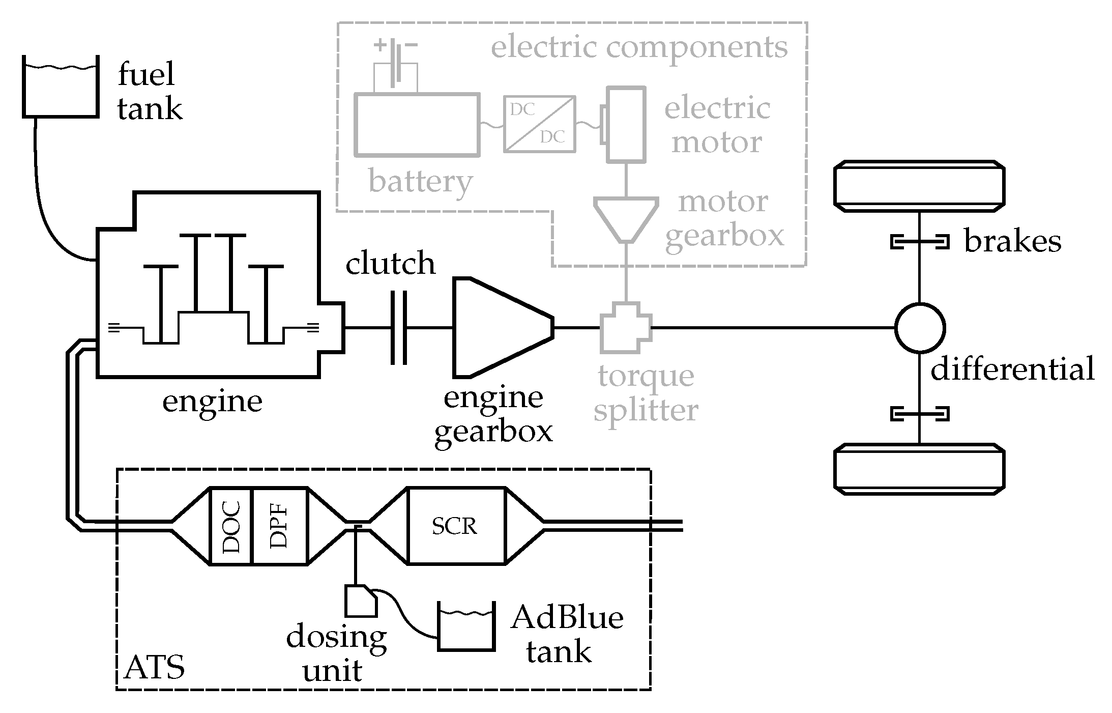
The parallel-hybrid powertrain considered in this work is shown in Figure 1. In Section 5, a conventional vehicle featuring the components shown in black is considered. It is powered by a diesel engine connected to the propeller shaft via a clutch and a six-speed automatic gearbox. It further features an ATS consisting of a diesel oxidation catalyst (DOC), a diesel particulate filter (DPF), and a selective catalytic reduction (SCR) system. In Section 6, an HEV is considered which additionally features the electric components shown in gray. A single electric machine is connected to the torque splitter via a fixed-transmission-ratio gearbox. It draws power from the battery via a DC–DC converter.

2.1. Powertrain Model

The modeling approach used for the vehicle dynamics and the electric components is based on [5]. Only a minimal description of the vehicle model is given here, as further details can be found in [19,26]. Numerical values for the main powertrain data are provided in Appendix A.

Given the vehicle speed v, the acceleration a, and the road gradient $\mathsf{\Gamma }$, the speed and torque at the output of the torque splitter are

$$\begin{array}{cc}\hfill {\omega }_{\mathrm{ts}}& =\frac{{\gamma }_{\mathrm{fd}}}{r_{\mathrm{w}}}v\hfill \end{array}$$

(1)

$$\begin{array}{cc}\hfill T_{\mathrm{ts}}& =\frac{r_{\mathrm{w}}}{{\gamma }_{\mathrm{fd}}}\left(F_{\mathrm{d}}(\mathsf{\Gamma },v)+F_{\mathrm{m}}\left(a\right)+F_{\mathrm{br}}\right),\hfill \end{array}$$

(2)

where ${\gamma }_{\mathrm{fd}}$ is the final drive ratio of the differential gearbox, $r_{\mathrm{w}}$ is the wheel radius, $F_{\mathrm{m}}$ is the inertial force, and $F_{\mathrm{br}}$ is the force applied by the brakes. The drag force $F_{\mathrm{d}}$ consists of the aerodynamic drag, the rolling resistance, and the gravitational force.

The torque split u sets the torque to be provided at the torque splitter by the motor $T_{\mathrm{m},\mathrm{ts}}$ and the engine $T_{\mathrm{e},\mathrm{ts}}$, respectively.

$$\begin{array}{cc}\hfill T_{\mathrm{m},\mathrm{ts}}& =u{T}_{\mathrm{ts}}\hfill \end{array}$$

(3)

$$\begin{array}{cc}\hfill T_{\mathrm{e},\mathrm{ts}}& =(1-u)T_{\mathrm{ts}}\hfill \end{array}$$

(4)

The motor gearbox and the DC–DC converter are modeled using a constant efficiency. The motor efficiency is given as a map of the motor speed and torque. The battery is modeled using an equivalent circuit model, where both the open-circuit voltage and the internal resistance depend on the battery state of charge. The dynamics of the state of charge $\xi$ are

$$\dot{\xi }=-\frac{I_{\mathrm{b}}({\omega }_{\mathrm{m}},T_{\mathrm{m}},\xi )}{Q_{\max }},$$

(5)

where $I_{\mathrm{b}}$ is the current drawn from the battery, which depends on the motor speed ${\omega }_{\mathrm{m}}$, the motor torque $T_{\mathrm{m}}$, and the state of charge. The maximum capacity of the battery is given by $Q_{\max }$. Upper and lower constraints on the motor torque, the battery current, and the state of charge are considered.

The engine gearbox is modeled using a constant efficiency. Upper and lower constraints on the engine torque are considered. The engine model will be outlined in the next section.

The thermal model of the ATS consists of a single lumped brick temperature $\vartheta$, whose dynamics are

$$\begin{array}{cc}\hfill \dot{\vartheta }& =\frac{{\stackrel{*}{H}}_{\mathrm{ATS}}-{\stackrel{*}{Q}}_{\mathrm{hl}}}{C_{\mathrm{ATS}}}\hfill \end{array}$$

(6)

$$\begin{array}{cc}\hfill {\stackrel{*}{H}}_{\mathrm{ATS}}& ={\stackrel{*}{m}}_{\mathrm{exh}}{c}_{\mathrm{p}}({\vartheta }_{\mathrm{exh}}-\vartheta )\hfill \end{array}$$

(7)

$$\begin{array}{cc}\hfill {\stackrel{*}{Q}}_{\mathrm{hl}}& =\alpha S(\vartheta -{\vartheta }_{\mathrm{amb}}),\hfill \end{array}$$

(8)

where $C_{\mathrm{ATS}}$ is the thermal inertia of the ATS and ${\stackrel{*}{m}}_{\mathrm{exh}}$ is the exhaust mass flow. The enthalpy flow from the exhaust gas to the ATS is denoted by ${\stackrel{*}{H}}_{\mathrm{ATS}}$, where $c_{\mathrm{p}}$ is the specific heat capacity of the exhaust gas and ${\vartheta }_{\mathrm{exh}}$ is the exhaust gas temperature. The conductive heat loss to the environment is denoted by ${\stackrel{*}{Q}}_{\mathrm{hl}}$, where $\alpha$ is the heat transfer coefficient, S is the outer surface area of the ATS, and ${\vartheta }_{\mathrm{amb}}$ is the ambient temperature.

The chemical model of the ATS consists of a static look-up table which gives the NO_x-reduction efficiency ${\eta }_{\mathrm{DeNOx}}$ as a function of the ATS temperature and the exhaust mass flow. The tailpipe NO_x mass flow is

$${\stackrel{*}{m}}_{{\mathrm{NO}}_{\mathrm{x}}}^{\mathrm{tp}}=\left(1-{\eta }_{\mathrm{DeNOx}}(\vartheta ,{\stackrel{*}{m}}_{\mathrm{exh}})\right){\stackrel{*}{m}}_{{\mathrm{NO}}_{\mathrm{x}}}^{\mathrm{eo}},$$

(9)

where ${\stackrel{*}{m}}_{{\mathrm{NO}}_{\mathrm{x}}}^{\mathrm{eo}}$ is the engine-out NO_x mass flow.

2.2. Control Task

The vehicle mission is assumed to be given and has to be followed exactly. The system has two dynamic states, namely, the battery state of charge $\xi$ and the ATS temperature $\vartheta$.

The objective of the control task considered in this work is to minimize the fuel consumed by the vehicle. During the mission two operational constraints must be satisfied. First, a charge-sustaining operation is demanded—i.e., the battery state of charge at the end of the mission must be at least as high as at the beginning. Second, a given upper bound on the emitted tailpipe NO_x mass must not be exceeded at the end of the mission. As the ATS temperature has a strong impact on the NO_x-reduction efficiency and therefore on the tailpipe NO_x emissions, it must be carefully managed along the mission.

In Section 4.1, a rigorous mathematical formulation of the optimal control problem is stated, which accounts for the engine preoptimization introduced in the next section.

3. Engine Preoptimization

Modern combustion engines have many engine control inputs that affect their operation—i.e., fuel consumption, engine-out pollutant emissions, exhaust enthalpy, etc. As they are generally over-actuated, some engine control inputs can be optimized online to adapt the engine operation for the current conditions. In the following, the engine control inputs that can be optimized during operation are referred to as degrees of freedom (DoF).

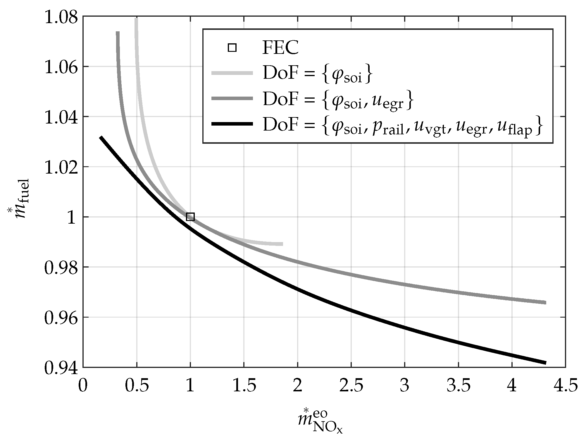
In general, the more DoF available, the better the achievable engine performance. Figure 2 shows the achievable trade-off between fuel consumption and engine-out NO_x emissions for different sets of DoF, at fixed engine speed and torque. The operation with a fixed engine calibration (FEC), i.e., no DoF, is shown by the rectangular marker. The light gray curve shows the trade-off when the start of injection ${\phi }_{\mathrm{soi}}$ was considered as the sole DoF. Even with a single DoF, a considerable range in engine operation becomes available. When the position of the exhaust gas recirculation (EGR) valve was included as a second DoF, the dark gray trade-off curve resulted. The Pareto-optimal region was extended significantly. When the fuel rail pressure $p_{\mathrm{rail}}$, the variable geometry turbine (VGT) actuator position $u_{\mathrm{vgt}}$, and the exhaust flap position $u_{\mathrm{flap}}$ were added to the list of DoF, the black trade-off curve resulted.

In this work, five DoF were considered, namely, the start of injection, the fuel rail pressure, the VGT actuator position, the EGR valve position, and the exhaust flap position. However, the presented preoptimization method is easily transferable to systems with different DoF.

The presented engine preoptimization method is based on the concept of Pareto-optimality for a multi-objective optimization [27]. The goal of the preoptimization is to exclude all engine control input combinations that either result in an infeasible engine operation, i.e., where at least one engine constraint is violated, or in an engine operation that is not Pareto-optimal.

Before starting the engine preoptimization, the individual objectives of the multi-objective optimization must be defined. The control task defined in Section 2.2 clearly states that the fuel consumption is to be minimized. Further, the engine-out NO_x mass flow is to be minimized, in order to meet the limit on the emitted tailpipe NO_x. Due to the NO_x-reduction efficiency of the ATS increasing as its temperature rises, the enthalpy provided to the ATS is to be maximized. In this work the enthalpy provided to the ATS, the engine-out NO_x mass flow, and the fuel mass flow are considered as the objectives for the engine preoptimization. The exhaust mass flow, which is required to evaluate the ATS NO_x-reduction efficiency, is considered as an output depending on the engine operation selected.

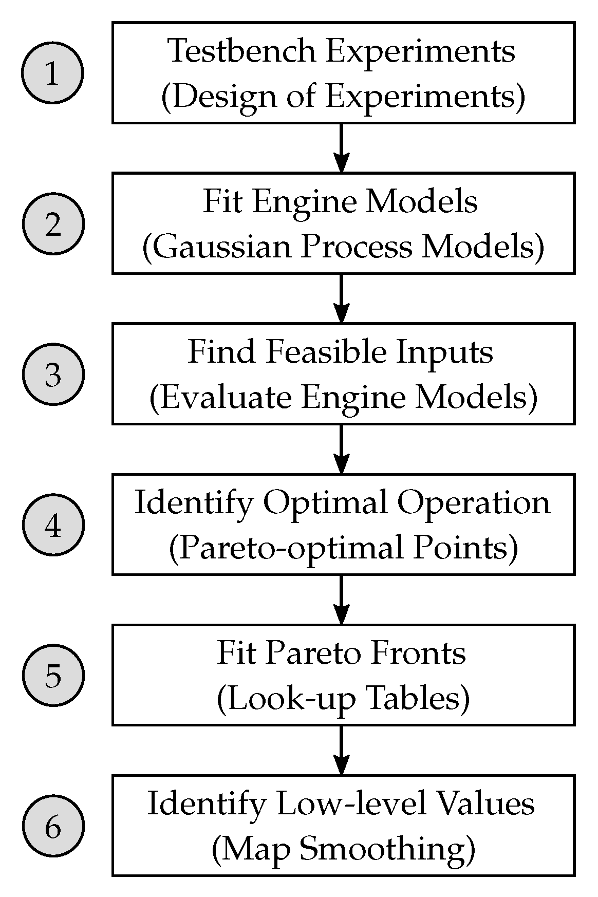
The workflow of the engine preoptimization is shown in Figure 3. The general steps of the procedure are stated in the upper line of each block, while their specific implementation in this work is stated in parentheses underneath. The individual steps are described in the following.

3.1. Testbench Experiments

In order to characterize the engine operation, measurements were taken at a testbench. To fully characterize the engine operation in subsequent steps, it is important that, along with the speed and torque of the engine, all DoF are excited. The excitation must cover the entire range of operation—i.e., not just variations of one input at a time, but a global excitation of all possible combinations.

For this work the measurement campaign was designed using the design of experiments method. A simultaneous variation of the speed, the torque, and all DoF was carried out. Approximately 3000 steady-state measurements were required to accurately train the engine models introduced in the next step. The measurements were taken within approximately one week using an automated testing method, i.e., ORION from A&D Technology.

3.2. Fit Engine Models

Next, engine models were fitted that map the engine speed and torque and the considered engine control inputs to all output variables of interest, i.e., to all output variables relevant to the Pareto optimization, and all output variables that constitute limits to the engine operation.

In this work, Gaussian process (GP) models [28] were trained to map the engine input variables ${\omega }_{\mathrm{e}}$, $T_{\mathrm{e}}$, ${\phi }_{\mathrm{soi}}$, $p_{\mathrm{rail}}$, $u_{\mathrm{vgt}}$, $u_{\mathrm{egr}}$, and $u_{\mathrm{flap}}$ to the output variables. For each output variable an individual GP model was trained. To limit the computational demand of subsequent model evaluations, sparse GP models using pseudo-inputs were trained using the method described in [29]. The procedure to obtain the GP models was:

• Train GP model with an active set size equal to the number of available measurements using Matlab’s machine learning toolbox. The data was scaled to improve the fitting process. The GP models feature a constant basis function and a squared exponential kernel with a separate length scale per predictor.
• Fix the hyperparameters of the GP models to those identified in the previous step. Use the method presented in [29] to identify a number of pseudo-inputs to replace the active set of data points of the previous step. The number of pseudo-inputs required was determined manually for each GP model. As little as 200 pseudo-inputs were sufficient for output variables that are easy to capture, such as the fuel consumption, while up to 2000 pseudo-inputs were required for output variables that are hard to capture, such as the engine-out NO_x emissions.

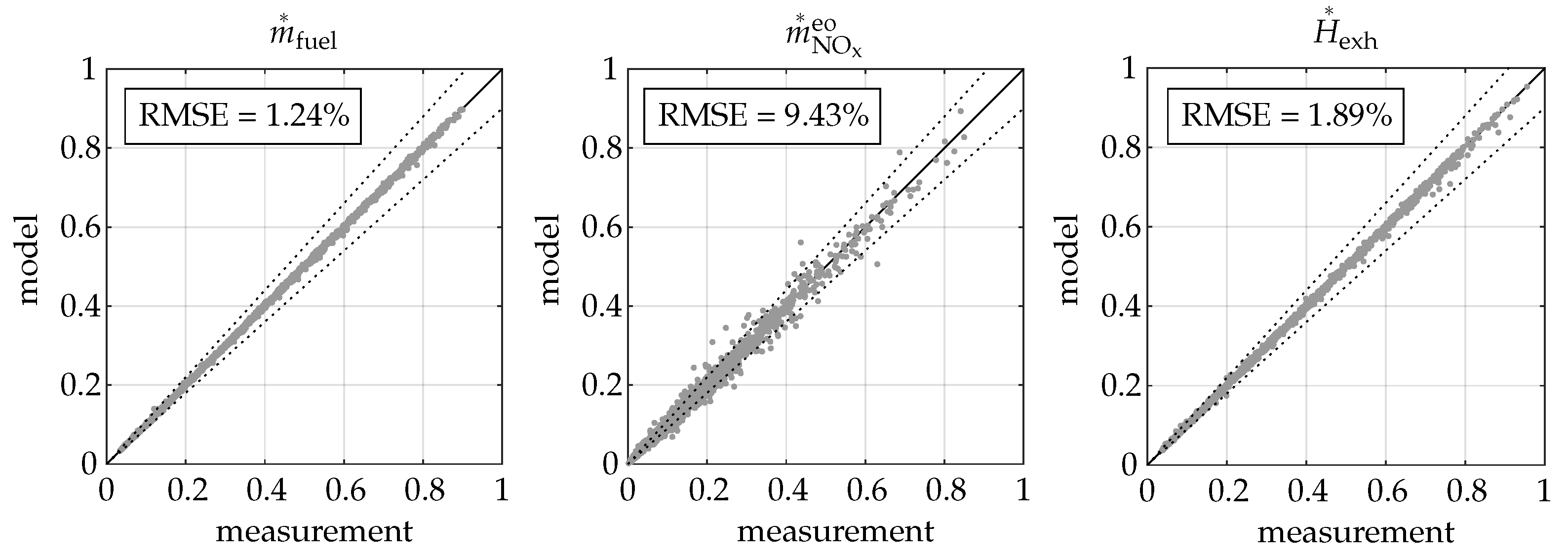
Figure 4 shows the model validation for the fuel mass flow, the engine-out NO_x mass flow, and the exhaust enthalpy ${\stackrel{*}{H}}_{\mathrm{exh}}$ given as

$${\stackrel{*}{H}}_{\mathrm{exh}}={\stackrel{*}{m}}_{\mathrm{exh}}{c}_{\mathrm{p}}{\vartheta }_{\mathrm{exh}}.$$

(10)

Here, ${\stackrel{*}{H}}_{\mathrm{exh}}$ is investigated instead of ${\stackrel{*}{H}}_{\mathrm{ATS}}$, as it does not depend on the ATS temperature. The model outputs are plotted against the respective measured values. The root mean squared error (RMSE) is stated as well. The RMSE of the modeled fuel mass flow and the exhaust enthalpy is approximately 1%. As the NO_x mass flow is harder to model, its RMSE amounts to approximately 10%.

3.3. Find Feasible Inputs

In the first two steps, global measurements and models were considered—i.e., the engine speed and torque were freely variable. In the following, the engine speed and torque as well as the ATS temperature were considered as fixed exogenous inputs and different combinations thereof were considered.

In this third step, the models developed previously were evaluated for all possible engine control input combinations at fixed values of engine speed and torque. The resulting engine operation was checked for feasibility by taking into account a list of operational constraints. The points deemed feasible were stored, while the points deemed infeasible were discarded.

In this work a fine grid of all possible engine control input combinations was built and used to evaluate the GP models developed in the preceding step.

The limits considered include mechanical limits, such as an upper limit on peak cylinder pressure, as well as thermal limits, such as an upper limit on the exhaust temperature, to avoid damage to the engine. Furthermore, drivability limits, such as a lower limit on the torque response, and comfort limits, such as an upper limit on engine noise, were considered to fulfill the driver expectations. Emission-related limits, such as a lower limit on the air-to-fuel ratio, were considered to guarantee a clean combustion.

As the achievable range of operation at very low loads was found to be extremely limited, a fixed operation was used for loads below 10% of the full load.

3.4. Identify Optimal Operation

In this step, the actual preoptimization was performed. Out of all the feasible engine control input combinations identified in the preceding step, the ones that are Pareto-optimal with respect to the multi-objective optimization were identified and stored, while all others were discarded.

In this work, an algorithm is used that identifies and discards dominated points, leaving only non-dominated, i.e., Pareto-optimal, points. It consists of the following three steps:

• A weighted-sum minimization [30] is performed for a grid of objective weights. In this way the points that form a convex lower envelope to the Pareto front are identified.
• The feasible points are sorted. The points identified in the preceding step are placed first, followed by all other points, sorted in ascending order of ${\stackrel{*}{H}}_{\mathrm{ATS}}$.
• Starting at the first point, a point is selected and compared to all other points. Thereby all points dominated by the selected point are discarded. By moving along the remaining points, selecting a point and repeating the comparison above, all dominated points are discarded.

3.5. Fit Pareto Front

In this step, the feasible and Pareto-optimal engine input combinations identified in the two preceding steps were used to parameterize a model of the Pareto front.

In this work, look-up tables were used to characterize the Pareto front. A two-dimensional look-up table was fitted to the previously identified points for each combination of fixed speed, torque, and ATS temperature. This procedure is outlined in the following and was repeated for all points on a grid of speed, torque, and ATS temperature.

To make the interpolation more robust, two transformations are applied before fitting the look-up tables. First, the physical values describing the Pareto front are scaled using their respective minimum and maximum values at the current speed, torque, and ATS temperature. The scaled variables are denoted $J_{\mathrm{X}}$ and are given by

$$\begin{array}{cc}\hfill J_{\mathrm{Hd}}& =\frac{{\stackrel{*}{H}}_{\mathrm{ATS}}-{\stackrel{*}{H}}_{\mathrm{ATS}},\min }{{\stackrel{*}{H}}_{\mathrm{ATS}},\max -{\stackrel{*}{H}}_{\mathrm{ATS}},\min }\hfill \end{array}$$

(11)

$$\begin{array}{cc}\hfill J_{{\mathrm{NO}}_{\mathrm{x}}}& =\frac{{\stackrel{*}{m}}_{{\mathrm{NO}}_{\mathrm{x}}}^{\mathrm{eo}}-{\stackrel{*}{m}}_{{\mathrm{NO}}_{\mathrm{x}},\min }^{\mathrm{eo}}}{{\stackrel{*}{m}}_{{\mathrm{NO}}_{\mathrm{x}},\max }^{\mathrm{eo}}-{\stackrel{*}{m}}_{{\mathrm{NO}}_{\mathrm{x}},\min }^{\mathrm{eo}}}\hfill \end{array}$$

(12)

$$\begin{array}{cc}\hfill J_{\mathrm{fuel}}& =\frac{{\stackrel{*}{m}}_{\mathrm{fuel}}-{\stackrel{*}{m}}_{\mathrm{fuel},\min }}{{\stackrel{*}{m}}_{\mathrm{fuel},\max }-{\stackrel{*}{m}}_{\mathrm{fuel},\min }}.\hfill \end{array}$$

(13)

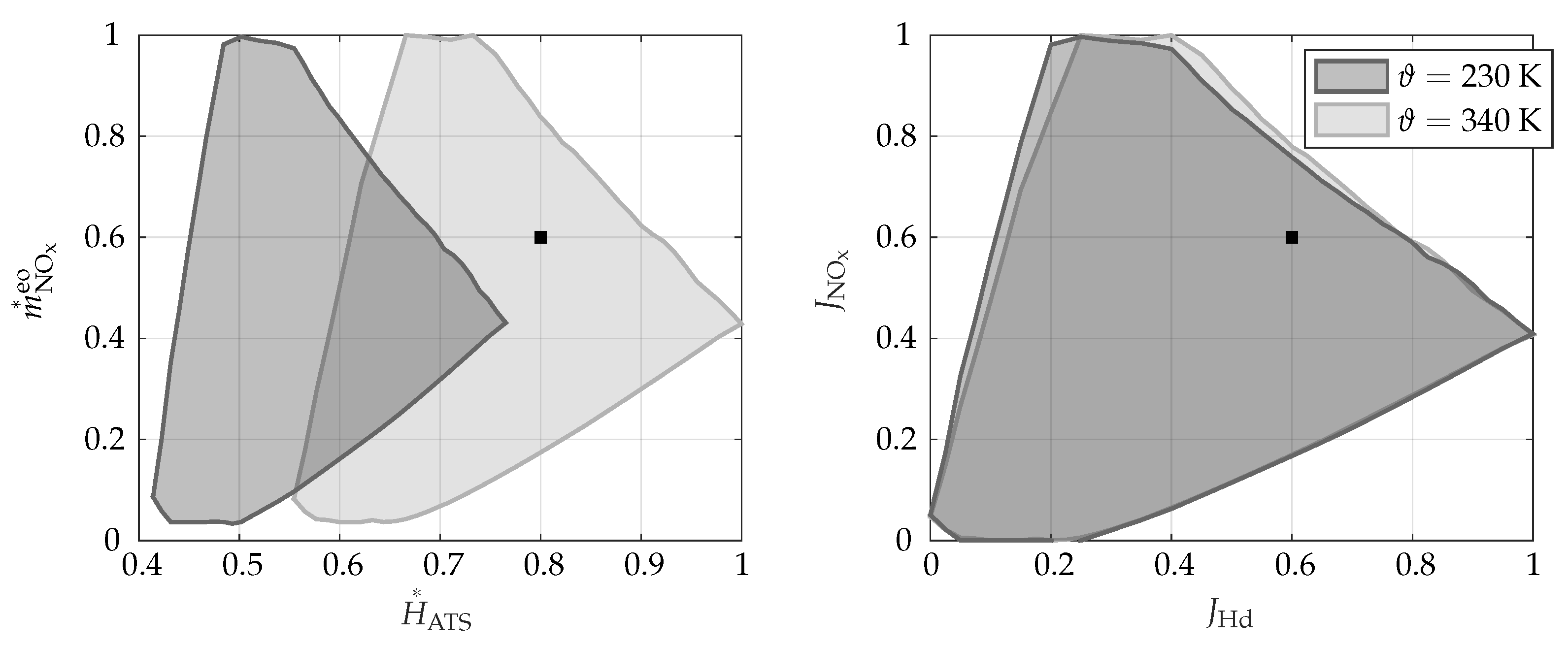
The benefit of this scaling is demonstrated using the example shown in Figure 5. According to Equation (7) the enthalpy provided to the ATS depends on the ATS temperature. As a result, the outline of the Pareto front for a fixed engine speed and torque depends on the ATS temperature, as can be seen in the plot on the left. In this example $\vartheta =230\mathsf{K}$ and $\vartheta =340\mathsf{K}$ are two adjacent ATS temperature grid points and the goal is to evaluate the map at the point represented by the square marker and $\vartheta =285\mathsf{K}$. For the plot on the left, the marked point is not contained in the Pareto front for $\vartheta =340\mathsf{K}$ and the interpolation fails. An ATS temperature dependent scaling results in the plot on the right and avoids this issue. A similar argument can be made for the engine speed and the engine torque.

Second, the Pareto front is rotated by 45${}^{\circ }$ around the $J_{\mathrm{Hd}}$ axis. The scaled and rotated variables are denoted $J_{\mathrm{X}}^{\mathrm{rot}}$ and are given by

$$\begin{array}{cc}\hfill J_{\mathrm{Hd}}^{\mathrm{rot}}& =J_{\mathrm{Hd}}\hfill \end{array}$$

(14)

$$\begin{array}{cc}\hfill J_{{\mathrm{NO}}_{\mathrm{x}}}^{\mathrm{rot}}& =\frac{1}{\sqrt{2}}{J}_{{\mathrm{NO}}_{\mathrm{x}}}-\frac{1}{\sqrt{2}}{J}_{\mathrm{fuel}}\hfill \end{array}$$

(15)

$$\begin{array}{cc}\hfill J_{\mathrm{fuel}}^{\mathrm{rot}}& =\frac{1}{\sqrt{2}}{J}_{{\mathrm{NO}}_{\mathrm{x}}}+\frac{1}{\sqrt{2}}{J}_{\mathrm{fuel}}.\hfill \end{array}$$

(16)

The benefit of this rotation results from the unique form of the Pareto front and the desire to use equally spaced grid points to describe the look-up tables. In the low NO_x region, the fuel consumption rises steeply for a reduction in NO_x emission. Hence, unless a very fine grid is used, a significant interpolation error will result in this region. This problem can be alleviated by rotating the Pareto front around the $J_{\mathrm{Hd}}$ axis. The resulting Pareto front no longer has steep gradients and can be fitted using a coarser grid.

After transferring the identified Pareto-optimal points to scaled and rotated variables, a fuel-cost look-up table $J_{\mathrm{fuel}}^{\mathrm{rot}}(J_{\mathrm{Hd}}^{\mathrm{rot}},J_{{\mathrm{NO}}_{\mathrm{x}}}^{\mathrm{rot}})$, as well as lower and upper bounds for $J_{{\mathrm{NO}}_{\mathrm{x}}}^{\mathrm{rot}}$, were fitted.

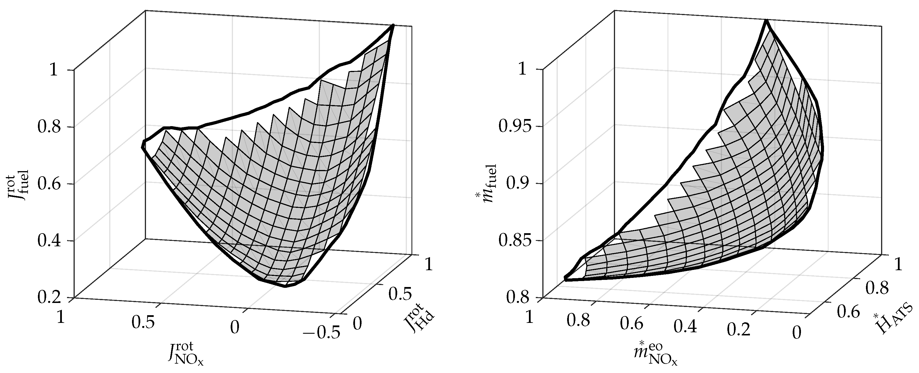
The resulting Pareto front is shown in Figure 6. On the left, the Pareto front fitted to the rotated and scaled values is shown. The gray surface shows the identified Pareto front, while the solid black lines show the $J_{{\mathrm{NO}}_{\mathrm{x}}}^{\mathrm{rot}}$ bounds. On the right, the corresponding Pareto front transferred back to physically meaningful values is shown.

The final result of the preoptimization consists of the following look-up elements. Their relation to Figure 6 is also stated.

• $J_{\mathrm{fuel}}^{\mathrm{rot}}$ with inputs (${\omega }_{\mathrm{e}}$, $T_{\mathrm{e}}$, $\vartheta$, $J_{\mathrm{Hd}}^{\mathrm{rot}}$, $J_{{\mathrm{NO}}_{\mathrm{x}}}^{\mathrm{rot}}$)—gray surface in the plot on the left
• $J_{{\mathrm{NO}}_{\mathrm{x}},\min }^{\mathrm{rot}}$ and $J_{{\mathrm{NO}}_{\mathrm{x}},\max }^{\mathrm{rot}}$ with inputs (${\omega }_{\mathrm{e}}$, $T_{\mathrm{e}}$, $\vartheta$, $J_{\mathrm{Hd}}^{\mathrm{rot}}$)—solid black lines in the plot on the left
• ${\stackrel{*}{H}}_{\mathrm{ATS},\min }$, ${\stackrel{*}{H}}_{\mathrm{ATS},\max }$, ${\stackrel{*}{m}}_{{\mathrm{NO}}_{\mathrm{x}},\min }^{\mathrm{eo}}$, ${\stackrel{*}{m}}_{{\mathrm{NO}}_{\mathrm{x}},\max }^{\mathrm{eo}}$, ${\stackrel{*}{m}}_{\mathrm{fuel},\min }$, and ${\stackrel{*}{m}}_{\mathrm{fuel},\max }$ with inputs (${\omega }_{\mathrm{e}}$, $T_{\mathrm{e}}$, $\vartheta$)—required to map the plot on the left to the one on the right according to Equations (11) to (16)

The preoptimization presented here yields an order reduction of the online optimization performed by the supervisory controller. Instead of having to optimize the five engine control inputs (${\phi }_{\mathrm{soi}}$, $p_{\mathrm{rail}}$, $u_{\mathrm{vgt}}$, $u_{\mathrm{egr}}$, $u_{\mathrm{flap}}$), it is sufficient to optimize the two engine strategy inputs ($J_{\mathrm{Hd}}^{\mathrm{rot}}$, $J_{{\mathrm{NO}}_{\mathrm{x}}}^{\mathrm{rot}}$). Further, the engine limits are fulfilled by design and do not need to be checked during online optimization.

3.6. Identify Low-Level Values

While the preoptimization developed in the preceding steps captures the Pareto-optimal engine operation, it does not return the corresponding engine control inputs, which are required to operate the engine, or the exhaust mass flow, which is required to evaluate the ATS model according to Equation (9).

In this step, an inverse mapping is developed that returns the engine control inputs as a function of the selected Pareto-optimal operation. A similar mapping for the exhaust mass flow is obtained by evaluating the GP models at the engine control inputs obtained by the inverse mapping. Unfortunately, due to the order reduction resulting from the preoptimization, obtaining this inverse mapping is not trivial.

In this work, look-up tables mapping the Pareto-optimal operation, given by (${\omega }_{\mathrm{e}}$, $T_{\mathrm{e}}$, $\vartheta$, $J_{\mathrm{Hd}}^{\mathrm{rot}}$, $J_{{\mathrm{NO}}_{\mathrm{x}}}^{\mathrm{rot}}$), to the engine control inputs ${\phi }_{\mathrm{soi}}$, $p_{\mathrm{rail}}$, $u_{\mathrm{vgt}}$, $u_{\mathrm{egr}}$, and $u_{\mathrm{flap}}$ are used.

These look-up tables were obtained according to the procedure presented in [31]. Thereby an optimization problem was solved that finds a trade-off between how close the resulting engine operation is to the Pareto front and the smoothness of the engine control input look-up tables. In [31], a penalty on the deviation of the inputs from those on the Pareto front was used in the objective, whereas in this work the deviation of the outputs from those on the Pareto front was penalized. This has the advantage that, if the outputs are insensitive to a certain input, this input is smoothed considerably without any deterioration of the overall performance.

A look-up table for the exhaust mass flow was developed by evaluating the GP model for the exhaust mass flow at the grid points of the engine control input look-up tables. It returns ${\stackrel{*}{m}}_{\mathrm{exh}}$ for the inputs (${\omega }_{\mathrm{e}}$, $T_{\mathrm{e}}$, $\vartheta$, $J_{\mathrm{Hd}}^{\mathrm{rot}}$, $J_{{\mathrm{NO}}_{\mathrm{x}}}^{\mathrm{rot}}$).

3.7. Model Validation

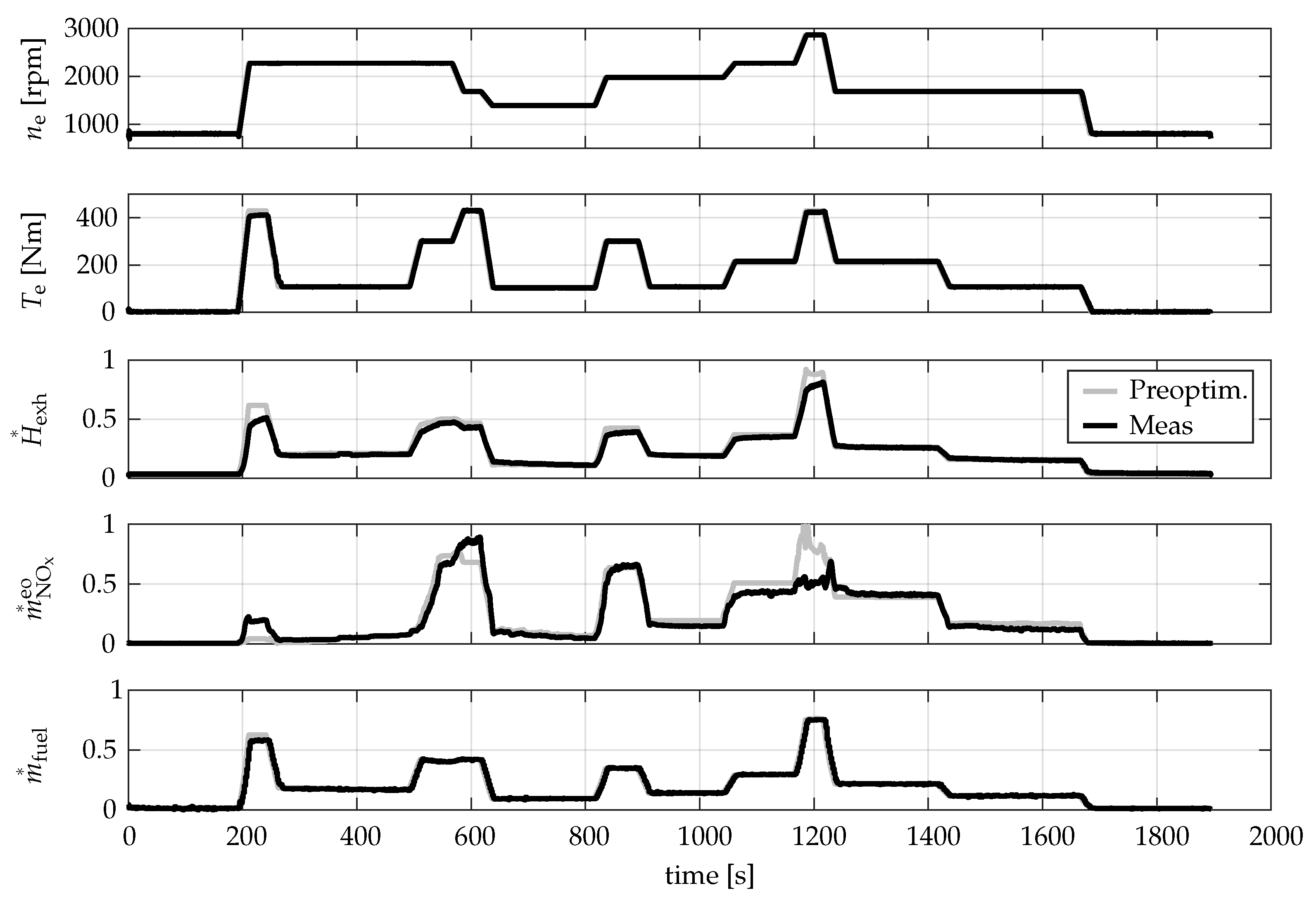
Figure 7 shows the engine operation obtained from the preoptimization, represented by the gray lines, compared to the operation measured at the testbench, represented by the black lines, for the world harmonized stationary cycle (WHSC).

The first plot shows the engine speed, which is controlled by the dynamometer. The second plot shows the torque delivered by the engine. At around 220 s the engine is operated at full load and the requested torque at which the preoptimization is evaluated cannot be reached at the testbench. The fuel mass flow, shown in the bottom plot, shows that insufficient fuel can be injected. This effect is also observed when the original fixed engine calibration is used. Therefore, it should not be attributed to the preoptimization. Throughout the rest of the cycle the requested torque is tracked closely, which shows that the torque response of the engine is not impaired by the preoptimization.

The bottom three plots show the outputs from the Pareto front. To exclude the effect of model mismatch in the thermal model of the ATS, ${\stackrel{*}{H}}_{\mathrm{exh}}$ is shown instead of ${\stackrel{*}{H}}_{\mathrm{ATS}}$. All three variables of interest showed reasonable performance at intermediate loads, i.e., at $T_{\mathrm{e}}\le 350\mathrm{Nm}$. The match in the fuel consumption was good even at full load, i.e., at $T_{\mathrm{e}}=430\mathrm{Nm}$. The match of the NO_x emissions at full load is not as good. This can be attributed to a performance loss in the GP models used for the Pareto preoptimization near the bound of the considered region of operation.

Due to the thermal inertia of the exhaust, the exhaust enthalpy shows a significant dynamic behavior at load steps towards full load. The quasi-static model outputs are not reached in the short duration of the operation at full load. During prolonged full-load operation, however, the exhaust enthalpy converges to the quasi-static value. This means that, while all other dynamics are fast enough to be represented well by the quasi-static engine preoptimization, the thermal exhaust dynamic cannot be captured fully. Nevertheless, the preoptimization represents the actual system sufficiently well to be used for optimization purposes.

4. Optimal Control

In this section, the OCP is formulated based on the vehicle model and the engine preoptimization described in the preceding sections. Dynamic programming is then used to solve the OCP for various powertrain configurations and driving missions.

4.1. Optimal Control Problem

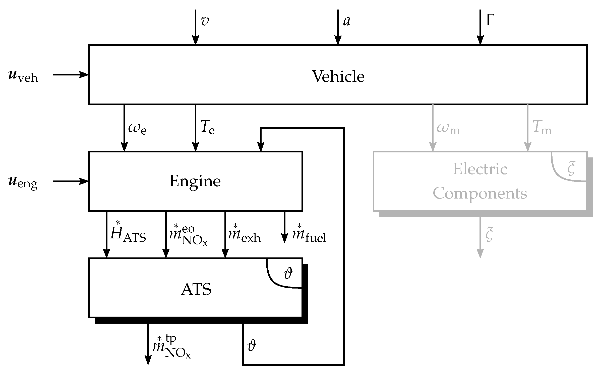
The signal flows within the powertrain model are shown in Figure 8. The speed v, acceleration a, and road gradient $\mathsf{\Gamma }$ are exogenous inputs. Their values are given and cannot be adapted by the supervisory controller.

The vector of vehicle inputs $u_{\mathrm{veh}}$ contains the torque split u, the gear selection i, and the engine on/off decision b.

$$u_{\mathrm{veh}}={\left[uib\right]}^{⊺}$$

(17)

These can be set by the supervisory controller. According to the mission and the selected vehicle inputs, the motor operation is set and the battery state of charge $\xi$ evolves accordingly. The feasible ranges of the vehicle inputs are

$$\begin{array}{cc}\hfill u& \in [-2,2]\hfill \end{array}$$

(18)

$$\begin{array}{cc}\hfill i& \in \{1,2,3,4,5,6\}\hfill \end{array}$$

(19)

$$\begin{array}{cc}\hfill b& \in \{0,1\}.\hfill \end{array}$$

(20)

In theory, no bounds on u are required, as any torque split is feasible as long as all component constraints are met. However, adding a constraint on u allows a finer discretization for the DP optimization which will be presented in the following. The input b describes the engine operation, where at $b=0$ the engine is off and at $b=1$ it is on.

The vector of engine inputs $u_{\mathrm{eng}}$ contains the engine strategy inputs introduced in the preceding section.

$$u_{\mathrm{eng}}={\left[J_{\mathrm{Hd}}^{\mathrm{rot}}{J}_{{\mathrm{NO}}_{\mathrm{x}}}^{\mathrm{rot}}\right]}^{⊺}$$

(21)

The engine speed and torque together with the selected engine strategy inputs, set the engine operation and result in a certain fuel mass flow ${\stackrel{*}{m}}_{\mathrm{fuel}}$, enthalpy flow to the ATS ${\stackrel{*}{H}}_{\mathrm{ATS}}$, engine-out NO_x mass flow ${\stackrel{*}{m}}_{{\mathrm{NO}}_{\mathrm{x}}}^{\mathrm{eo}}$, and exhaust mass flow ${\stackrel{*}{m}}_{\mathrm{exh}}$. As a result of the scaling and the rotation, the feasible engine strategy inputs are

$$\begin{array}{cc}\hfill J_{\mathrm{Hd}}^{\mathrm{rot}}& \in [0,1]\hfill \end{array}$$

(22)

$$\begin{array}{cc}\hfill J_{{\mathrm{NO}}_{\mathrm{x}}}^{\mathrm{rot}}& \in \left[-\frac{1}{\sqrt{2}},\frac{1}{\sqrt{2}}\right].\hfill \end{array}$$

(23)

The NO_x strategy input is further constrained to limit the operation to the achievable range of the preoptimization:

$$J_{{\mathrm{NO}}_{\mathrm{x}}}^{\mathrm{rot}}\in [J_{{\mathrm{NO}}_{\mathrm{x}},\min }^{\mathrm{rot}},J_{{\mathrm{NO}}_{\mathrm{x}},\max }^{\mathrm{rot}}].$$

(24)

The arguments of the $J_{{\mathrm{NO}}_{\mathrm{x}}}^{\mathrm{rot}}$ limits are omitted for reasons of readability.

In Figure 8, the ATS temperature $\vartheta$ is fed back to the engine block, as it influences the enthalpy flow to the ATS, see Equation (7).

The goal of this work is to investigate the trade-off between fuel consumption and tailpipe NO_x emissions. Hence, as in [32], the objective of the OCP is formulated as a weighted sum between the fuel consumption and the tailpipe NO_x emissions, using the NO_x optimization weight $\mu$. Solving the OCP for different values of $\mu$ and plotting the results, yields the trade-off between fuel consumption and NO_x emissions for the considered driving mission. Solving the optimization for a specific NO_x target is equivalent to finding the optimization weight $\mu$ that results in the maximum allowable NO_x emission.

The resulting OCP is

$$\{\begin{array}{c}\hspace{1em} \underset{{\mathbf{u}}_{\mathrm{veh}},{\mathbf{u}}_{\mathrm{eng}}}{\mathrm{minimize}}{\int }_0^{t_{\mathrm{f}}}(1-\mu ){\stackrel{*}{m}}_{\mathrm{fuel}}+\mu {\stackrel{*}{m}}_{{\mathrm{NO}}_{\mathrm{x}}}^{\mathrm{tp}}\mathrm{dt}\hfill \\ \hspace{1em} \mathrm{subject} \mathrm{to} \dot{\xi }=-\frac{I_{\mathrm{b}}}{Q_{\max }\left(\xi \right)}\hfill \\ \hspace{1em}\hspace{1em}\hspace{1em}\hspace{1em}\hspace{1em}\hspace{1em}\dot{\vartheta }=\frac{{\stackrel{*}{H}}_{\mathrm{ATS}}-{\stackrel{*}{Q}}_{\mathrm{hl}}}{C_{\mathrm{ATS}}}\hfill \\ \hspace{1em}\hspace{1em}\hspace{1em}\hspace{1em}\xi \left(0\right)={\xi }_0\hfill \\ \hspace{1em}\hspace{1em}\hspace{1em}\hspace{1em}\xi \left(t_{\mathrm{f}}\right)\ge {\xi }_0\hfill \\ \hspace{1em}\hspace{1em}\hspace{1em}\hspace{1em}\hspace{1em}\hspace{1em}\xi \in [{\xi }_{\min },{\xi }_{\max }]\hfill \\ \hspace{1em}\hspace{1em}\hspace{1em}\hspace{1em}\vartheta \left(0\right)={\vartheta }_0.\hfill \end{array}$$

(25)

The individual components of the objective were normalized in order to evenly distribute the results on the trade-off curve for a grid of $\mu$ values. In order to improve readability, the driving mission and the intermediate equations of the vehicle model stated in Section 2.1 as well as the input bounds and the objective normalization are not stated explicitly.

4.2. DP Optimization

In this work an adapted version of the DP algorithm presented in [33] is used to solve the OCP (25). To formulate a numerical optimization problem, the dynamics are discretized with a sampling time of 1 s. The inputs i and b are integers, which are discrete by design. The remaining states and inputs are discretized using a number of equally spaced grid points. The selected discretization is stated in

Table 1. State and input discretization for DP.

Variable	Type	Points	Steps
$\xi$	State	51	0.006
$\vartheta$	State	46	10 K
$J_{\mathrm{Hd}}^{\mathrm{rot}}$	Input	21	0.05
$J_{{\mathrm{NO}}_{\mathrm{x}}}^{\mathrm{rot}}$	Input	21	0.071
u	Input	41	0.1

.

To obtain the trade-offs investigated in the following sections, a grid for $\mu$ was considered, starting at 0, i.e., fuel-optimal operation, and increasing in increments of 0.1 up to 1, i.e., NO_x-optimal operation. For each value of $\mu$ the OCP (25) was solved.

4.3. Cases Considered

In the following, a number of powertrain configurations with different feature combinations are considered. The OCP (25) represents the most general case and parts of it can be removed if powertrains with fewer features are considered.

The base powertrain corresponds to a conventional vehicle with fixed engine calibration (FEC) and without gear optimization. As a result, there is no input that can be optimized, and the sole dynamic state is the ATS temperature.

Three features, as well as combinations thereof, are considered. The features are variable engine calibration (VEC), gear optimization, and hybridization.

Table 2. Additional states and inputs for each powertrain feature.

Feature	Inputs	States
VEC	$J_{\mathrm{Hd}}^{\mathrm{rot}}$, $J_{{\mathrm{NO}}_{\mathrm{x}}}^{\mathrm{rot}}$	-
Gear optimization	i, b	-
Hybridization	u	$\xi$

lists the inputs and states introduced by each feature. Note that the inputs and states are additive—i.e., if an HEV with gear optimization is considered, the inputs u, i, and b, and the state $\xi$, must be considered. Taking into account all features results in OCP (25).

5. Results for a Conventional Vehicle

In this section, the DP results for the operation of a conventional vehicle are presented. Three cases with different powertrain features are considered, which are shown in

Table 3. Conventional vehicle cases considered.

Case	VEC	Gear Opt.	HEV
Conv FEC	-	-	-
Conv VEC	✓	-	-
Conv VEC w. gears	✓	✓	-

.

For cases without gear optimization, the gear resulting in the lowest fuel consumption for the vehicle with FEC was selected at each time instance. This results in the fuel-optimal operation for Conv FEC.

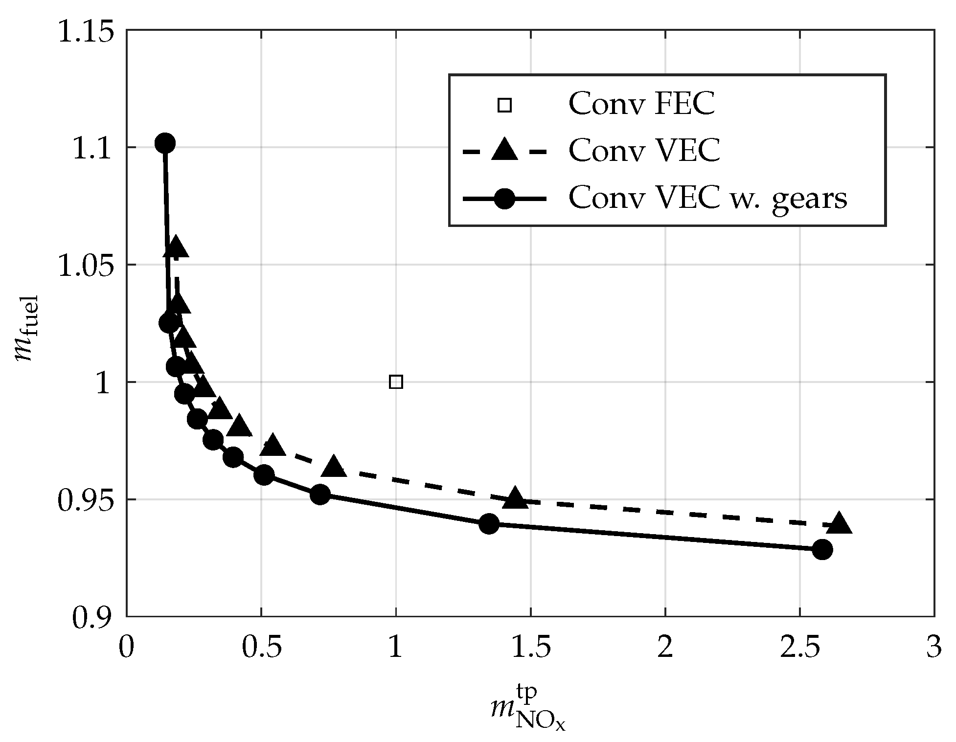
Figure 9 shows the trade-off between fuel consumption and emitted tailpipe NO_x for the three cases on the worldwide harmonized light vehicles test cycle (WLTC) and with an initial ATS temperature below the light-off temperature. For Conv FEC no inputs can be optimized and a fixed operation results, which is represented by the black square. When VEC is introduced, the engine operation can be optimized and the trade-off is shown by the dashed line resulted. When gear optimization is added, the operation of the vehicle can be further optimized and the trade-off shown by the solid line resulted.

Based on these trade-offs, it can be concluded that VEC opens up a considerable range in fuel consumption and tailpipe NO_x emissions through online optimization of the operation to the current mission. By additionally optimizing the gear selection, the trade-off can be improved further. For a fixed NO_x emission limit, compared to Conv FEC, the fuel consumption can be reduced by 4.4% using VEC alone and by 5.4% using VEC and gear optimization. If, on the other hand, the fuel consumption is fixed, the NO_x emissions can be reduced by 73% using VEC alone and by 80% using VEC and gear optimization.

To investigate the origin of this improvement, a simplified driving mission was considered. A constant velocity of 80 km/h and a flat road were assumed for the duration of 1800 s. For the cases without gear optimization, a constant gear was selected throughout the mission, resulting in constant speed and torque of the engine. The initial ATS temperature was set lower than the light-off temperature.

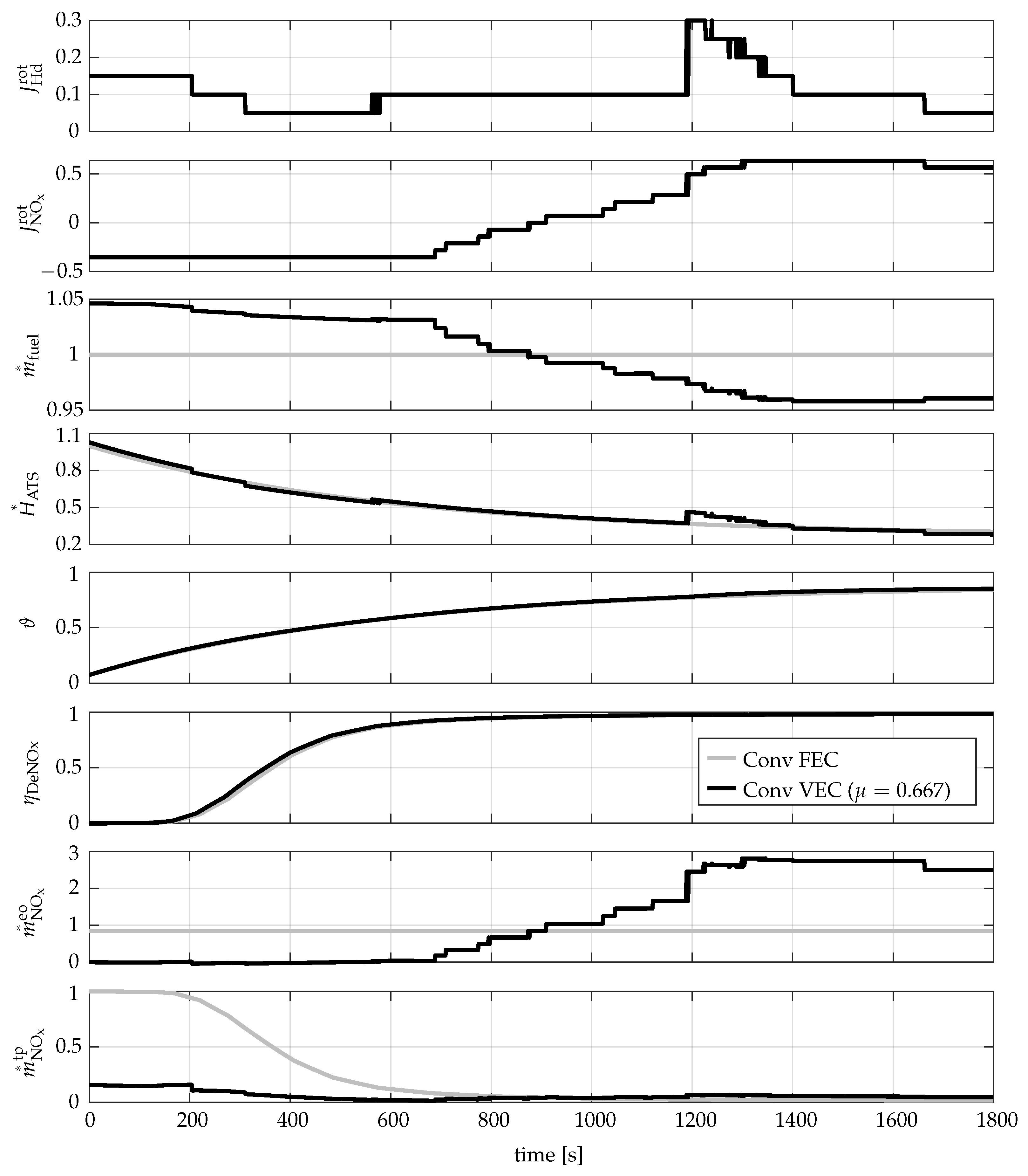
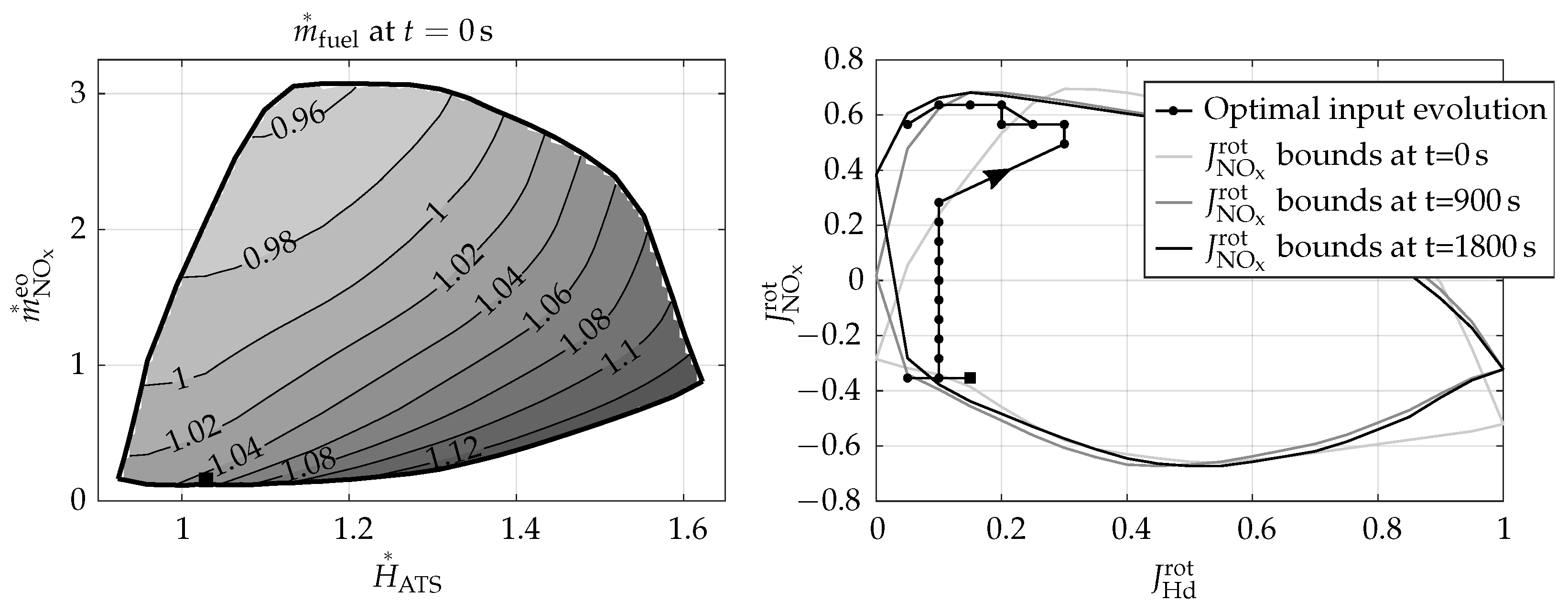
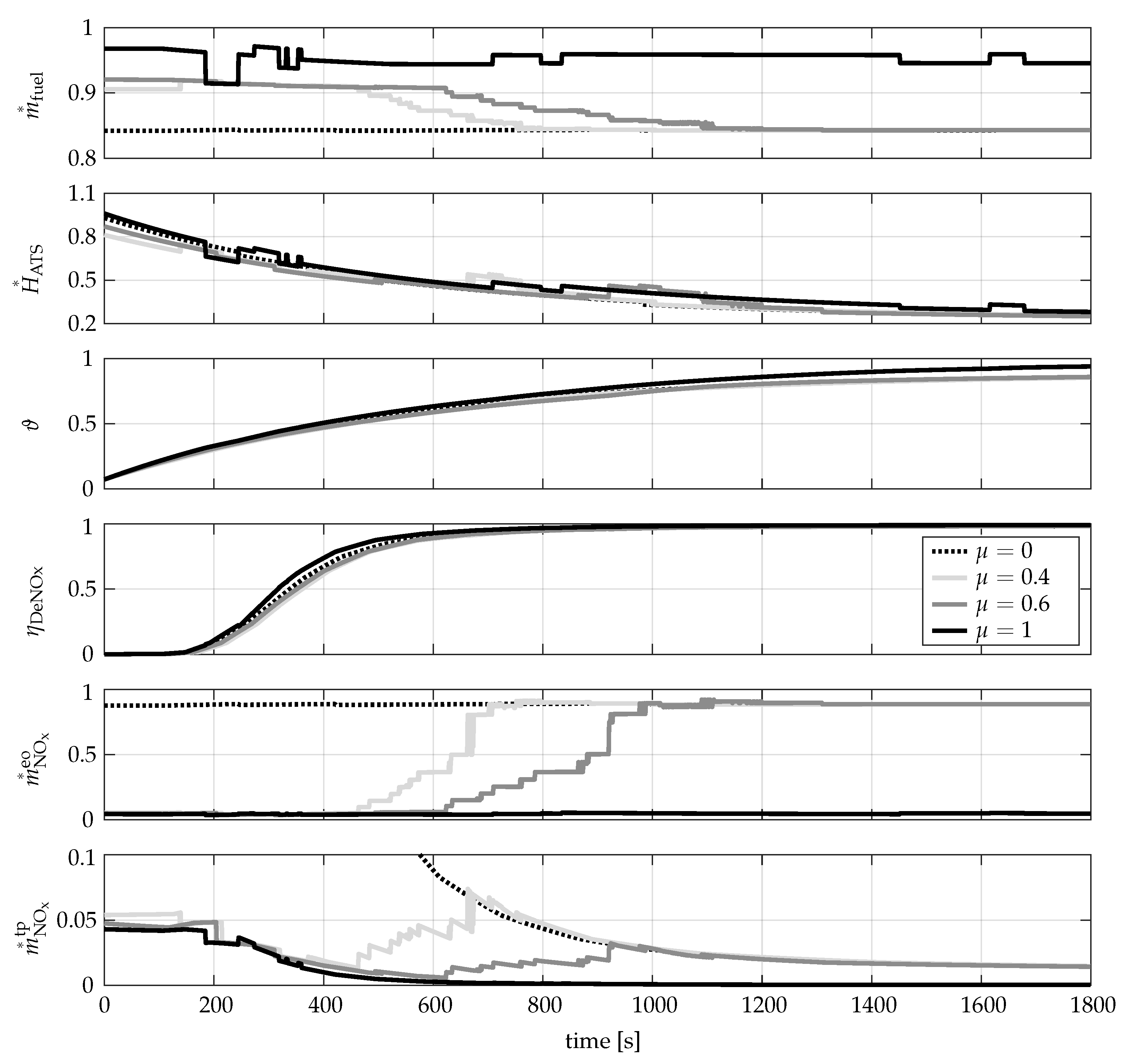
Figure 10 shows the resulting operations for Conv FEC and Conv VEC with equal total fuel consumption ($\mu =0.667$). As the Pareto front depends on the ATS temperature, it changed throughout the cycle, even though the engine speed and torque were constant. The left plot of Figure 11 shows the Pareto front at the initial ATS temperature. The right plot shows the evolution of the optimal engine strategy inputs and $J_{{\mathrm{NO}}_{\mathrm{x}}}^{\mathrm{rot}}$ bounds at different times along the mission.

At the start of the mission, when the ATS was cold and the NO_x-reduction efficiency was low, the engine was operated with minimal engine-out NO_x emissions and high fuel consumption. The resulting operation on the Pareto front is shown by the square in the lower left corner in the left plot of Figure 11. At the end of the mission, the engine was operated with minimal fuel consumption and high engine-out NO_x emissions.

During the mission, the optimal engine operation was selected by carefully balancing the individual objectives of the Pareto front. From the start of the mission to 700 s, the engine-out NO_x emissions were kept to a minimum. The operation was shifted towards the bottom left corner of the Pareto front, which resulted in a gradual decrease in the fuel consumption. From 700 to 1200 s, the engine-out NO_x emissions were increased and the fuel consumption was decreased. The operation was shifted upwards along the left-hand boundary of the Pareto front. As the NO_x-reduction efficiency of the ATS rose, the tailpipe NO_x emissions remained low. At 1200 s, the operation jumped to a higher engine-out NO_x mass flow and a higher enthalpy provided to the ATS at equal fuel consumption. On the Pareto front, this corresponds to a jump along an iso-fuel line. From 1200 to 1400 s, Conv VEC increased the enthalpy provided to the ATS—i.e., active ATS heating occurred. At the end of this active heating phase, the ATS temperature was around 6 ${}^{\circ }$C higher than for Conv FEC. During this active heating phase, the operation was gradually moved to the left of the Pareto front towards the fuel-optimal operation. From 1400 s to the end of the cycle, the engine was operated near the fuel-optimal operation. As the ATS was then fully operational, the engine-out NO_x emissions were successfully reduced, and the tailpipe NO_x emissions remained low.

It is worth pointing out that the active ATS heating phase occurred when the NO_x-reduction efficiency was already high, i.e., above 90%. Actively heating the ATS at very low ATS temperatures does not result in a direct advantage, as the increase in the current NO_x-reduction efficiency is negligible, but it leads to higher heat losses throughout the mission. When the ATS is not operational, instead of actively heating the ATS, the engine-out NO_x emissions should be minimized. Only once the NO_x-reduction efficiency reaches a certain level, is it beneficial to increase the enthalpy provided to the ATS at the cost of an increased fuel consumption and/or engine-out NO_x emissions.

To investigate the differences in operation for different NO_x optimization weights, the optimal solutions for four values of $\mu$ are shown in Figure 12. The dotted line represents the fuel-optimal operation, i.e., $\mu =0$. The three solid lines show the operation for increasing $\mu$.

For $\mu =0$ the fuel-optimal operation was selected throughout the cycle. In the plot of the Pareto front, this corresponds to the top left corner. The resulting constant engine operation led to very high tailpipe NO_x emissions at the beginning of the cycle.

For $\mu =1$, i.e., NO_x-minimal operation, the engine operation was consistently selected in the region with minimal engine-out NO_x emisions, i.e., near the square marker shown in the left plot of Figure 11. Within this region, the operation was chosen as far to the right as possible, without entering the region where increasing the enthalpy provided to the ATS results in an increase in engine-out NO_x emissions. This means that even if the fuel consumption is of no interest, it is not worth increasing the ATS temperature, if this results in an increase of the engine-out NO_x emissions. This is equivalent to stating that the current cost corresponding to an increase in tailpipe NO_x emissions will outweigh any future advantage that can be achieved by actively heating the ATS.

The optimal solutions for $\mu =0.4$ and $\mu =0.6$ underwent the same phases as the solution for $\mu =0.667$, which was analyzed above. However, the duration and the timing of the individual phases differed among the solutions. For $\mu =0.4$ each of the phases—low NO_x, gradual shift to higher NO_x, and active ATS heating—was shorter than its counterpart for $\mu =0.6$. The fuel-optimal operation was reached sooner, resulting in lower overall fuel consumption with higher tailpipe NO_x emissions.

The unsmooth input trajectories observed in the DP optimization results were attributed to the linear interpolation used to evaluate the look-up tables. To achieve smoother input trajectories, a continuously differentiable model of the Pareto front should be developed and used instead of the look-up tables. Only then will a finer discretization of the states and inputs in the DP optimization be advantageous. In this work, the focus was on investigating the potential of vehicles with different powertrain features. As a result, many DP optimizations for different powertrain features and driving missions must carried out, and it is more important to limit the computational demand of these optimizations than to achieve smooth input trajectories.

6. Results for an HEV

In this section, the DP results for the operation of an HEV are presented. In the following, the five cases shown in

Table 4. HEV cases considered.

Case	VEC	Gear Opt.	HEV
Conv FEC	-	-	-
HEV FEC	-	-	✓
HEV FEC w. gears	-	✓	✓
HEV VEC	✓	-	✓
HEV VEC w. gears	✓	✓	✓

are considered.

For the HEV cases without gear optimization, it was assumed that the clutch was engaged whenever the vehicle was moving. This means that while purely electric driving was possible, the engine needed to be motored and added a significant drag. When gear optimization was introduced, it was assumed that the clutch was disengaged during fuel cut-off phases. As a result, the engine could be decoupled rather than motored during purely electric driving.

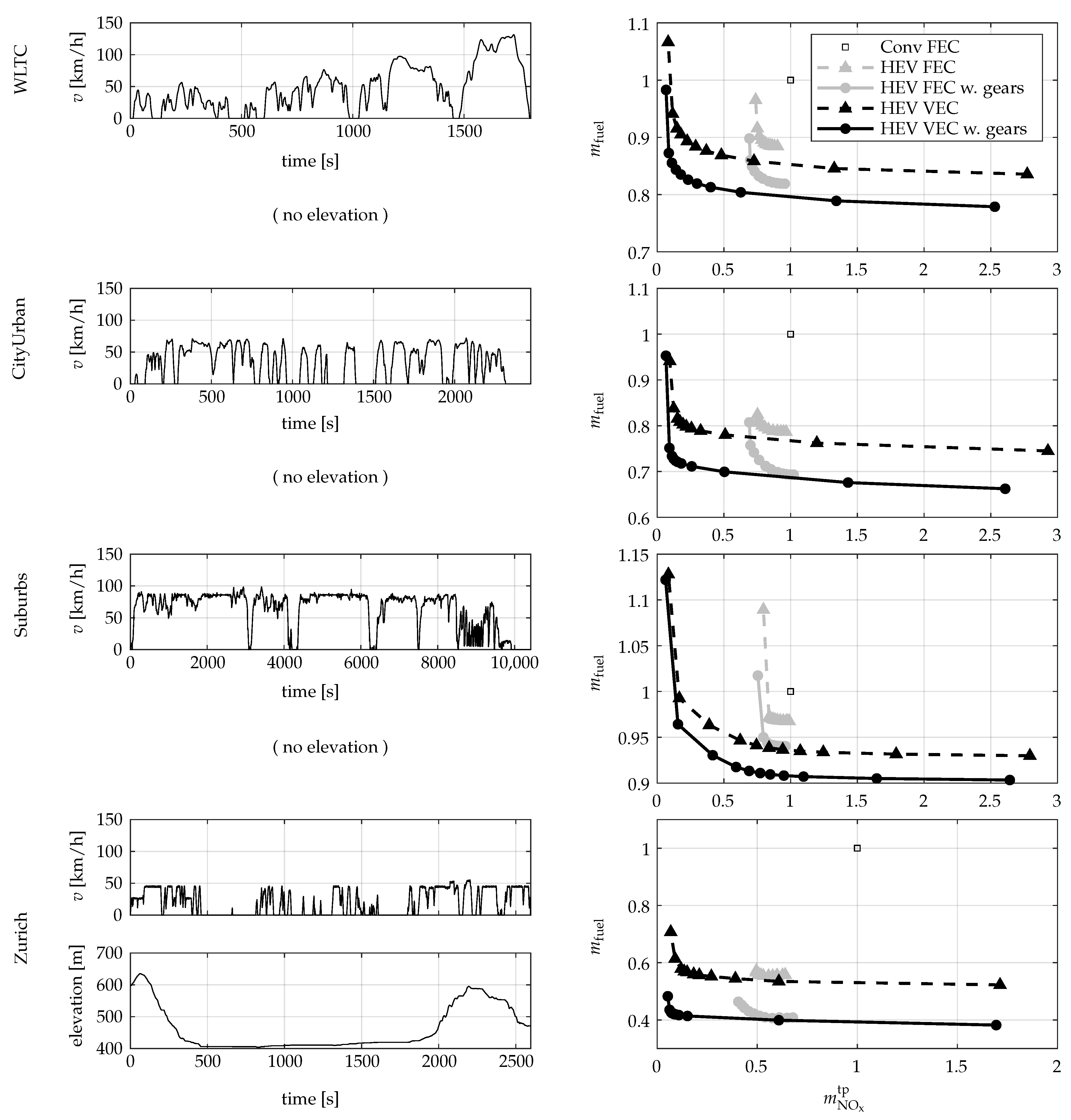
During the investigation, the four driving missions shown in Figure 13 were considered. The plots on the left show the vehicle velocity, and where applicable, the elevation profile for each driving mission. The plots on the right show, the corresponding trade-offs between the fuel consumption and the emitted tailpipe NO_x. First, the WLTC is considered. The second driving mission, denoted CityUrban, was an urban mission obtained with a vehicle comparable to the one considered in this work. The third driving mission, denoted Suburbs, was obtained in the same way, but featured higher velocities and was much longer. The first three driving missions were assumed to feature a flat road. The fourth driving mission, denoted Zurich, was obtained using the method presented in [34] and included a pronounced elevation profile from which the road gradient was calculated.

The potential for fuel consumption reduction through hybridization is strongly dependent on the vehicle mission. Missions with frequent braking phases or pronounced elevation profiles offer ample opportunity for recuperation. As a result, through hybridization alone, the fuel consumption on the WLTC, the CityUrban driving mission, and the Zurich driving mission, could be reduced by roughly 12%, 21%, and 45%, respectively, when the NO_x emission limit was set to that of Conv FEC. For the Suburbs driving mission, which featured prolonged operation at higher velocity and did not offer any significant recuperation phases, the achievable reduction in the fuel consumption was only 3%.

For a constant requested power, the fuel consumption increases with a rising engine speed, while the engine-out NO_x emissions remain approximately constant. As a result, the effect of the gear selection on the fuel consumption was more pronounced than its effect on the NO_x emissions. The achievable advantage through gear optimizing was larger for missions with low and/or frequently changing vehicle velocities. The fuel consumption was also lower, as the gear optimization allowed the engine drag losses to be avoided during fuel cut-off phases by decoupling the engine from the drivetrain.

While optimizing the vehicle inputs enabled a trade-off between fuel consumption and NO_x emission, this region was drastically extended for all missions considered if VEC was enabled. Most notably, the region with very low NO_x emissions could only be reached if the engine operation could also be optimized by the supervisory controller.

In summary, the results show that while hybridization on its own offers the possibility to significantly reduce the fuel consumption, the potential to reduce the vehicle’s tailpipe NO_x emissions is limited. When additionally VEC is enabled, a further, but limited reduction in the fuel consumption is possible, while the tailpipe NO_x emissions can be reduced drastically.

7. Conclusions

In this work, the potential for improving the trade-off between fuel consumption and tailpipe NO_x emissions through variable engine calibration (VEC) was investigated for both conventional and hybrid electric vehicles (HEV). First, a preoptimization procedure was presented that simplifies the powertrain optimization without any loss of performance. Next, dynamic programming (DP) was used to find the optimal fuel versus tailpipe NO_x trade-off curves for different vehicle configurations and driving missions.

The presented engine preoptimization results in an order reduction in the optimal control problem that must be solved by the supervisory controller and guarantees a feasible engine operation. As a result, the powertrain optimization becomes much less computationally demanding.

Simulation results showed that, for a conventional vehicle and the worldwide harmonized light vehicles test cycle (WLTC), the fuel consumption can be reduced by 4.4% at equivalent NO_x emissions when VEC is introduced. If, additionally, the gears are optimized, the fuel consumption can be reduced by a further 1%. At equivalent fuel consumption, the tailpipe NO_x emissions can be reduced by 73% when VEC is introduced, and by a further 7% when the gears are also optimized.

For an HEV without gear optimization and all cycles considered, the achievable trade-off in fuel consumption and tailpipe NO_x emissions was increased considerably through the introduction of VEC in simulation. A similar improvement was obtained for an HEV with gear optimization.

Pollutant emission limits of future emissions legislation are expected to be lowered drastically [35]. As a result, there is a strong need for technological advances that can reduce pollutant emissions, ideally without further increasing powertrain complexity. In this work, it was shown that VEC can be considered a key enabler for meeting strict pollutant legislation, as the powertrain operation can be adapted to the respective driving mission. Thereby the performance of a given powertrain is maximized solely through software.

The proposed engine preoptimization method can easily be applied to a multitude of different engine configurations, as the engine model used by the supervisory controller, i.e., the Pareto front, no longer depends on the specific engine configuration but only on the objectives for which the Pareto front is formed. This simplifies the transferability of the method, as the optimal control problem (OCP) that must be solved is independent of the specific engine configuration. Furthermore, the order reduction of the OCP results in a faster optimization and forms the first step towards online optimization.

Based on the work presented in this publication, there are two avenues for future research. First, the presented method can be used to investigate the potential of powertrain layouts and can help identify an optimal powertrain configuration and component sizing.

Second, the presented methodology can be used as the basis for the development of an online optimal controller. A promising approach is to implement a model predictive control algorithm that optimizes the operation of the powertrain for a predicted driving mission online. By reoptimizing the vehicle operation periodically, the algorithm can account for mispredictions of the driving mission and model mismatches.

References

1. EU Emission Standards—Cars and Light Trucks. Available online: https://dieselnet.com/standards/eu/ld.php (accessed on 3 November 2021).
2. Guzzella, L.; Onder, C. Introduction to Modeling and Control of Internal Combustion Engine Systems; Springer Science & Business Media: Berlin/Heidelberg, Germany, 2009. [Google Scholar]
3. Regulation (EU) 2019/631 of the European Parliament an the Council—Setting CO2 Emission Performance for New Passenger Cars and for Light Commercial Vehicles. Available online: https://eur-lex.europa.eu/legal-content/EN/TXT/PDF/?uri=CELEX:02019R0631-20210301&from=EN (accessed on 3 November 2021).
4. ACEA Pocket Guide 2021/2022. Available online: https://www.acea.auto/files/ACEA_Pocket_Guide_2021-2022.pdf (accessed on 3 November 2021).
5. Guzzella, L.; Sciarretta, A. Vehicle Propulsion Systems; Springer: Berlin/Heidelberg, Germany, 2007; Volume 1. [Google Scholar]
6. Sciarretta, A.; Guzzella, L. Control of hybrid electric vehicles. IEEE Control. Syst. Mag. 2007, 27, 60–70. [Google Scholar]
7. Zentner, S.; Asprion, J.; Onder, C.; Guzzella, L. An equivalent emission minimization strategy for causal optimal control of Diesel engines. Energies 2014, 7, 1230–1250. [Google Scholar] [CrossRef] [Green Version]
8. Nüesch, T.; Cerofolini, A.; Mancini, G.; Cavina, N.; Onder, C.; Guzzella, L. Equivalent consumption minimization strategy for the control of real driving NOx emissions of a Diesel hybrid electric vehicle. Energies 2014, 7, 3148–3178. [Google Scholar] [CrossRef] [Green Version]
9. Kessels, J.; Willems, F.; Schoot, W.; Van Den Bosch, P. Integrated energy & emission management for hybrid electric truck with SCR aftertreatment. In Proceedings of the 2010 IEEE Vehicle Power and Propulsion Conference (VPPC), Lille, France, 1–3 September 2010; pp. 1–6. [Google Scholar]
10. Cloudt, R.; Willems, F. Integrated Emission Management strategy for cost-optimal engine-aftertreatment operation. SAE Int. J. Engines 2011, 4, 1784–1797. [Google Scholar] [CrossRef]
11. Donkers, M.; Van Schijndel, J.; Heemels, W.; Willems, F. Optimal control for integrated emission management in Diesel engines. Control. Eng. Pract. 2017, 61, 206–216. [Google Scholar] [CrossRef] [Green Version]
12. Karim, M.R.; Egardt, B.; Murgovski, N.; Gelso, E.R. Supervisory control for real-driving emission compliance of heavy-duty vehicles. IFAC-PapersOnLine 2018, 51, 460–466. [Google Scholar] [CrossRef]
13. Geiselhart, R.; Bergmann, D.; Niemeyer, J.; Remele, J.; Graichen, K. Hierarchical optimization of operational costs of a heavy-duty Diesel engine and an exhaust aftertreatment system. In Proceedings of the 2019 18th European Control Conference (ECC), Naples, Italy, 25–28 June 2019; pp. 1227–1232. [Google Scholar]
14. Van Dooren, S.; Balerna, C.; Salazar, M.; Amstutz, A.; Onder, C.H. Optimal Diesel engine calibration using convex modelling of Pareto frontiers. Control. Eng. Pract. 2020, 96, 104313. [Google Scholar] [CrossRef]
15. Guardiola, C.; Pla, B.; Bares, P.; Waschl, H. Adaptive calibration for reduced fuel consumption and emissions. Proc. Inst. Mech. Eng. Part D J. Automob. Eng. 2016, 230, 2002–2014. [Google Scholar] [CrossRef]
16. Elbert, P.; Amstutz, A.; Onder, C. Adaptive control for the real driving emissions of Diesel engines. MTZ Worldw. 2017, 78, 68–74. [Google Scholar] [CrossRef]
17. Tschopp, F.; Nüesch, T.; Wang, M.; Onder, C. Optimal Energy and Emission Management of a Diesel Hybrid Electric Vehicle Equipped with a Selective Catalytic Reduction System; Technical Report, SAE Technical Paper; SAE: Warrendale, PA, USA, 2015. [Google Scholar]
18. Simon, A.; Nelson-Gruel, D.; Charlet, A.; Jaine, T.; Nouillant, C.; Chamaillard, Y. Optimal supervisory control of a Diesel HEV taking into account both DOC and SCR efficiencies. IFAC-PapersOnLine 2018, 51, 323–328. [Google Scholar] [CrossRef]
19. Ritzmann, J.; Lins, G.; Onder, C. Optimization method for the energy and emissions management of a hybrid electric vehicle with an exhaust aftertreatment system. IFAC-PapersOnLine 2020, 53, 13797–13804. [Google Scholar] [CrossRef]
20. Willems, F.; Spronkmans, S.; Kessels, J. Integrated powertrain control to meet low CO2 emissions for a hybrid distribution truck with SCR-deNOx system. In Proceedings of the ASME 2011 Dynamic Systems and Control Conference and Bath/ASME Symposium on Fluid Power and Motion Control, Arlington, VA, USA, 31 October–2 November 2011; American Society of Mechanical Engineers: New York, NY, USA, 2011; pp. 907–912. [Google Scholar]
21. Maamria, D.; Sciarretta, A.; Chaplais, F.; Petit, N. Online energy management system (EMS) including engine and catalyst temperatures for a parallel HEV. IFAC-PapersOnLine 2017, 50, 8913–8920. [Google Scholar] [CrossRef]
22. Zhao, J.; Wang, J. Model predictive control of integrated hybrid electric powertrains coupled with aftertreatment systems. In Proceedings of the ASME 2014 Dynamic Systems and Control Conference, San Antonio, TX, USA, 22–24 October 2014; American Society of Mechanical Engineers: New York, NY, USA, 2014. [Google Scholar]
23. Ma, Y.; Wang, J. Integrated power management and aftertreatment system control for hybrid electric vehicles with road grade preview. IEEE Trans. Veh. Technol. 2017, 66, 10935–10945. [Google Scholar] [CrossRef]
24. Kuchly, J.; Nelson-Gruel, D.; Charlet, A.; Chamaillard, Y.; Nouillant, C. Projected gradient and model predictive control: Optimal energy and pollutants management for hybrid electric vehicle. IFAC-PapersOnLine 2019, 52, 121–127. [Google Scholar] [CrossRef]
25. Feru, E.; Murgovski, N.; de Jager, B.; Willems, F. Supervisory control of a heavy-duty Diesel engine with an electrified waste heat recovery system. Control Eng. Pract. 2016, 54, 190–201. [Google Scholar] [CrossRef]
26. Ritzmann, J.; Christon, A.; Salazar, M.; Onder, C. Fuel-Optimal Power Split and Gear Selection Strategies for a Hybrid Electric Vehicle; SAE Technical Papers; SAE International: Warrendale, PA, USA, 2019. [Google Scholar] [CrossRef]
27. Marler, R.T.; Arora, J.S. Survey of multi-objective optimization methods for engineering. Struct. Multidiscip. Optim. 2004, 26, 369–395. [Google Scholar] [CrossRef]
28. Rasmussen, C.E.; Williams, C.K. Gaussian Processes for Machine Learning; MIT Press: Cambridge, MA, USA, 2006; p. 272. [Google Scholar]
29. Snelson, E.; Ghahramani, Z. Sparse Gaussian processes using pseudo-inputs. In Advances in Neural Information Processing Systems; Citeseer: San Jose, CA, USA, 2006; pp. 1257–1264. [Google Scholar]
30. Marler, R.T.; Arora, J.S. The weighted sum method for multi-objective optimization: New insights. Struct. Multidiscip. Optim. 2010, 41, 853–862. [Google Scholar] [CrossRef]
31. Pandey, V.; van Dooren, S.; Ritzmann, J.; Pla, B.; Onder, C. Variable smoothing of optimal Diesel engine calibration for improved performance and drivability during transient operation. Int. J. Engine Res. 2020, 22, 1888–1895. [Google Scholar] [CrossRef]
32. Nüesch, T.; Wang, M.; Voser, C.; Guzzella, L. Optimal energy management and sizing for hybrid electric vehicles considering transient emissions. IFAC Proc. Vol. 2012, 45, 278–285. [Google Scholar] [CrossRef]
33. Sundström, O.; Guzzella, L. A generic dynamic programming Matlab function. In Proceedings of the 2009 IEEE Control Applications, (CCA) & Intelligent Control, (ISIC), St. Petersburg, Russia, 8–10 July 2009; pp. 1625–1630. [Google Scholar]
34. Behrisch, M.; Bieker, L.; Erdmann, J.; Krajzewicz, D. SUMO–simulation of urban mobility: An overview. In Proceedings of the SIMUL 2011, The Third International Conference on Advances in System Simulation, Barcelona, Spain, 23–28 October 2011. [Google Scholar]
35. Scenarios for HDVs: Summary emission limits and test conditions. Available online: https://circabc.europa.eu/sd/a/b706ffba-f863-4d23-809d-20d9f18ecba4/AGVE (accessed on 17 September 2021).
Figure 1. Vehicle powertrain layout. The components shown in gray are featured in the HEV, but not in the conventional vehicle.
Energies 14 07606 g001
Figure 2. Pareto fronts showing the trade-off between fuel consumption and engine-out NOx emissions for different sets of DoF at fixed engine speed and torque. All values were normalized.
Energies 14 07606 g002
Figure 3. Workflow of the engine preoptimization. The general steps of the procedure are stated in the upper line of each block, while their specific implementation in this work is stated in parentheses underneath.
Energies 14 07606 g003
Figure 4. Validation of the GP models. The plots show the modeled values versus the measured values for the individual engine objectives. Each solid black line shows a perfect match, and the dotted lines show regions with ±10% error.
Energies 14 07606 g004
Figure 5. Outline of the Pareto front for fixed engine speed and torque and two values of the ATS temperature. The plot on the right shows values normalized using a constant value. The plot on the left shows values scaled using Equations (11) and (12). The square marker represents an exemplary evaluation point.
Energies 14 07606 g005
Figure 6. Exemplary Pareto front at an engine speed of 2000 rpm, an engine torque of 200 Nm, and an ATS temperature of 340 K. The image on the left shows the fitted Pareto front described by scaled and rotated values. The image on the right shows the fitted Pareto front transferred back to physically meaningful values. The values in the plot on the right were normalized.
Energies 14 07606 g006
Figure 7. Model validation on the world harmonized stationary cycle (WHSC). The values in the bottom three plots were normalized.
Energies 14 07606 g007
Figure 8. Signal flows within the powertrain model. The blocks featured only in the HEV are shown in gray.
Energies 14 07606 g008
Figure 9. Trade-off between fuel consumption and emitted tailpipe NOx on the WLTC with an initial ATS temperature below the light-off temperature. The markers represent individual DP optimizations for specific values of μ . All values were normalized.
Energies 14 07606 g009
Figure 10. Comparison of operation with FEC to that with VEC for the simplified driving mission. All values were normalized.
Energies 14 07606 g010
Figure 11. The left plot shows the Pareto front at the initial ATS temperature for the Conv VEC case on the simplified driving mission. The square marker shows the operation selected by the optimization. The right plot shows the evolution of the optimal engine strategy inputs and their bounds. All values were normalized.
Energies 14 07606 g011
Figure 12. Comparison of the operation of the Conv VEC case at different NOx optimization weights μ for the simplified driving mission. All values were normalized.
Energies 14 07606 g012
Figure 13. Optimal operation of an HEV. The driving missions are shown on the left, and the resulting trade-offs between fuel consumption and emitted NOx are shown on the right. An initial ATS temperature below the light-off temperature was used for all driving missions. All values were normalized.
Energies 14 07606 g013