Assessing Maximum Power Point Tracking Intelligent Techniques on a PV System with a Buck–Boost Converter

Abstract

Classic and intelligent techniques aim to locate and track the maximum power point of photovoltaic (PV) systems, such as perturb and observe (P&O), fuzzy logic (FL), artificial neural networks (ANNs), and adaptive neuro-fuzzy inference systems (ANFISs). This paper proposes and compares three intelligent algorithms for maximum power point tracking (MPPT) control, specifically fuzzy, ANN, and ANFIS. The modeling of a single-diode equivalent circuit-based 3 kWp PV plant was developed and validated to achieve this purpose. Then, the MPPT techniques were designed and applied to control the buck–boost converter’s switching device of the PV plant. All three methods use the ambient conditions as input variables: solar irradiance and ambient temperature. The proposed methodology comprises the study of the dynamic response for tracking the maximum power point and the power generated of the PV systems, and it was compared to the classic P&O technique under varying ambient conditions. We observed that the intelligent techniques outperformed the classic P&O method in tracking speed, tracking accuracy, and reducing oscillation around the maximum power point (MPP). The ANN technique was the better control algorithm in energy gain, managing to recover up to 9.9% power.

1. Introduction

The insertion of photovoltaic (PV) systems into the world electrical matrix has grown exponentially. However, the nonlinear nature of PV arrays regarding ambient conditions and unstable climatic factors hinders the extraction of the maximum power provided by the PV modules. As a result, the PV modules can extract a false MPP and convert less solar energy into electrical energy. Consequently, there is a reduction in the efficiency of the PV system [1].

The reduction in the efficiency of PV systems becomes substantial when it comes to photovoltaic plants with a high installed capacity. Therefore, maximum power point tracking (MPPT) techniques that are minimally more efficient than others can increase the generated power significantly. As a result, researchers have studied and developed MPPT techniques extensively.

MPPT is a technique that allows PV arrays to operate at the maximum power production based on a control system. They diverge in aspects such as the number of required sensors, complexity, cost, speed convergence, and accurate tracking under irradiance and/or temperature variations [2].

MPPT techniques are helpful to add speed in the search process for the new MPP when the ambient conditions change and, consequently, the MPP of the module is modified. For example, an inefficient MPPT technique can follow the MPP under normal ambient conditions with little or no damage to the power supplied to the system. However, on the other hand, this same technique may not keep up with the MPP when there are many passing clouds in short time intervals or a false MPP is detected. Unfortunately, this can damage the power generation of the PV system. Therefore, choosing the ideal MPPT technique according to ambient conditions is important to extract the maximum power generation.

Artificial intelligence (AI) techniques are successful in nonlinear systems, such as photovoltaics. Therefore, the PV system in this paper will use AI techniques as MPPT control algorithms. Among the existing AI techniques, artificial neural networks (ANNs) and fuzzy logic (FL) are the most studied MPPT techniques in the literature.

Compared to classic techniques, AI techniques show better extraction of the maximum power from PV modules. After all, they work with nonlinear systems in a fast, flexible, and reliable way. Such characteristics are fundamental for situations of rapid change in ambient conditions [3,4].

Moreover, the choice of the DC–DC converter is important because it needs to track the MPP regardless of the ambient conditions. In other words, it cannot have a non-operational region on its I–V characteristic curve to ensure maximum energy is transferred to the load regardless of the environmental conditions used during the test [5].

These characteristics can be found in buck–boost converters [6], and they are essential in regions with a dry and sunny tropical climate as in the present paper. Therefore, we chose to use a buck–boost converter in this work, although this converter type is infrequent in the literature.

For instance, Aldobhani and John [7,8] developed a new MPPT technique based on an adaptive neuro-fuzzy inference system (ANFIS) and applied a buck–boost converter. The short-circuit current (I_SC) and open-circuit voltage (V_OC) of the PV array were the input variables. For training, the dataset had 39 samples. As a result, the authors estimated the maximum power point voltage (V_MPP) with errors under 2%. Additionally, they observed high efficiency and low fluctuation in the output.

Otiene, Nyakoe, and Wekesa [9] also designed a PV system with MPPT based on an ANFIS and applied a buck–boost converter. The researchers used irradiance (G) and ambient temperature (T_AMB) as input variables. They used seven Gaussian membership functions (MFs) for G and three for T_AMB. The estimate of the V_MPP was the output variable, and it helped control the switch duty cycle of the DC–DC converter. In addition, the authors performed a qualitative analysis.

Posteriorly, Panda, Pathak, and Srivastava [10] compared MPPT based on P&O with MPPT based on a fuzzy controller. Both MPPT techniques were used in a PV system with a buck–boost converter [11]. The researchers analyzed the response time of two MPPT controllers. They observed that the P&O controller took 167.6 ms to track the MPP, whereas the fuzzy MPPT controller took 12.2 ms, i.e., the fuzzy MPPT controller reduced the maximum power tracking time by 88.18%.

Ahmed and Salam [12] created a simulated PV system with a buck–boost converter and P&O as an MPPT technique. The PV system was connected to a load. The simulated results showed a P&O algorithm with 45 ms of settling time and oscillations around the MPP in steady state under normal ambient conditions [13].

Ahmed and Salam [14] developed a new simulated study with the same PV system used in [7,8] the following year. They analyzed the PV system under uniform, step, and abrupt (dynamic) changing ambient conditions. The researchers observed that the P&O algorithm exhibited an initial start-up speed between 120 and 300 ms and a re-tracking speed after step atmospheric change between 40 and 60 ms.

Shiau et al. [15] studied different buck–boost converter topologies applied to a PV system using fuzzy as an MPPT control algorithm. All topologies were analyzed in Matlab/Simulink^® under ambient conditions. The authors did not examine the parameters of the dynamic response. They just ensured that all buck–boost converter topologies almost perfectly reached the MPP.

Arora and Gaur [16] compared an ANFIS and an ANN as MPPT control algorithms applied to a grid-connected PV system with a buck–boost converter. For training, the dataset had 300,001 samples collected from the incremental conductance algorithm. The input variables were the error and its associated change in error with nine MFs for each. This error expressed the derivative of the output power of the PV array concerning the output voltage and current. The output variable was the duty cycle which tunes the MPPT controller to locate the MPP.

Arora and Gaur [16] used fifteen neurons and a tangent sigmoid activation function in the hidden layer in a modeled ANN algorithm. The output layer had a linear activation function. The results showed 100% efficiency in tracking the MPP with the ANFIS algorithm, with a settling time of 0.105 s and oscillations of 0.115 s. In contrast, the ANN algorithm achieved 99.83% efficiency in tracking the MPP, with a settling time of 0.125 s and fluctuations of 0.130 s.

Simultaneously, Martin and Vazquez [17] conducted a comparative analysis of control methods to extract the maximum power from the PV system under changeable ambient conditions. The PV system had a buck–boost converter connected to a load. The authors conducted simulated and experimental analyses and achieved an efficiency of 96% for the P&O algorithm and 98.2% for the fuzzy and ANFIS control algorithms.

Belhachat and Larbes [18] created an intelligent MPPT controller based on an ANFIS that predicted and extracted the global maximum power point from the PV array under partial shading conditions. The authors used different PV array configurations and linked them to the buck–boost converter and a charge. The output variable of the projected ANFIS was the output power of each PV configuration, and the two input variables were the voltage and current. The method was trained with three Gaussian MFs in the input and nine fuzzy rules.

The authors observed fast tracking of the real MPP and negligible oscillations. Therefore, the simulation results demonstrated that the proposed technique efficiently tracks 99.92% under partial shading conditions. In addition, the developed ANFIS proved robustness against sudden irradiance level changes during partial shading.

At the same time, Karagöz and Demirel [19] proposed a hybrid MPPT technique with a modified bat algorithm and the P&O algorithm. The authors used the standard bat algorithm and standard P&O algorithm to compare the results. All MPPT algorithms were simulated under standard test conditions and partially shaded conditions. Furthermore, the MPPT algorithms were applied in a PV system with a buck–boost controller [20]. Karagöz and Demirel [19] observed an oscillation around the MPP between 4 and 20 W when the P&O algorithm was used. In addition, they calculated the MPPT P&O efficiency between 80.26% and 99.03%.

A simulation of a stand-alone PV system was developed by Khanam and Foo [21]. They conducted a comparison between MPPT with the P&O algorithm and an ANN algorithm. The P&O results showed a settling time between 62.78 and 72.13 ms. The ANN algorithm results were compared with those of the P&O algorithm qualitatively by the authors. They affirmed that the ANN provided more accurate and faster results than P&O when used as an MPPT algorithm [22].

Ahmed and Salam [23] developed and analyzed another MPPT algorithm of a PV system with a buck–boost converter. This time, they created a modified P&O algorithm, and Riaz et al. [24] affirmed it to be an effective solution for detecting uniform and partial shading conditions. The results showed a settling time of 250 ms and an overall efficiency of around 99% under any atmospheric variations.

A comparative study among buck, boost, and buck–boost converters applied to a PV system connected to a load was executed by Kumar, Rathor, and Bahrani [25]. The researchers also compared fuzzy and P&O as MPPT control techniques. They concluded that the buck–boost converter offered a better performance. The P&O and fuzzy algorithms achieved 86% and 97% efficiency.

Andrew-Cotter, Uddin, and Amin [26] designed an ANFIS algorithm to control the buck–boost converter switching of a grid-connected PV system. The input variables of the ANFIS architecture were the voltage and current of the PV array, both with two Gaussian MFs. The analyses showed that the ANFIS algorithm had a faster response and fewer oscillations than the classic perturb and observe (P&O) technique. In addition, the authors calculated a conversion efficiency of 97% for the ANFIS under all irradiance levels.

Rajavel and Rathina [27] separately compared buck, boost, and buck–boost converters connected to a PV system with MPPT based on FL. The error and its associated change of error (with five MFs for each) were the input variables, and the duty cycle switching signal was the output variable. The authors analyzed the resulting graphics qualitatively and concluded that the buck–boost converter proved to have better efficiency and a good performance compared with the boost and buck converters.

Considering the brief discussion above, the present research proposes developing MPPT algorithms based on the ANN, FL, and ANFIS intelligent techniques to track the MPP of a 3 kWp photovoltaic system under varying irradiance conditions and ambient temperature. The PV system is composed of a PV array, a buck–boost converter, and a charge. The MPPT intelligent algorithms separately connected to the PV system can minimize the adverse effects that climate change causes to the PV system during power generation.

The ANN, FL, and ANFIS intelligence techniques are attractive because they have strong generalization skills, good explanations through diffuse rules, and/or easy incorporation of language and numerical knowledge to solve problems. Additionally, some can provide a systematic calculation to deal with incomplete sensory information [18].

The irradiance (G) and ambient temperature (T_AMB) were the ambient parameters chosen as the input variables. This choice is justified considering that both parameters are ambient conditions that severely influence the power delivered by the PV modules.

This paper is briefly structured as follows. Section 2 describes the PV modeling developed in Matlab/Simulink^®. Then, Section 3 explains the designed MPPT algorithms. Section 4 presents the results of the simulations. Finally, the main conclusions are discussed in Section 5.

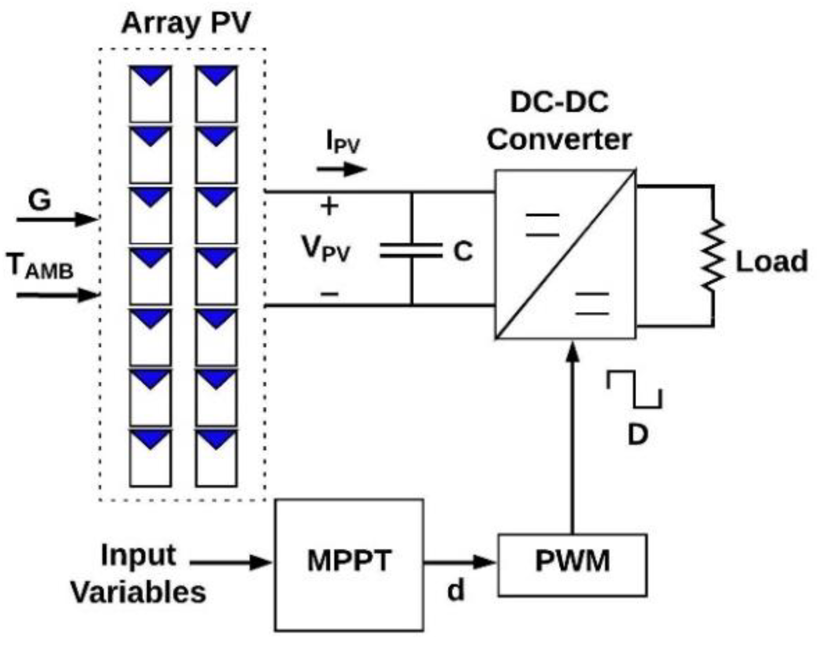
2. Photovoltaic System

The block diagram of the photovoltaic system adopted for this research is shown in Figure 1. It comprises 14 series-connected PV modules, a buck–boost DC–DC converter, an MPPT algorithm, and a load. A capacitor between the PV array and DC–DC converter reduces noises [28].

Figure 2 shows the installation of the PV array used in this research. The PV system is installed at the Federal Rural University of the Semi-Arid (UFERSA), located in the city of Mossoró (5°11′17″ S, 37°20′39″ W). Mossoró belongs to the Fortaleza time zone (Greenwich Mean Time (GMT)—3 h). The system is a 3 kWp PV plant.

The PV module modeling and buck–boost converter components are discussed in Section 2.1 and Section 2.2, respectively. The MPPT algorithm developed will be explained in a separate section.

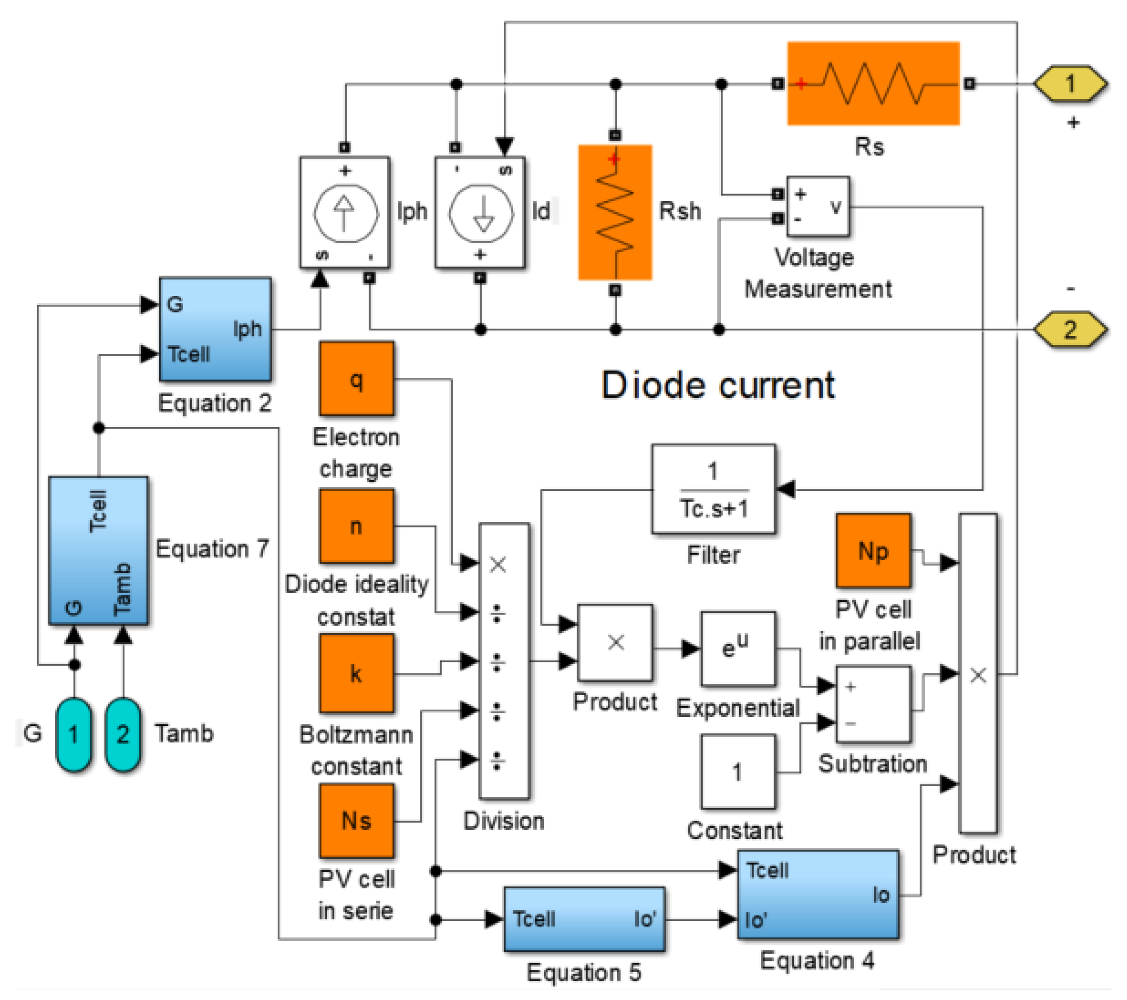
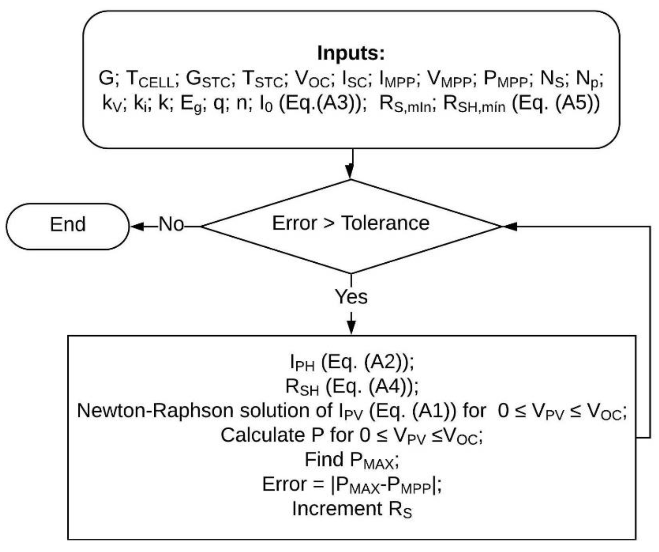
2.1. PV Module Modeling

The current extracted from each PV module is based on the single-diode model. The model was exhaustively discussed in [29]. The diode ideality constant (n) used in the model was empirically chosen as 1 to improve the model fit.

Some authors have investigated how to estimate the ideality factor n [30,31]. In the context of this work, this constant was considered as 1 ≤ n ≤ 1.5 [29]. Villalva, Gazoli, and Ruppert Filho [29] clarified that designers should choose n to improve the model fit so that it is close to the data provided by the manufacturer.

Another essential variable of PV module modeling is defining the PV cell temperature because the diode reverse saturation current (I_o) of the single-diode model depends on the cell temperature (T_CELL). There is no temperature sensor at the PV cell p–n junction, and placing this sensor is complex. The PV cell temperature varies with the ambient temperature and irradiance [32]. Thus, as a solution, it is possible to employ Equation (1) to find the PV cell temperature.

$$T_{CELL}=T_{AMB}+\frac{G}{800}\left(NOCT-20\right)+273,$$

(1)

where T_AMB is the ambient temperature in (°C), and NOCT is the nominal operating cell temperature (°C).

The nominal operating cell temperature (NOCT) is a parameter offered by the manufacture and represents the PV cell temperature measured when T_AMB is 20 °C, G is 800 W/m², and the wind speed is 1 m/s [32]. This parameter links the PV cell temperature and weather conditions (T_AMB and G).

The studied PV system operates with the YL245P-29b PV module model.

Table 1. Parameters of the PV module.

Parameter	Value	Parameter	Value	Parameter	Value	Parameter	Value
VOC	37.5 V	kV	−0.1248 V/K	NP	1	VMPP	29.6 V
ISC	8.83 A	NOCT	46 °C	PMPP	245 W	RSH	404.1 Ω
ki	0.004415 A/K	NS	60	IMPP	8.26 A	RS	0.411 Ω

describes the parameters extracted from the manufacture’s datasheet [33].

The manufacture’s datasheet does not provide the R_SH and R_S values. Therefore, the R_SH and R_S model parameters were calculated (see Table 1 and Appendix A).

The methods to extract the model parameters have been extensively explored in the literature [34,35,36]. Nevertheless, most of them demand sensing and equipment, or even data that are not always available. Therefore, the method chosen was developed by Villalva, Gazoli, and Ruppert Filho [29]. It is an efficient and consolidated method and requires just the data available on the manufacturer’s datasheet. The method is explained in Appendix A.

Figure 3 shows the developed model using MATLAB/Simulink^® software. The green blocks are input variables, the yellow blocks are output variables, the orange blocks are PV module parameters, and the blue blocks are masks containing equations developed and discussed previously. Furthermore, a first-order filter was employed as a feedback transfer function to avoid a loop error [37]. T_C is the filter time constant, and the T_C value is equal to the sample time.

After defining the PV module modeling, fourteen PV modules were series connected using MATLAB/Simulink^® to form the 3 kWp PV array, similar to the real PV system. Section 2.2 describes the components of the buck–boost DC–DC converter.

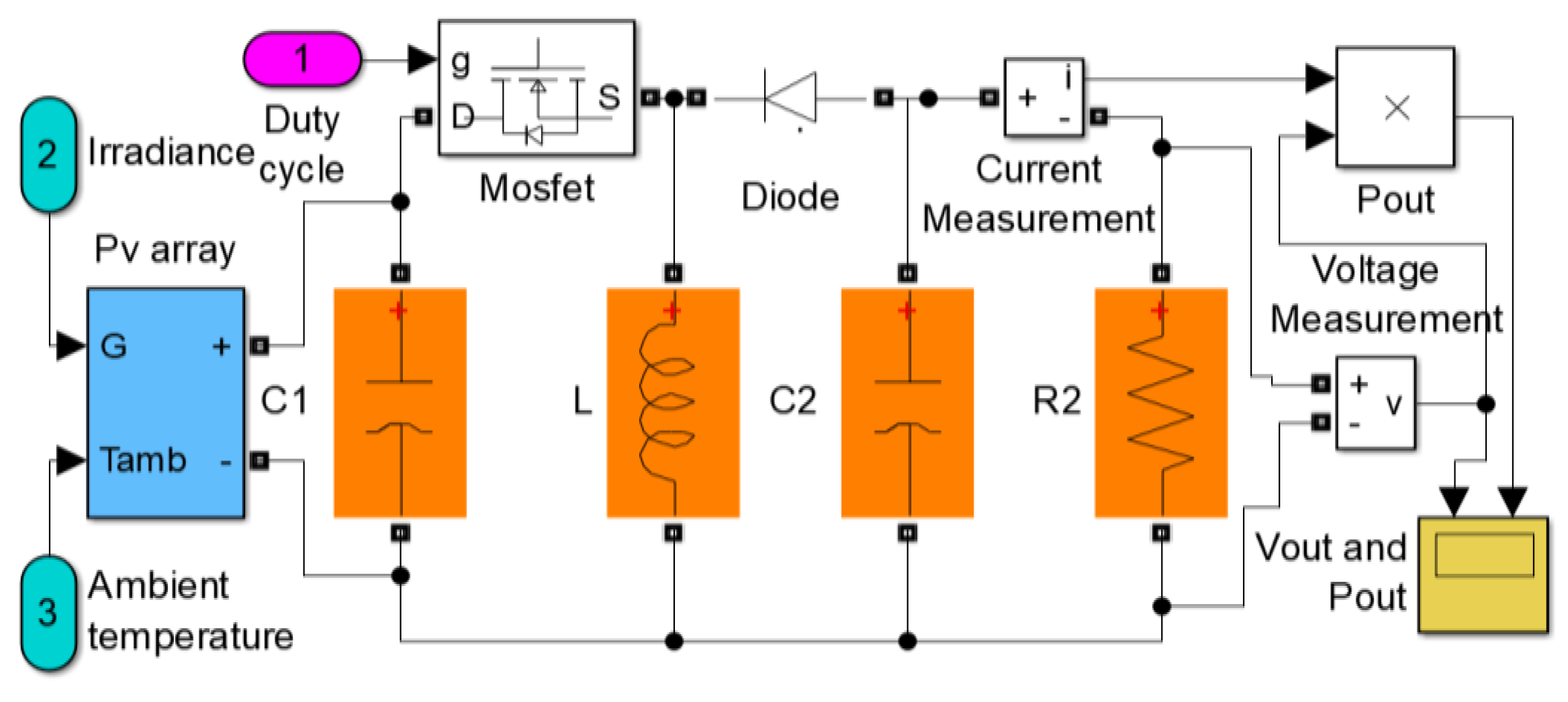
2.2. Buck–Boost Converter

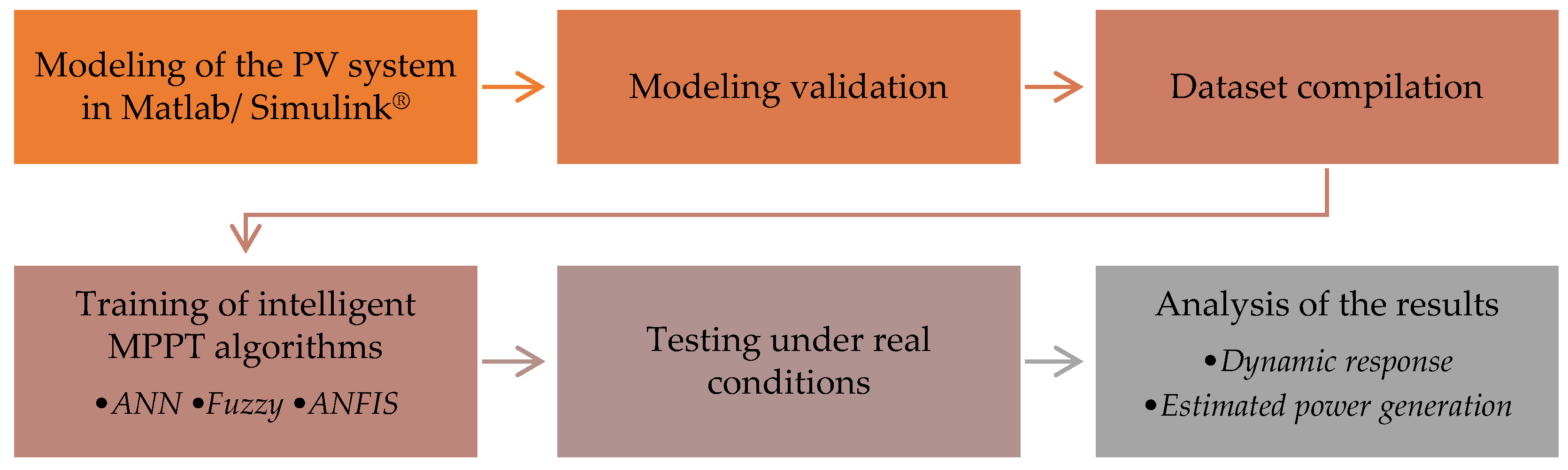
A buck–boost converter is essentially composed of a switching device, a capacitor (C), and an inductor (L) [18]. The MOSFET (metal–oxide–semiconductor field-effect transistor) was chosen as a switching device since it operates at a high frequency, avoiding audible noise. Additionally, a PWM (pulse width modulation) signal is responsible for turning these switches on and off. Therefore, the MPPT algorithm is responsible for controlling the PWM duty cycle (D).

Figure 4 shows the scheme of the buck–boost converter modeled in MATLAB/Simulink^®. The buck–boost converter and the mask representing the PV array (in blue) are connected. Moreover, an input capacitor (C₁) is inserted to reduce oscillations.

The components (in orange) have a recommended minimum value obtained by calculation.

Table 2. Parameters of the buck–boost converter by scenario.

Parameter	Value	Parameter	Value	Parameter	Value
PV module	14	VOUT = VR	480 V	C1 = C2	$20\mathsf{\mu }\mathrm{F}$
PMPP	3430 W	R	67.15 Ω	f	50 kHz
VIN = VMPP	414.4 V	L	5.6 mH	∆IMAX = ∆VMAX (Ripple)	10%

shows the final values chosen. Furthermore, the output variable of the PV system is in yellow, and the PWM duty cycle is in pink.

After modeling the buck–boost converter and defining the load, Section 3 discusses the MPPT algorithms developed and used to control the converter.

3. Methodology

To develop the proposed research, it was necessary to divide the work into six stages. Figure 5 illustrates the methodological structure of the study.

The modeling of the PV system in Matlab/Simulink^® under ambient conditions is shown in Section 2. Therefore, to validate this modeling, the output power was compared in the real PV system with the P_MPP of the modeling in MATLAB/Simulink^® software. The systems with different MPPT techniques were submitted to the same ambient conditions. Afterwards, the simulation dataset was expanded to conduct the third step of the methodology (Figure 5).

The G parameter varies between 100 and 1100 W/m², with a step of 100 W/m². Likewise, the T_AMB parameter considers temperature values between 15 and 45 °C, with an increment of 5 °C. In contrast, the D parameter was calculated.

For each G and T_AMB value, P_MPP was extracted. Therefore, knowing the fixed load value, the maximum power point voltage (V_MPP) was calculated using Equation (2). V_MPP is the output voltage of the PV system.

$$V_{MPP}=\sqrt{R.P_{MPP}}$$

(2)

where R is the load in (Ω) (Table 2), V_MPP is the maximum power point voltage in (V), and P_MPP is the maximum power point power in (W).

After, the duty cycle (D) was calculated for each pair of ambient conditions G and T_AMB using Equation (3).

$$D=\frac{\left|V_{OUT}\right|}{V_{IN}+\left|V_{OUT}\right|},$$

(3)

where V_OUT is V_MPP or the buck–boost output voltage in (V), and V_IN is the buck–boost input voltage in (V). V_IN was extracted from the MATLAB/Simulink^® simulation.

With 77 combinations of G and T_AMB, 77 duty cycle values were obtained. D ranged from 0.2582 to 0.6193. Therefore, the dataset of this paper is a compilation of parameters G, T_AMB, and D. At the end of the compilation, a dataset with 77 samples was obtained to train AI techniques used as an MPPT algorithm in this research.

The fourth step is the modeling and training of the MPPT algorithms. Artificial intelligence techniques are used as MPPT algorithms since they can deal with the nonlinearity, complexity, and uncertainties of these systems, often through robust and low-cost solutions [2]. In this study, the ANN, fuzzy logic, and ANFIS MPPT algorithms were used in the PV system (Figure 1).

The MPPT algorithm models use the G and T_AMB as input variables. The output variable is the duty cycle D. Figure 6 illustrates the scheme developed in MATLAB/Simulink^® for all proposed MPPT algorithms in this study.

Empirically, the switching frequency chosen for the PWM generator (Figure 6) was 50 kHz. The sampling time rate had its value established as the inverse frequency, i.e., 20 μs. The “Unit Delay” blocks (Figure 6) represent the signal discretization.

Finally, it is necessary to train the intelligent algorithms using a dataset with 77 samples. The training of the ANN, FL, and ANFIS algorithms is described in Section 3.1, Section 3.2, and Section 3.3, respectively.

3.1. MPPT Algorithms Based on ANN

Artificial neural networks (ANNs) are computational models inspired by the human brain. They are composed of a set of processing units known as artificial neurons. The synaptic weight vectors interconnect these artificial neurons [38].

In MPPT applications, the most common ANN used is the multilayer perceptron with a feed-forward architecture, usually with three layers: an input layer, a hidden layer, and an output layer. Moreover, the performance function of the network is the mean square error (MSE) [38].

The ANN was trained using the MATLAB/Simulink^® software. All considered scenarios used 70% of the data points for training, 15% of the data points for validation, and 15% of the data points for testing.

Table 3. Main parameters of the ANN.

Parameter	Data	Parameter	Data
Network type	Multilayer Perceptron	Number of neurons	(5,1)
Training algorithm	Levenberg–Marquardt	Activation function	(tansigmoid, pureline)
Inputs	[G TAMB]	Number of samples in dataset	77
Outputs	[D]	Epochs	9
Number of layers	2	MSE	$2.4677\times {10}^{-8}$
R2	1

shows some parameters used for training the ANN.

3.2. MPPT Algorithms Based on Fuzzy Logic

The most critical aspect of fuzzy logic (FL) is converting inaccurate and qualitative information into numerical values. When applied to PV systems as an MPPT control algorithm, FL stands out for not needing an accurate mathematical model and dealing with the nonlinearity of the PV system [39].

The MPPT training based on FL used 11 triangular membership functions (MFs) for the G input variable, 7 triangular MFs for the T_AMB input variable, and 5 triangular MFs for the D output variable.

After establishing the MFs, IF/THEN statements were used to define the FL system rules.

Table 4. Rule base matrix of a fuzzy controller.

	Input 2	15 [15 15 20]	20 [15 20 25]	25 [20 25 30]	30 [25 30 35]	35 [30 35 40]	40 [35 40 45]	45 [40 45 45]
Input 1
100 [100 100 200]		LO	LO	LO	LO	LO	LO	LO
200 [100 200 300]		LO	ML	ML	ML	ML	ML	ML
300 [200 300 400]		ML	ML	ML	ML	M	M	M
400 [300 400 500]		M	M	M	M	M	M	M
500 [400 500 600]		M	M	M	M	MH	MH	MH
600 [500 600 700]		MH	MH	MH	MH	MH	MH	MH
700 [600 700 800]		MH	MH	MH	MH	MH	MH	MH
800 [700 800 900]		MH	MH	MH	H	H	H	H
900 [800 900 1000]		H	H	H	H	H	H	H
1000 [900 1000 1100]		H	H	H	H	H	H	H
110 [1000 1100 1100]		H	H	H	H	H	H	H

shows the input MF settings and the fuzzy rules applied.

Overall, the Mamdani fuzzy controller employed 77 fuzzy rules.

Table 5. Parameters of the fuzzy controller with the input variables G and T_AMB.

Parameter	Data	Parameter	Data	Parameter	Data
Type	Mamdani	Number of rules	77	Output range	[0.2582 0.6193] LO = [0.2583 0.3 0.34] ML = [0.331 0.3897 0.41] M = [0.4028 0.44 0.475] MH = [0.47 0.5085 0.547] H = [0.54 0.58 0.6195]
Inputs	[G TAMB]	Type of input MF	trimf
Output	[D]	Type of output MF	trimf
Number of input MFs	[11 7]	Input range 1	[100 1100]
Number of output MFs	5	Input range 2	[15 45]

summarizes the main characteristics that set up the modeled fuzzy controller.

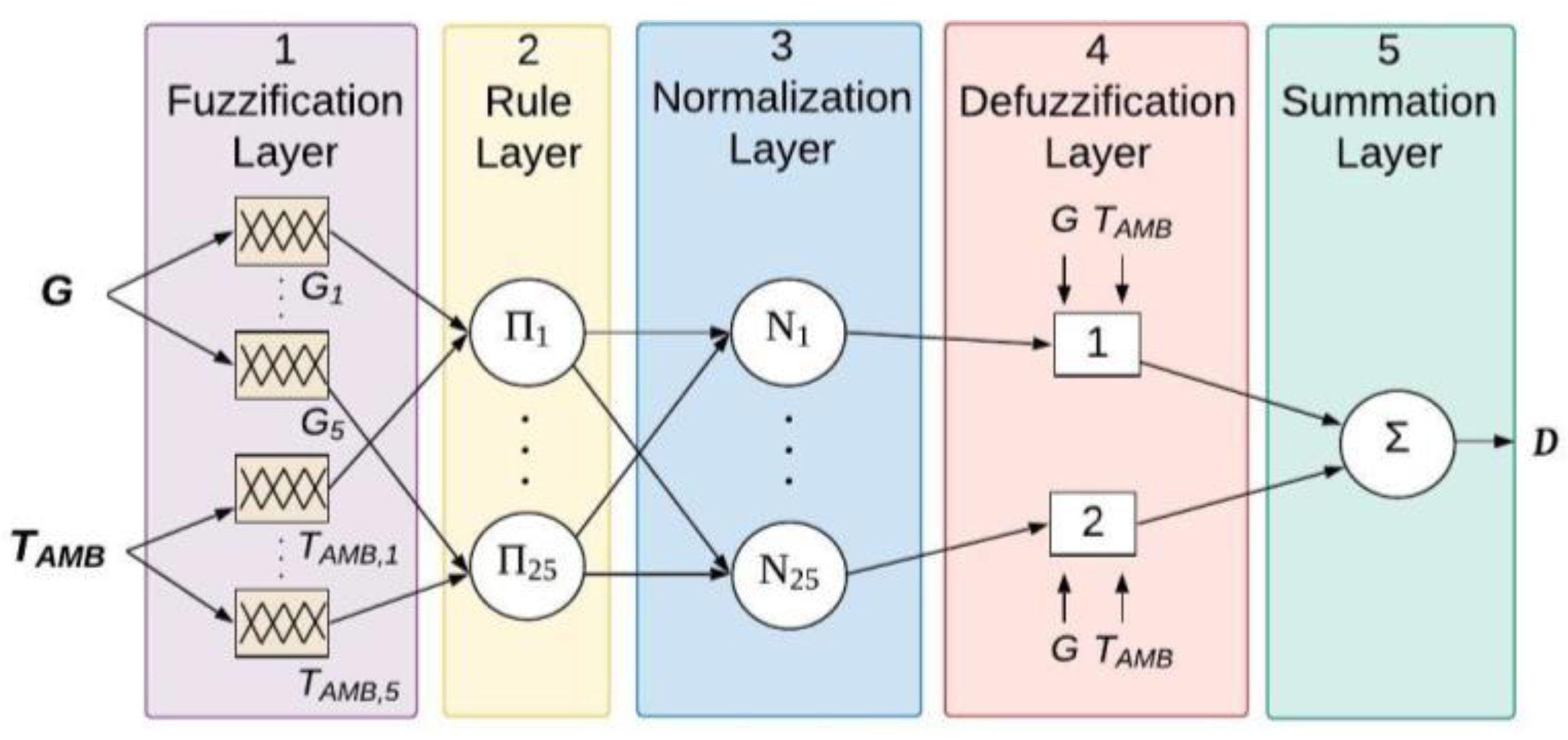
3.3. MPPT Algorithms Based on ANFIS

Adaptive neuro-fuzzy inference systems (ANFISs) are hybrid intelligence techniques that combine ANN and FL techniques. In an ANFIS, a particular ANN architecture incorporates a fuzzy inference system (FIS). Therefore, the fuzzy controller receives a learning algorithm [40].

However, when comparing it to other conventional MPPT techniques, ANFIS as an MPPT control algorithm applied to PV systems is still recent. Thus, this study modeled the ANFIS MPPT using the MATLAB/Simulink^® software.

The ANFIS was trained using all 77 samples of the dataset. In the ANFIS architecture, each input has 5 triangular MFs, totaling 25 fuzzy rules. The output is a constant MF. Figure 7 illustrates the architecture scheme.

Finally,

Table 6. The main parameters of the ANFIS algorithm with the G and T_AMB input variables.

Parameters	Data	Parameters	Data
Type	Sugeno	Type of output MF	constant
Inputs	[G TAMB]	Input range 1	[100 1100]
Output	[D]	Input range 2	[15 45]
Number of input MFs	[5 5]	Output range	[0.2582 0.6193]
Number of output MFs	25	Training	hybrid
Number of rules	25	Iterations	3
Type of input MF	trimf

briefly presents the main parameters of the ANFIS technique used as an MPPT control algorithm for the PV system.

After modeling the MPPT algorithms, the PV systems were simulated considering different ambient conditions. Section 4 describes the ambient conditions used in the simulation, and it discusses the testing results.

4. Results and Discussion

Firstly, the PV system modeling is validated in Section 4.1. Then, ambient conditions are defined empirically (Section 4.2) to later analyze the dynamic response of the output power of the systems in Section 4.3 and Section 4.4. Finally, the power generated by each PV system is calculated in Section 4.5, and a critical analysis is carried out.

4.1. Validation of the Modeled PV System

Primarily, the simulation results were compared with the values measured experimentally to validate the PV system modeling of Section 2. In this analysis, six real and random ambient conditions were chosen. The comparison was between the model simulation and the real PV system P_MPP output powers.

Table 7. Output power in the real PV system and the MPP of the modeled PV system.

Conditions	Ambient Conditions		Real System	Simulated System
	G (W/m2)	TAMB (°C)	Pmeasured (W)	PMPP,simulation (W)	e%
1	294	23.86	919.25	935.2	1.73
2	303	31.74	906.83	893.9	1.43
3	548	24.65	1664.60	1629.0	2.14
4	868	31.46	2099.38	2105.0	0.27
5	957	31.41	2198.76	2223.0	1.10
6	1134	30.17	2397.52	2438.0	1.69

shows the comparative results.

Observing Table 7, the modeled PV system presented results close to the values measured experimentally for all ambient conditions. Furthermore, the relative errors of the powers were between 0.27% and 2.14%. Therefore, the modeling developed in Section 2 estimated correct parameters because the simulation returned results consistent with reality. Thus, it was appropriate to use the model for the elaboration of the dataset and subsequent simulation.

For the simulations, the ambient conditions needed to be defined, as shown in Section 4.2.

4.2. Definition of Ambient Conditions

The control algorithms from the PV system were connected separately considering the same ambient conditions to analyze the dynamic response of the output power.

Table 8. Ambient conditions and respective expected P_MPP.

Condition	G (W/m2)	TAMB (°C)	PMPP (W)
Condition 1	303	24	961.5
Condition 2	631	32	1684.0
Condition 3	957	32	2205.0
Condition 4	548	24	1640.0

details the randomly chosen ambient conditions.

Table 8 also shows the expected P_MPP in the output of the PV system. It is worth highlighting that the change in ambient conditions considers the cloud edge effect.

After estimating the expected power, the convergence speed, tracking accuracy, and oscillation around the MPP parameters were verified and are discussed in Section 4.3 and Section 4.4. These parameters make up the dynamic response of the output signal. A comparison between the intelligent and classic P&O algorithms was also performed.

Afterwards, the PV systems were subjected to three ambient conditions of the city used in this paper. The city is located near the Equator (5°11′17″ S, 37°20′39″ W), GMT-3. This city has a dry and sunny tropical climate. The extracted conditions were irradiance and ambient temperature, and the ambient conditions are explained in Section 4.2.1, Section 4.2.2, Section 4.2.3.

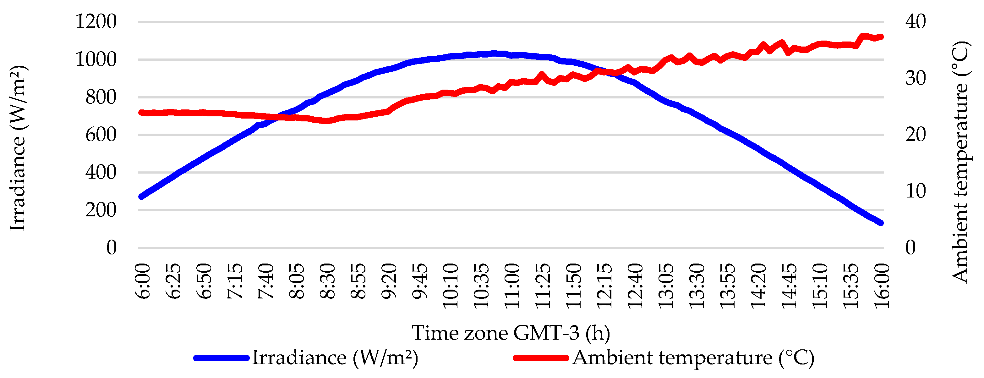
4.2.1. Normal Condition

A day in normal conditions has a full sun and a clear sky. Therefore, the irradiance increases until close to 12:00 h (GTM-3) and exceeds 1000 W/m² in the region of this research. After midday, the irradiance declines until sunset. Conversely, the ambient temperature only increases on this type of sunny day. Figure 8 illustrates the ambient condition of the normal condition scenario.

4.2.2. Shading Condition

In the shading condition, it is possible to observe a behavior of the ambient temperature similar to that of the normal condition (Section 4.2.1). However, the irradiance has an actual and rapid drop near 11:00 h (GTM-3), as shown in Figure 9. This sudden change in irradiance levels is a consequence of passing clouds.

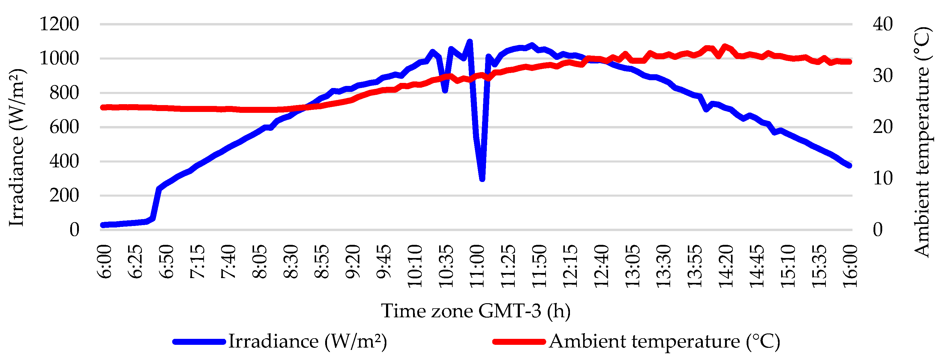
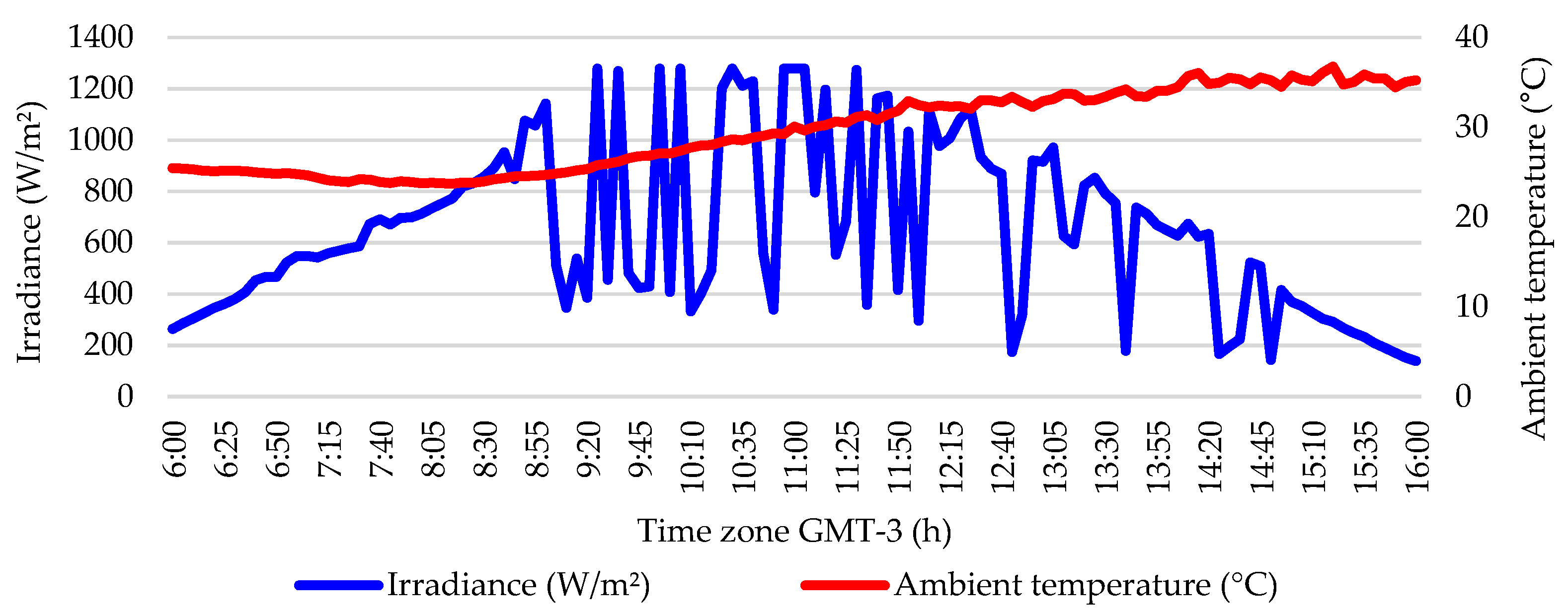
4.2.3. Forecasting Condition

The forecasting condition is defined as the situation in which solar irradiance changes over time. The ambient temperature maintains the performance of only increasing throughout the day. Figure 10 shows the G and T_AMB conditions.

In Section 4.5, the power generated by each PV system is calculated and, finally, compared with a PV system with MPPT based on P&O.

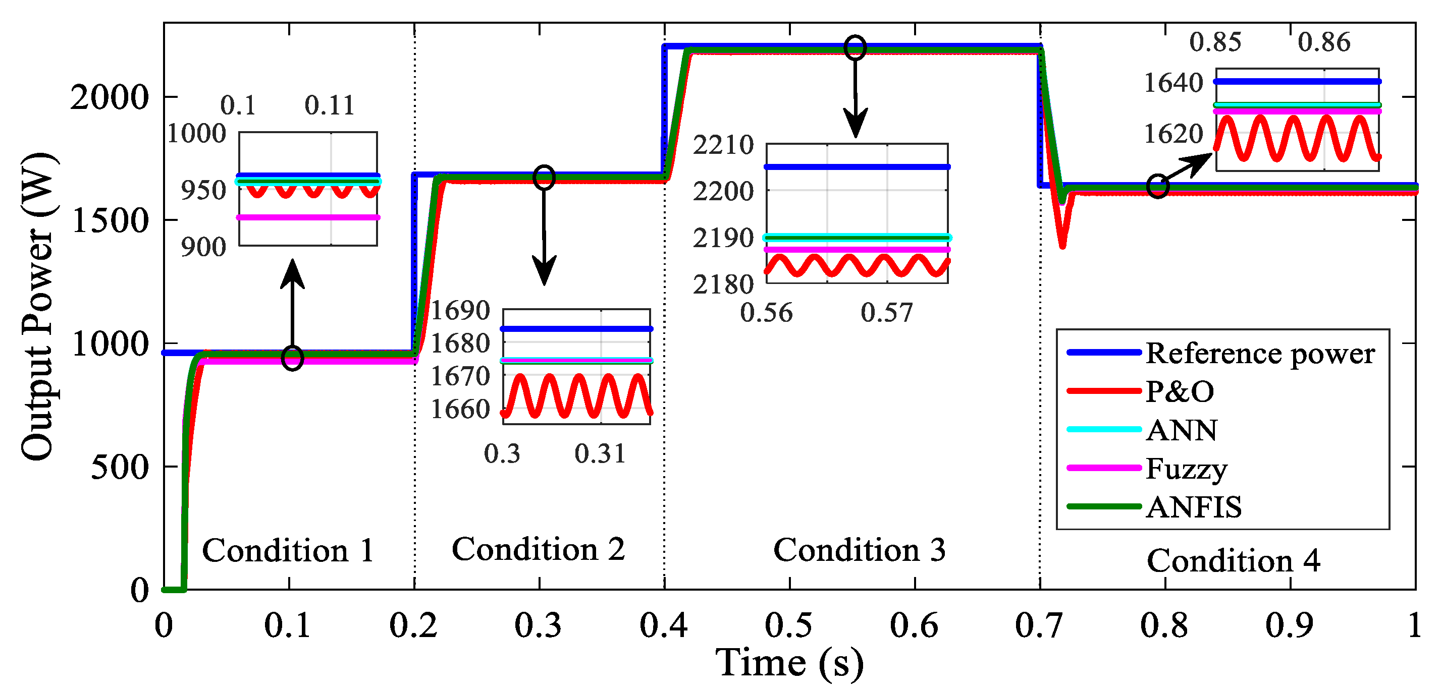
4.3. Dynamic Response Analysis

Each intelligent MPPT technique modeled and connected to the PV was submitted to the ambient conditions of Table 8. Therefore, the dynamic response of the output power was analyzed. In Figure 11, the blue curve is the expected P_MPP value for each ambient condition.

Analyzing Figure 11, the ANFIS and ANN algorithms were faster in achieving the steady state. On the other hand, the P&O algorithm was the slowest technique. Additionally, the P&O algorithm presented more significant oscillations around the MPP in the steady state when compared to the intelligent algorithm used as an MPPT control technique.

The convergence speed is the time that the PV system takes to achieve the steady state. Therefore, the settling time (ts) was the chosen parameter. The oscillation around the MPP (∆P) is the peak-to-peak value of the signal in the steady state. Finally, ∆P is the ratio between the peak value and the average value of the output power measured in the steady state.

Table 9. The settling time and the oscillation around the MPP parameters.

Condition	ts (ms)				∆P (%)
	P&O	ANN	FUZZY	ANFIS	P&O	ANN	FUZZY	ANFIS
1	29.16	23.44	22.24	23.54	0.57325	0.00020	0.00012	0.00016
2	19.90	15.60	15.70	15.8	0.33984	0.00031	0.00012	0.00028
3	15.70	14.10	14.10	14.3	0.00872	0.00023	0.00012	0.00026
4	22.50	13.40	13.20	13.0	0.22308	0.00011	0.00013	0.00013

describes the settling time (ts) and the oscillation around the MPP (∆P) parameters.

The settling time of the P&O algorithm (Table 9) was longer than that of all simulated intelligent techniques, as observed in Figure 11. Overall, the ANFIS, ANN, and fuzzy algorithms showed similar settling times. Intelligent algorithms were at least 1 ms faster than the classic P&O algorithm. The lowest difference among settling times of the algorithms occurred in Condition 3.

The oscillation around the MPP (∆P) of the intelligent techniques (ANN, fuzzy, and ANFIS) is almost undetectable because they correspond to a variation of less than 0.001%. In contrast, the P&O shows oscillations around the MPP between 0.008% and 0.57%. Therefore, expanding on the graph of Figure 11, fluctuations of the P&O algorithm are observed, while the intelligent algorithms’ signals do not seem to exhibit oscillation in the steady state.

Moreover, the parameter used to verify the tracking accuracy is the relative percentage error. This error compares the average power value of the PV system in the steady state with the expected P_MPP established in Table 8.

Table 10. The average power of the PV system in the steady state, and the respective relative percentage error.

Condition	PMPP (W)	P&O		ANN		FUZZY		ANFIS
		PP&O (W)	e%	PANN (W)	e%	PFUZZY (W)	e%	PANFIS (W)	e%
1	961.5	951.6	1.03	956.5	0.52	924.9	3.81	956.6	0.51
2	1684.0	1664.0	1.19	1674.0	0.59	1674.0	0.59	1674.0	0.59
3	2205.0	2184.0	0.95	2190.0	0.68	2187.0	0.82	2190.0	0.68
4	1640.0	1618.0	1.34	1631.0	0.55	1628.0	0.73	1631.0	0.55

and Figure 12 show the results obtained with MPPT based on each AI technique. The results were also compared to the classic P&O technique.

Table 10 and Figure 12 show that MPPT based on intelligent algorithms showed a better tracking accuracy than that with the classic P&O algorithm. Furthermore, the ANFIS and ANN algorithms showed better precision or a reduced relative percentage error.

Additionally, under low irradiance (Condition 1—Figure 12a), the relative percentage error of the FL algorithm (3.81%) was higher than that of the P&O algorithm (1.03%). Therefore, the FL algorithm needs a fine adjustment and, consequently, more knowledge of the expert operators.

This research observed that the ANN and ANFIS algorithms perform better than the P&O and FL algorithms when the dynamic response is analyzed. Additionally, it was observed that the ANN and ANFIS algorithms did not need to carry out several tests to find the optimal structure during the training phase.

In contrast, while MATLAB/Simulink^® software defines the ANFIS MFs, the expert operator must establish the fuzzy MFs. Therefore, reducing the number and changing the type of ANFIS MFs was faster and easier than those for the fuzzy MFs. Consequently, the ANFIS algorithm needs less computational effort to control the MPPT of the PV system.

Analyzing the simplicity of implementation, the ANN and fuzzy algorithms have a medium complexity. On the other hand, the ANFIS algorithm has a high complexity and requires features such as high-performance controllers. Therefore, while the ANFIS and ANN algorithms have a similar dynamic response, the ANN algorithm is better as it is more robust.

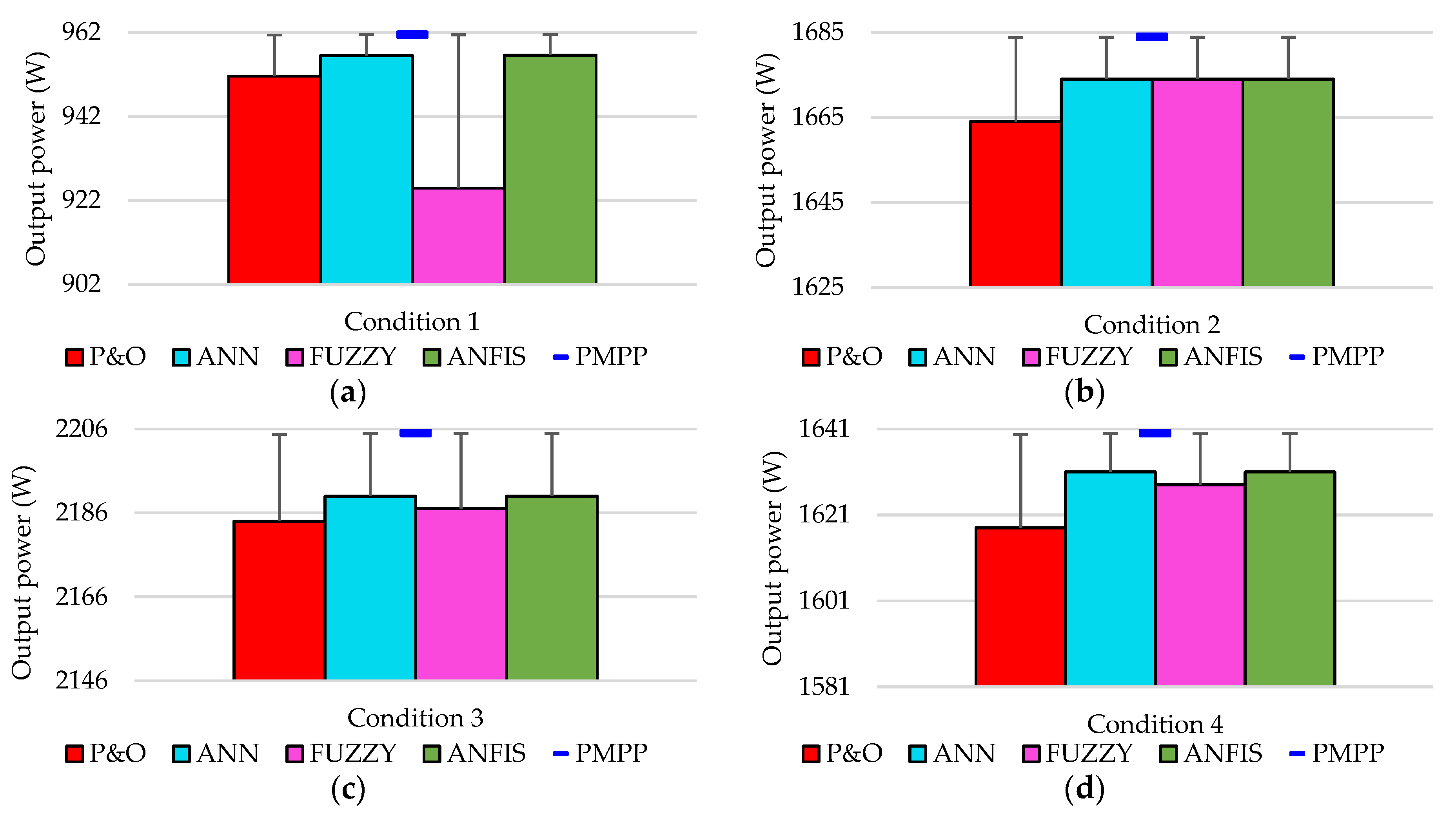
4.4. Comparative Study

Few studies using buck–boost as an MPPT converter were found in the literature. Anyway,

Table 11. Comparison with other published studies.

Reference	Algorithm	Settling Time (ms)	Accuracy (%)	Experimentally Tested	Dataset
Proposed research	ANN	13.40–23.44	99.32–99.48	No	77
	Fuzzy	13.20–22.24	96.19–99.41
	ANFIS	13.00–23.54	99.32–99.49
Aldobhani and John [7,8]	ANFIS	-	98–99	No	39
Panda, Pathak, and Srivastava [10]	Fuzzy	12.20	-	No	-
Arora and Gaur [16]	ANN	125.00	99.83	No	300,001
	ANFIS	105.00	100
Martin and Vazquez [17]	Fuzzy	-	98.2	Yes	-
	ANFIS	-	98.2
Belhachat and Larbes [18]	ANFIS	-	99.92	No	-
Andrew-Cotter, Uddin, and Amin [26]	ANFIS	-	97	No	-

evaluates and performs a reasonable comparison of the proposed research results with previously published studies.

Table 11 describes the type of algorithm, the settling time, and the method’s accuracy. All missing data in papers are hyphenated in Table 11.

Among the research that used buck–boost as an MPPT converter, only two works measured the settling time. The Panda, Pathak, and Srivastava [10] study achieved a settling time close to the method proposed in the present paper. The time value is even shorter due to the smaller variations in the ambient conditions that the Panda, Pathak, and Srivastava [10] PV system was subjected to.

In contrast, the settling time of the Arora and Gaur [16] system was considerably longer than that of the proposed research. The difference can be explained because the Arora and Gaur [16] system had been connected to the grid and subjected to a slow, graded range of changing solar irradiation levels.

With respect to the accuracy, the results show that the intelligent algorithms have the best accuracy in following the MPP of the PV module compared to the P&O algorithm. As discussed in Section 1 and Section 3, this result was expected because AI techniques work better with nonlinear systems than classic techniques [3,4].

In the proposed fuzzy research, the lowest accuracy was detected among intelligent algorithms. This means the MFs and fuzzy rules directed to low irradiances need to be adjusted.

The results also show that the performance of the MPPT algorithm depends more on the quality than the quantity of the training data [41]. Specifically, assessing the Arora and Gaur [16] results, they calculated the accuracy based on the maximum power output of the PV module. The other papers of Table 11 were evaluated based on the MPP of the P–V characteristic curve.

The present paper proposes evaluating the replacement of the classic P&O algorithm with an intelligent algorithm. Therefore, after analyzing the dynamic response advantages of intelligent algorithms, it is known that the dynamic response influences the generated PV system power. Therefore, estimating the power generation of the PV system is as crucial as analyzing the dynamic response.

In the literature, no research was found that performed a comparative analysis of the generated power. Thus, Section 4.5 evaluates the power generation of the PV system with intelligent and classic MPPT techniques.

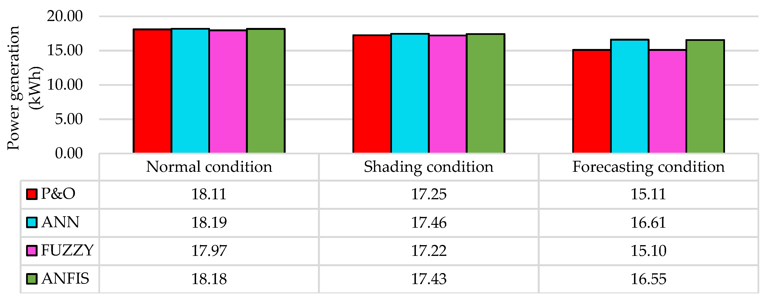
4.5. Estimated Power Generation

The estimated power generation used three ambient conditions for the PV system, called the normal condition (Figure 8), shading condition (Figure 9), and forecasting condition (Figure 10). In addition, ten hours of full sun on both days, i.e., from 6:00 a.m. to 4:00 p.m., was considered. Figure 13 shows the result of estimating the power generation of the PV system considering the different control algorithms.

The power generation of the PV system with the P&O algorithm (Figure 13) was considered as the reference of the energy produced, i.e., it corresponds to 100% of the power generation in the experimental PV system. Therefore, replacing the P&O algorithm with the ANN algorithm allows recovery of 0.46% of the power generation in the normal condition. If replaced by the ANFIS algorithm, the energy recovery is 0.40%. However, if the control algorithm of MPPT is fuzzy, there is an energy loss of 0.75%.

In the shading condition, there is a rapidly changing irradiance near noon. Consequently, the good dynamic response of the intelligent algorithm helps to improve the recovery of the power generated.

Observing Figure 13, the exchange of the P&O algorithm for the ANN algorithm recovers the power generated by the PV system. To be precise, the power generation of the PV system with ANN is 1.21% greater than with P&O. The energy recovery is 1.02% when the P&O algorithm is replaced with the ANFIS algorithm.

Otherwise, when the P&O algorithm is substituted for the fuzzy algorithm, there is a loss of power generation by 0.19%. In other words, the PV system with MPPT based on FL generated less power than that based on P&O. Specifically, the fall in the power generation was from 17.25 to 17.22 kWh. A similar performance of the fuzzy algorithm was observed in the forecasting condition. MPPT based on FL showed a reduction from 15.11 to 15.10 kWh, i.e., it fell 0.04%.

Additionally, in the forecasting condition, the power generation recovery was more expressive. When the P&O algorithm was changed for the ANN algorithm, the performance was better because the power generation increased from 15.11 to 16.61 kWh, i.e., 9.9%.

The ANFIS algorithm’s performance was as good as the ANN algorithm’s performance. The power generation rose 9.53%, which means that the power generation grew from 15.11 (with P&O) to 16.55 kWh.

Thus, these analyses allow concluding that intelligent MPPT techniques could track the MPP with an excellent dynamic response. Furthermore, the PV system with MPPT based on the ANN algorithm was remarkably useful in tracking the maximum power point in the PV system. MPPT based on ANN can recover lost energy generated with MPPT based on P&O.

Finally, Section 5 discusses the overall conclusion of this research.

5. Conclusions

Using buck–boost converters as an MPPT component of PV systems is uncommon, but they are important for regions with a dry and sunny tropical climate. In this research, intelligent algorithms were applied to control MPPT, and ambient conditions (G and T_AMB) were considered as input variables. No similar discussion in the scientific literature has been found.

The simulations demonstrated the potential effectiveness of the PV system with MPPT based on intelligent techniques, and the following conclusions can be drawn:

• The proposed ANN and ANFIS MPPT techniques are considered an improvement of the classic P&O technique. If considering large-scale PV plants, they cause a subsequent increase in power generation.
• For all considered environmental conditions, the PV system with MPPT based on intelligent techniques achieved values close to the expected P_MPP. Therefore, these techniques were able to track the MPP with great accuracy.
• A high tracking speed was also observed because the intelligent algorithm localized the true P_MPP quickly in every irradiance change.
• Intelligent techniques showed negligible oscillations around the average power value in the steady state, when compared to the classic P&O technique. The amplitude of the oscillation is reflected in the system stability.
• The fuzzy intelligent technique showed less satisfactory results than the ANN and ANFIS techniques. However, more knowledge of the expert operators and a fine adjustment in the fuzzy controller parameters can improve the output power of the PV system with MPPT based on FL.
• Submitting the modeled PV system to ambient conditions of regions close to the Equator line, a more significant power generation was observed when using the ANN and ANFIS intelligent algorithms in the MPPT of the PV system. The power recovery was between 0.40% and 9.9%.
• The power recovery of the PV system with MPPT based on the ANN or ANFIS algorithm exceeded 1% when the ambient condition had a rapidly falling irradiance near noon in the shading condition. Furthermore, the power recovery achieved 9.9% in the forecasting condition (when the solar irradiance changes over time). The better dynamic response of these intelligent algorithms than that of the fuzzy and P&O algorithms justifies this recovery of power generation.
• Among the intelligent techniques simulated in the present paper, the ANN and ANFIS algorithms had a similar response. However, the ANN technique proposed a higher power generation. Moreover, the ANN algorithm has a less complex implementation, and it is more robust to noise.
• Using environmental parameters G and T_AMB as input variables has the advantage of being able to track the MPP regardless of the geographic location of the PV system. Moreover, the global maximum power point is followed with high reliability. However, its cost of implementation and applicability remain a challenge due to the increased cost of implanting the sensors.

References

1. Hanzaei, S.H.; Gorji, S.A.; Ektesabi, M. A Scheme-Based Review of MPPT Techniques With Respect to Input Variables Including Solar Irradiance and PV Arrays’ Temperature. IEEE Access 2020, 8, 182229–182239. [Google Scholar] [CrossRef]
2. Sumathi, S.; Ashok Kumar, L.; Surekha, P. Solar PV and Wind Energy Conversion Systems; Springer: Cham, Switerland, 2015; ISBN 978-3-319-14940-0. [Google Scholar]
3. Youssef, A.; El-Telbany, M.; Zekry, A. The role of artificial intelligence in photo-voltaic systems design and control: A review. Renew. Sustain. Energy Rev. 2017, 78, 72–79. [Google Scholar] [CrossRef]
4. Vieira, G.; Ugulino de Araújo, F.M.; Dhimish, M.; Guerra, M.I.S. A Comprehensive Review on Bypass Diode Application on Photovoltaic Modules. Energies 2020, 13, 2472. [Google Scholar] [CrossRef]
5. Enrique, J.M.; Durán, E.; Sidrach-de-Cardona, M.; Andújar, J.M. Theoretical assessment of the maximum power point tracking efficiency of photovoltaic facilities with different converter topologies. Sol. Energy 2007, 81, 31–38. [Google Scholar] [CrossRef]
6. Reshma Gopi, R.; Sreejith, S. Converter topologies in photovoltaic applications—A review. Renew. Sustain. Energy Rev. 2018, 94, 1–14. [Google Scholar] [CrossRef]
7. Aldobhani, A.M.S.; John, R. Maximum Power Point tracking under Different Environment Conditions for Solar Photovoltaic Panels Using ANFIS Model. J. Sci. Technol. 2007, 12, 31–47. [Google Scholar]
8. Aldobhani, A.M.S.; John, R. Maximum Power Point Tracking of PV System Using ANFIS Prediction and Fuzzy Logic Tracking. Lect. Notes Eng. Comput. Sci. 2008, 2169, 1359–1366. [Google Scholar]
9. Otieno, C.A.; Nyakoe, G.N.; Wekesa, C.W. A neural fuzzy based maximum power point tracker for a photovoltaic system. In Proceedings of the IEEE AFRICON Conference, Nairobi, Kenya, 23–25 September 2009; IEEE: Nairobi, Kenya, 2009; pp. 1–6. [Google Scholar]
10. Panda, A.; Pathak, M.K.; Srivastava, S.P. Fuzzy Intelligent Controller for the Maximum Power Point Tracking of a Photovoltaic Module at Varying Atmospheric Conditions. J. Energy Technol. Policy 2011, 1, 6–9. [Google Scholar]
11. Nabipour, M.; Razaz, M.; Seifossadat, S.G.; Mortazavi, S.S. A new MPPT scheme based on a novel fuzzy approach. Renew. Sustain. Energy Rev. 2017, 74, 1147–1169. [Google Scholar] [CrossRef]
12. Ahmed, J.; Salam, Z. A soft computing MPPT for PV system based on Cuckoo Search algorithm. In Proceedings of the 4th International Conference on Power Engineering, Energy and Electrical Drives, Istanbul, Turkey, 13–17 May 2013; pp. 558–562. Available online: https://ieeexplore.ieee.org/document/6635669 (accessed on 5 August 2021). [CrossRef]
13. Bollipo, R.B.; Mikkili, S.; Bonthagorla, P.K. Critical Review on PV MPPT Techniques: Classical, Intelligent and Optimisation. IET Renew. Power Gener. 2020, 14, 1433–1452. [Google Scholar] [CrossRef]
14. Ahmed, J.; Salam, Z. A Maximum Power Point Tracking (MPPT) for PV system using Cuckoo Search with partial shading capability. Appl. Energy 2014, 119, 118–130. [Google Scholar] [CrossRef]
15. Shiau, J.K.; Lee, M.Y.; Wei, Y.C.; Chen, B.C. Circuit Simulation for Solar Power Maximum Power Point Tracking with Different Buck-Boost Converter Topologies. Energies 2014, 7, 5027–5046. [Google Scholar] [CrossRef] [Green Version]
16. Arora, A.; Gaur, P. Comparison of f ANN and ANFIS based MPPT controller for grid connected PV Systems. In Proceedings of the IEEE Indicon 2015, New Delhi, India, 17–20 December 2015; pp. 1–6. [Google Scholar]
17. Martin, A.D.; Vazquez, J.R. MPPT algorithms comparison in PV systems: P&O, PI, neuro-fuzzy and backstepping controls. Proc. IEEE Int. Conf. Ind. Technol. 2015, 2015, 2841–2847. [Google Scholar] [CrossRef]
18. Belhachat, F.; Larbes, C. Global maximum power point tracking based on ANFIS approach for PV array configurations under partial shading conditions. Renew. Sustain. Energy Rev. 2017, 77, 875–889. [Google Scholar] [CrossRef]
19. Karagöz, M.K.; Demİrel, H. A Novel MPPT Method for PV Arrays Based on Modified Bat Algorithm with Partial Shading Capability. Int. J. Comput. Sci. Netw. Secur. 2017, 17, 61–66. [Google Scholar]
20. Belhachat, F.; Larbes, C. A review of global maximum power point tracking techniques of photovoltaic system under partial shading conditions. Renew. Sustain. Energy Rev. 2018, 92, 513–553. [Google Scholar] [CrossRef]
21. Khanam, J.J.; Foo, S.Y. Modeling of a Photovoltaic Array in MATLAB Simulink and Maximum Power Point Tracking Using Neural Network. J. Electr. Electron. Syst. 2018, 7, 1–8. [Google Scholar] [CrossRef]
22. Yap, K.Y.; Sarimuthu, C.R.; Lim, J.M.Y. Artificial Intelligence Based MPPT Techniques for Solar Power System: A review. J. Mod. Power Syst. Clean Energy 2020, 8, 1043–1059. [Google Scholar] [CrossRef]
23. Ahmed, J.; Salam, Z. An Enhanced Adaptive P&O MPPT for Fast and Efficient Tracking Under Varying Environmental Conditions. IEEE Trans. Sustain. Energy 2018, 9, 1487–1496. [Google Scholar] [CrossRef]
24. Ahmad, R.; Murtaza, A.F.; Sher, H.A. Power tracking techniques for efficient operation of photovoltaic array in solar applications—A review. Renew. Sustain. Energy Rev. 2019, 101, 82–102. [Google Scholar] [CrossRef]
25. Kumar, J.; Rathor, B.; Bahrani, P. Fuzzy and P&O MPPT techniques for stabilized the efficiency of solar PV system. In Proceedings of the 2018 International Conference on Computing, Power and Communication Technologies (GUCON), Greater Noida, India, 28–29 September 2018; pp. 259–264. Available online: https://ieeexplore.ieee.org/document/8674909 (accessed on 10 August 2021). [CrossRef]
26. Andrew-Cotter, J.; Uddin, M.N.; Amin, I.K. Particle Swarm Optimization based Adaptive Neuro-Fuzzy Inference System for MPPT Control of a Three-Phase Grid-Connected Photovoltaic System. In Proceedings of the IEEE International Electric Machines & Drives Conference (IEMDC), San Diego, CA, USA, 12–15 May 2019; pp. 2089–2094. [Google Scholar]
27. Rajavel, A.; Rathina Prabha, N. Fuzzy logic controller-based boost and buck-boost converter for maximum power point tracking in solar system. Trans. Inst. Meas. Control 2021, 43, 945–957. [Google Scholar] [CrossRef]
28. Leite, A.C.Q.B.; Salazar, A.O.; Carvalho, J.T. Maximum power point tracker based digital one cycle control applied in PV systems. Renew. Energy Power Qual. J. 2017, 1, 239–244. [Google Scholar] [CrossRef]
29. Villalva, M.G.; Gazoli, J.R.; Filho, E.R. Comprehensive approach to modeling and simulation of photovoltaic arrays. IEEE Trans. Power Electron. 2009, 24, 1198–1208. [Google Scholar] [CrossRef]
30. Bayhan, H.; Bayhan, M. A simple approach to determine the solar cell diode ideality factor under illumination. Sol. Energy 2011, 85, 769–775. [Google Scholar] [CrossRef]
31. Simon, M.; Meyer, E.L. Detection and analysis of hot-spot formation in solar cells. Sol. Energy Mater. Sol. Cells 2010, 94, 106–113. [Google Scholar] [CrossRef]
32. Masters, G.M. Renewable and Efficient Electric Power Systems; Wiley-Interscience, John Wiley & Sons: Hoboken, NJ, USA, 2004; ISBN 3175723993. [Google Scholar]
33. Yingli Solar Datasheet YGE 60 Células Série 2; Yingli Green Energy do Brasil, S.A.: Brazil 2015, 2; Available online: https://www.neosolar.com.br/loja/fileuploader/download/download/?d=0&file=custom%2Fupload%2FFile-1438699024.pdf (accessed on 6 April 2021).
34. Lappalainen, K.; Manganiello, P.; Piliougine, M.; Spagnuolo, G.; Valkealahti, S. Virtual Sensing of Photovoltaic Module Operating Parameters. IEEE J. Photovolt. 2020, 10, 852–862. [Google Scholar] [CrossRef]
35. Spagnuolo, G.; Lappalainen, K.; Valkealaht, S.; Manganiello, P. Photovoltaic Module Parametric Identification. In Proceedings of the 2019 International Conference on Clean Electrical Power (ICCEP), Otranto, Italy, 2–4 July 2019; pp. 302–305. [Google Scholar] [CrossRef] [Green Version]
36. Karatepe, E.; Boztepe, M.; Çolak, M. Development of a suitable model for characterizing photovoltaic arrays with shaded solar cells. Sol. Energy 2007, 81, 977–992. [Google Scholar] [CrossRef]
37. Vieira, R.G.; Dhimish, M.; Ugulino de Araújo, F.M.; Guerra, M.I.S. PV module fault detection using combined artificial neural network and sugeno fuzzy logic. Electronics 2020, 9, 2150. [Google Scholar] [CrossRef]
38. Gupta, A.; Chauhan, Y.K.; Pachauri, R.K. A comparative investigation of maximum power point tracking methods for solar PV system. Sol. Energy 2016, 136, 236–253. [Google Scholar] [CrossRef]
39. Lamamra, K.; Batat, F.; Mokhtari, F. A new technique with improved control quality of nonlinear systems using an optimized fuzzy logic controller. Expert Syst. Appl. 2020, 145, 113148. [Google Scholar] [CrossRef]
40. Meharrar, A.; Tioursi, M.; Hatti, M.; Boudghne Stambouli, A. A variable speed wind generator maximum power tracking based on adaptative neuro-fuzzy inference system. Expert Syst. Appl. 2011, 38, 7659–7664. [Google Scholar] [CrossRef]
41. Kordos, M.; Rusiecki, A. Reducing noise impact on MLP training: Techniques and algorithms to provide noise-robustness in MLP network training. Soft Comput. 2016, 20, 49–65. [Google Scholar] [CrossRef] [Green Version]
42. Yahyaoui, I. Advances in Renewable Energies and Power Technologies; Elsevier: Kidlington, UK, 2018; ISBN 9781626239777. [Google Scholar]
43. Mohamed, S.A.; Tolba, M.A.; Eisa, A.A.; El-Rifaie, A.M. Comprehensive modeling and control of grid-connected hybrid energy sources using MPPT controller. Energies 2021, 14, 5142. [Google Scholar] [CrossRef]
Figure 1. PV system.
Energies 14 07453 g001
Figure 2. PV array.
Energies 14 07453 g002
Figure 3. Modeling of the PV cell.
Energies 14 07453 g003
Figure 4. Buck–boost converter with PV array and input capacitor.
Energies 14 07453 g004
Figure 5. Stages of the methodology.
Energies 14 07453 g005
Figure 6. Scheme of MPPT with the AI algorithms.
Energies 14 07453 g006
Figure 7. ANFIS architecture.
Energies 14 07453 g007
Figure 8. Normal condition.
Energies 14 07453 g008
Figure 9. Shading condition.
Energies 14 07453 g009
Figure 10. Forecasting condition.
Energies 14 07453 g010
Figure 11. Comparison among output powers according to the MPPT algorithm.
Energies 14 07453 g011
Figure 12. The average power of the PV system in the steady state and their respective error bars for (a) Condition 1, (b) Condition 2, (c) Condition 3, and (d) Condition 4.
Energies 14 07453 g012
Figure 13. Power generation of the PV system for control algorithms.
Energies 14 07453 g013