Development of a Fast Thermal Model for Calculating the Temperature of the Interior PMSM

Abstract

A 40 kW–4000 rpm interior permanent magnet synchronous machine (IPMSM) applied to an electric vehicle (EV) is introduced as the study object in this paper. The main work of this paper is theoretical derivation and validation of the first-order and multi-order transient lumped-parameter thermal network (LPTN) for the development of a fast thermal model. Based on the first-order LPTN built, the study finds that the heat transfer coefficient of fluid and thickness of the air gap layer are the main influencing factors for the final temperature and time of reaching the steady state. The larger the heat transfer coefficient of fluid is, the lower the steady node temperature is. The smaller the air layer thickness is, the lower the steady node temperature is. The multi-order LPTN theory is further deduced based on the extension of the first-order LPTN. For the constant load and rectangular periodic load, transient node temperatures of the IPMSM are obtained by modeling and solving the first order inhomogeneous differential equations. Temperature rise curves and efficiency maps of the IPMSM under load conditions are realized on a dynamometer platform. The FLUKE infrared-thermal imager and the thermocouple PTC100 are used to validate the mentioned method. The experiment shows that the LPTN of the IPMSM can accurately predict the node temperature.

1. Introduction

The IPMSM has high power density and torque density, which is widely used as an EV powertrain. The large amount of heat as a byproduct causes a significant temperature rise in the motor. Therefore, it is necessary to accurately predict the motor temperature distribution in advance.

A lumped-parameter thermal network (LPTN) model is always used to predict the node temperature of various electric machines. Transient temperature rises of part nodes are calculated by solving differential equations [1,2,3,4,5,6,7,8,9,10].

A full-order LPTN model was built in [1,2]. The LPTN model, combining electromagnetic finite-element analysis (FEA) with a thermal resistance network, is built based on the law of heat flux balance in two continuous iterative calculations [1]. The steady-state and transient-state solution of the LPTN model are solved numerically with the fourth-order Runge–Kutta method and the Gauss–Seidel method to predict the temperatures of a 7.5 kW induction machine [2].

A low computational cost thermal model with order reduction is built for the online prediction of the winding temperature of PMSMs. A set of experimental measure temperatures from direct current (DC) tests is used for calibrating the generic thermal model of induction machines. At the same time, several duty cycles are considered in [3,4,5,6,7].

An infrared thermal imager was adopted to validate surface temperature distribution [8,9]. A convective heat transfer coefficient has a big impact on the temperature rise of the machine [10,11,12]. The heat transfer coefficient is deduced theoretically in [8], analyzed by a coupled electromagnetic and thermal model in [9] or evaluated by the average Nusselt number in the stator channels between adjacent teeth [10]. The steady-state thermal network analysis and experiment of a 25 kW IPMSM with “—” type PM per pole was finished in [13].

Although the above studies have carried out a lot of valuable work in predicting the temperature rise of nodes, some aspects still need improvement as follows.

A complex steady or transient LPTN needs to calculate many geometric and thermal parameters, such as heat capacity, thermal resistance and power loss. In order to reduce the computation burden, it is necessary to analyze a reduced-order model. A full LPTN model usually consists of basic first-order transient thermal network elements. Differences in the type of thermal network unit and factors influencing its temperature rise are not analyzed. In addition, the change in node temperature rise under complicated conditions is seldom discussed in the above studies.

In this paper, thermal resistance value is comparatively calculated for the “H”, “+” and “I” types of LPTN units. The first-order LPTN is studied using the exponential decay function and the exponential iteration method. A multi-order transient LPTN method of the IPMSM is derived, which takes constant load and rectangular periodic load into account. The exponential decay fit function from the first order to the third order is used to match the measured temperature curve of stator winding. Finally, an IPMSM prototype with a 48-slot/8-pole combination is manufactured and tested. A load experiment is set up under the condition of multiple load cases. Winding temperature, phase current waves, efficiency map and infrared thermal image are measured using the dynamometer platform.

2. Thermal Resistance Calculation of Thermal Network Unit

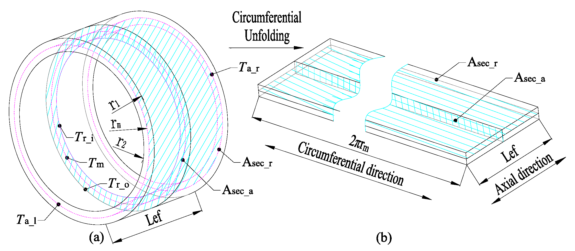
Based on three types of thermal network unit, namely “H”, “+” and “I” type, the exponential decay function method and the exponential decay iteration method are deduced. The two methods are used to calculate the first-order LPTN. For a given constant power loss and total heat flux, the bigger the convection heat transfer coefficient value, the lower the steady-state temperature of the yoke iron core. The geometry parameters of a general hollow cylinder and its unfolded brick are given in Figure 1. It also considers different heat source locations relative to the center of mass [14]. The definitions of the parameters are given in Figure 1.

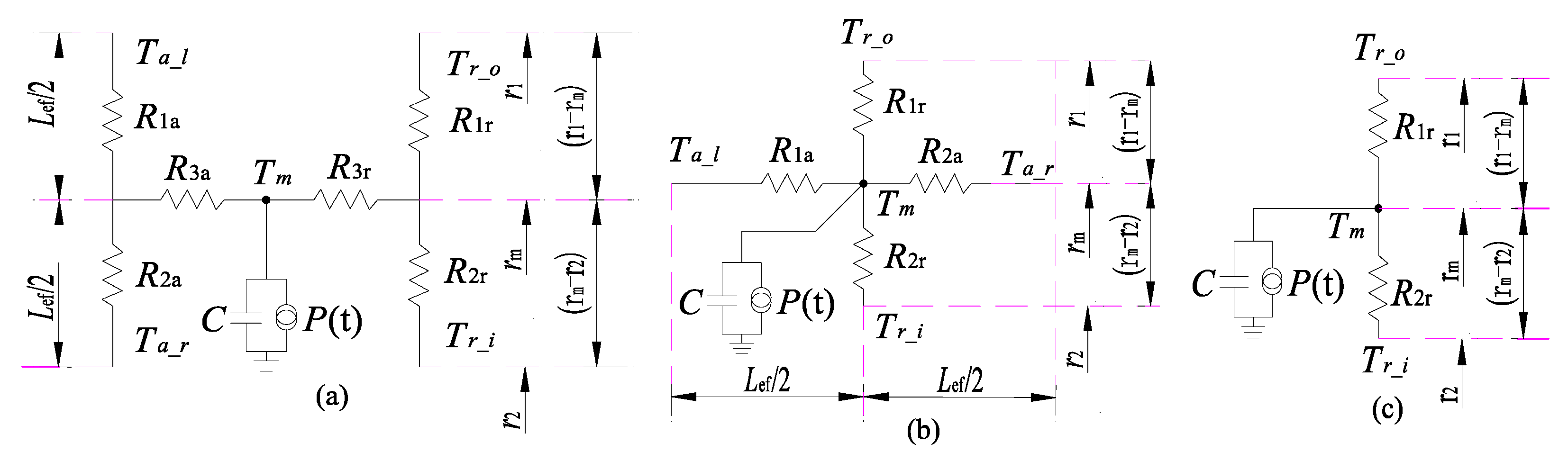
Thermal network units of “H” type, “+” type and “I” type are adapted to the geometric shape of torus and brick. Thermal network units of “H” type, “+” type and “I” type define thermal resistance, thermal capacitance, and power loss, which are shown in Figure 2a–c, respectively.

Heat resistance R_cond is the inverse of heat conductance G_cond, which is given by [14]

$$R_{cond}=\frac{l}{\lambda A_{sec}},G_{cond}=\frac{1}{R_{cond}}$$

(1)

where l is the length in the direction of thermal conductivity (m), λ is the coefficient of thermal conduction (W/m·K) and A_sec is the cross-section perpendicular to the direction of thermal conduction (m²).

The equivalent thermal conductance G_mat1,2 of two kinds of materials with or without assembly clearance is considered as follows [14].

$$\{\begin{array}{l}{G}_{mat1,2}=\frac{1}{1/G_{mat1}+1/G_{air}+1/G_{mat2}}\\ G_{mat1,2}=\frac{1}{1/G_{mat1}+1/G_{mat2}}\end{array}$$

(2)

where G_air is the thermal conductance of air.

2.1. Thermal Network Unit of “H” Type

The thermal network unit of “H” type includes radial and axial thermal resistance (R_1r, R_2r, R_1a, R_2a), which are given in Figure 2a and

Table 1. Thermal resistance definition of “H” type [15,16,17,18,19].

Radial R1r, R2r, R3r	Axial R1a, R2a, R3a
$R_{1r}=\frac{1}{4\pi {\lambda }_{r}l}\left(1-\frac{2r_2^2\ln \left(r_1/r_2\right)}{r_1^2-r_2^2}\right)\hspace{1em}\hspace{1em}\hspace{1em}\hspace{1em}{R}_{1a}=\frac{l}{2\pi {\lambda }_a(r_1^2-r_2^2)}$
$R_{2r}=\frac{1}{4\pi {\lambda }_{r}l}\left(\frac{2r_1^2\ln \left(r_1/r_2\right)}{r_1^2-r_2^2}-1\right)\hspace{1em}\hspace{1em}\hspace{1em}\hspace{1em}{R}_{2a}=\frac{l}{2\pi {\lambda }_a\left(r_1^2-r_2^2\right)}$
$R_{3r}=-\frac{\left(r_1^2+r_2^2\right)}{8\pi {\lambda }_{r}l\left(r_1^2-r_2^2\right)}+\frac{r_1^2{r}_2^2\ln \left(r_1/r_2\right)}{2\pi {\lambda }_{r}l{\left(r_1^2-r_2^2\right)}^2}\hspace{1em}\hspace{1em}\hspace{1em}\hspace{1em}{R}_{3a}=\frac{-l}{6\pi {\lambda }_a\left(r_1^2-r_2^2\right)}$

.

2.2. Thermal Network Unit of “+” Type

The thermal network unit definition of “+” type includes radial and axial thermal resistance (R_1r, R_2r, R_1a, R_2a), as shown in Figure 2b. We assume here that heat source location coincides with a center of mass. Here, middle radius is given as r_m = (r₁ + r₂)/2. Its thermal resistance is calculated in

Table 2. Thermal resistance definition of “+” type.

Radial R1r, R2r	Axial R1a, R2a
$R_{1r}=R_{2r}=\frac{\left(r_1-r_2\right)}{4{\lambda }_r\pi r_{m}l}\hspace{1em}\hspace{1em}\hspace{1em}\hspace{1em}{R}_{1a}=R_{2a}=\frac{l}{2{\lambda }_a\left(r_1^2-r_2^2\right)}$

.

2.3. Thermal Network Unit of “I” Type

The thermal network unit definition of “I” type only includes radial thermal resistance, which are R_1r and R_2r, as given in Figure 2c and

Table 3. Thermal resistance definition of “I” type [6].

Radial R1r	Radial R2r
$R_{1r}=\frac{1}{2\pi {\lambda }_{r}l}\ln \left(\frac{r_m}{r_2}\right)\hspace{1em}\hspace{1em}\hspace{1em}\hspace{1em}{R}_{2r}=\frac{1}{2\pi {\lambda }_{r}l}\ln \left(\frac{r_1}{r_m}\right)$

.

Take stator yoke iron core as example; its dimensions are Φ_{yo_o}×Φ_{yo_i}×L_ef: 208 × 178 × 120 (mm). According to theoretical equations of thermal resistance unit in Table 1, Table 2 and Table 3, the calculation results of three kinds of thermal network unit are given in

Table 4. Thermal resistance results with three methods.

Thermal Resistance	Radial Rr (K/W)		Axial Ra (K/W)
“H” type	R1r	0.0023	R1a	1.466
	R2r	0.0022	R2a	1.466
	R3r	−7.63 × 10−4,	R3a	−0.489
“+” type	R1r	0.0023	R1a	1.466
	R2r	0.0023	R2a	1.466
“I” type	R1r	0.0024	—	—
	R2r	0.0022	—	—

.

Due to radial thermal conductivity λ_r = 45 W/(m·K) being much larger than axial thermal conductivity λ_a = 4.5 W/(m·K), radial resistance R_r is much less than axial resistance R_a. For the thermal network unit of the stator iron core and rotor iron core, heat transfer in the axial direction may be negligible. Therefore, we can approximately substitute “I” type for “H” type and “+” type, which can obviously reduce matrix size and computational burden.

3. Transient Thermal Network Method of First Order

In this section, a multi-node LPTN model of IPMSM is established based on the “+” type of thermal network unit. A heat capacity matrix, thermal conductivity matrix and node loss matrix of LPTN are established. A first-order, non-homogeneous linear differential equation is solved through discretization, and the temperature rise curves of each node changing with time step iteration are obtained. Operating conditions considering copper resistivity variation are analyzed based on the LPTN.

3.1. First-Order Transient LPTN Theory

Thermal flux q_sec (heat flow intensity) through the unit section area (W/m²) is given as

$$q_{sec}=\lambda \frac{\partial T}{\partial d}=h\left(T_{act}-T_0\right)$$

(3)

where h is the convection heat transfer coefficient (W/m²·°C), T_act is the actual temperature of the steady state (°C), T₀ is ambient temperature(°C) and d is thickness in the direction of heat conduction (m).

Thermal flux q_sec through cross-sectional area A_sec is a constant. It eventually reaches the steady-state temperature (generated heat equals dissipated heat) by convection, as shown in

$$P_{loss}\left(t\right)=h\left( T_{act}\left(t\right)-T_0 \right)A_{sec}=q{A}_{sec}$$

(4)

where A_sec is the outer circumferential surface area of the stator yoke iron core (m²).

The temperature rise T(t) is described by an exponential decay function as below.

$$T\left(t\right)=P_{loss}\left(t\right)R_{eq}\left(1-e^{-t/\left(R_{eq}{C}_{eq}\right)}\right)$$

(5)

$$T_{act}\left(t\right)=T\left(t\right)+T_0$$

(6)

where R_eq is equivalent thermal resistance (R_eq = R_cond + R_conv) and C_eq is equivalent thermal capacity (C_eq = C).

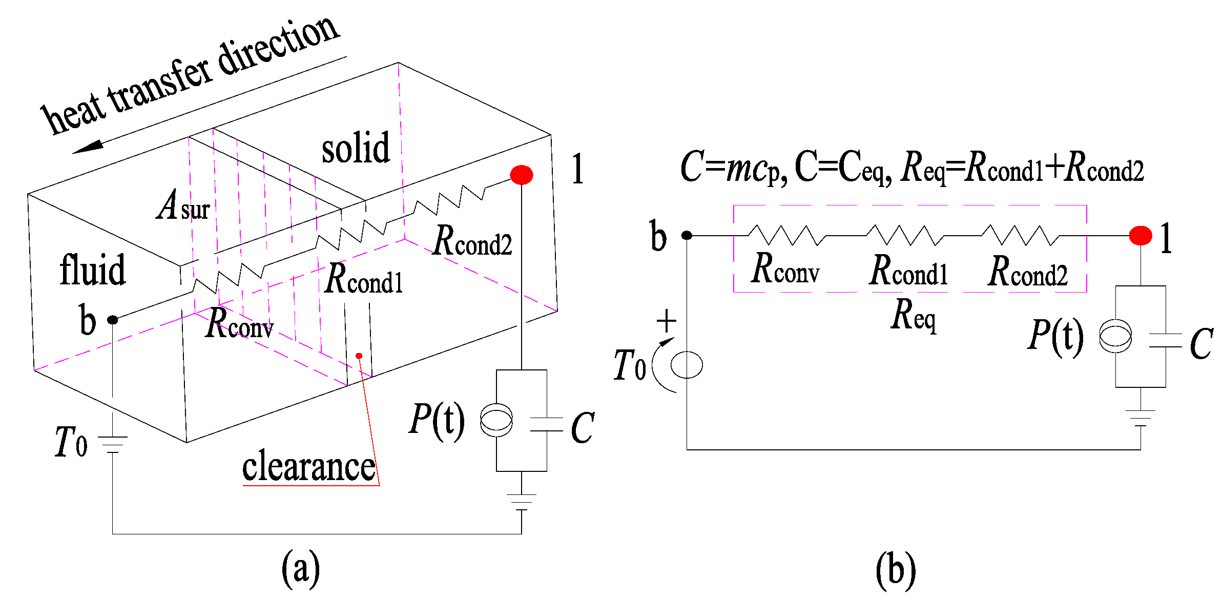
It is assumed that the stator yoke core generates a continuous power loss of P_{sta_yo} = 410 W (heat source P_{sta_yo} is constant) and is dissipated by a single end face. If the LPTN unit is composed of a single heat source, its thermal resistance and thermal capacity are as shown in Figure 3a. The heat is transferred in a single direction, and its corresponding first thermal network is defined in Figure 3b. The heat transfer process is defined from one end face to another, which leads to a temperature rise (T_act-T₀) in the yoke iron core. Similarly, the first-order model and its thermal network with air clearance are given in Figure 4a,b.

If an end face has convection with the ambient air, thermal-convection resistance R_conv should be connected with thermal-conduction resistance R_cond in series. The smaller the convective thermal resistance, the stronger the convective heat transfer ability; the range covers air cooling to water cooling. The more heat is dissipated to the ambient air, the lower the temperature rise of the cuboid itself. If there is no convective thermal resistance R_conv to the ambient air, the boundary of the cuboid is an isothermal boundary, which reaches the limits of the thermal convection capacity.

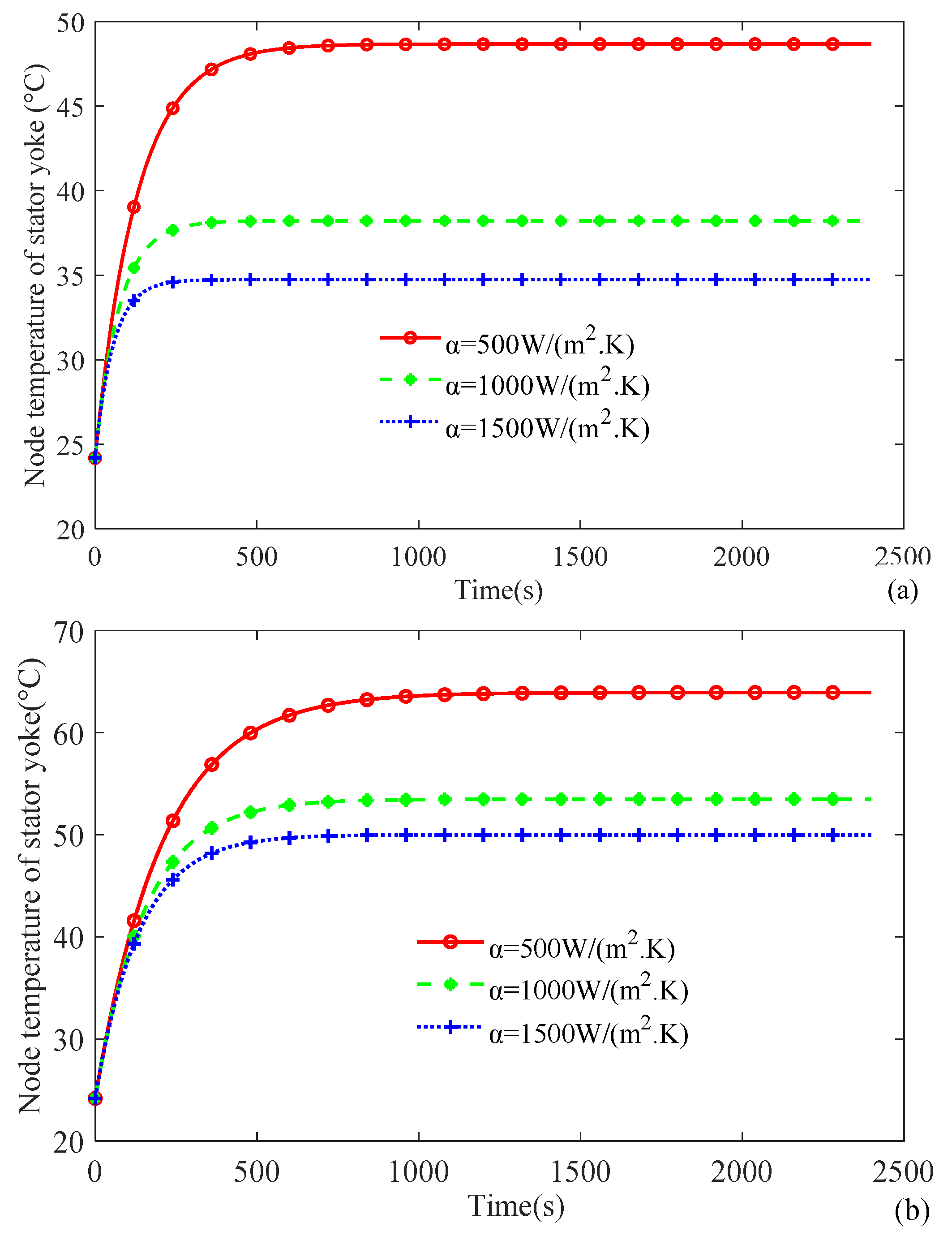
When the convective heat transfer coefficient α takes different values with or without assembly clearance (h_ac = 0.03 mm), the transient temperature curve with time is obtained, as shown in Figure 5. For the given stator yoke loss (P_{sta_yo} = 410 W), the time of reaching the node steady temperature depends on the cooling ability of heat dissipation to the ambient air and thermal resistance along the heat transfer path. In other words, the increase in heat transfer convection coefficient α and the decrease in assembly clearance help to reduce the node temperature rise and shorten the time to reach the steady state (about 2500 s).

3.2. Multi-Order LPTN Theory

The transient temperature rise can be solved by the following differential equation.

$$Q\left(t\right)=\rho Vc\Delta T=C\Delta T=\left[P\left(t\right)-GT\left(t\right)\right]\Delta t$$

(7)

$$\dot{T}\left(t\right)»\frac{T\left(t+\Delta t\right)-T\left(t\right)}{\Delta t}=C^{-1}\left[P-GT\left(t\right)\right]$$

(8)

where the part density ρ, part volume V, part mass m, specific heat capacity c and thermal capacity C are nxn diagonal matrixes, respectively. ΔT is the column vector of the temperature difference value. Q(t) is the quantity of heat and P(t) is the power loss of part node (W). G is the nxn thermal conductivity symmetric matrix (W/°C). T is the column vector of temperature rise (°C).

If the change in resistivity caused by temperature rise is considered, the loss matrix P(t) should update in every time step. The change rate of the temperature rise matrix can be obtained by solving the first-order inhomogeneous differential equation T(t).

$$\dot{T}\left(t\right)=C^{-1}P\left(t\right)-C^{-1}GT\left(t\right)$$

(9)

The general solution of the first-order inhomogeneous differential equation is the sum of the general solution of the corresponding homogeneous linear equation and a particular solution of the inhomogeneous linear equation, where the constant term of the general solution of the homogeneous linear equation is C_con = T(t₀).

$$T\left(t\right)=T\left(t_0\right)e^{-C^{-1}G\left(t-t_0\right)}+{\displaystyle {\int }_{t_0}^t{e}^{-C^{-1}G\left(t-\tau \right)}d\tau }{C}^{-1}P\left(t\right)$$

(10)

The continuous equation in (10) is discretized with (11). At time (n + 1)Δt and nΔt, the temperature relation between T[(n + 1) Δt] and T(nΔt) is given by

$$T\left[\left(n+1\right)\Delta t\right]=e^{-C^{-1}G\Delta t}T\left(n\Delta t\right)-G^{-1}C\left(e^{-C^{-1}G\Delta t}-I\right)C^{-1}P\left(n\Delta t\right),n=0,1,2\cdots$$

(11)

The actual temperature T_act(nΔt) of each node is the sum of the ambient temperature T_amb and the node temperature rise T(nΔt).

$$T_{act}\left(n\Delta t\right)=T_{amb}+T\left(n\Delta t\right)$$

(12)

When the convergence criterion (T(n + 1) Δt − T(n) Δt)/T(n + 1)Δt < ε is satisfied, the iteration process is terminated. We assume n_maxΔt−τ is equal to u. The steady-state temperature rise calculation is simplified as

$$T\left(n_{max}\Delta t\right)={\displaystyle {\int }_{t_0}^{n_{max}\Delta t}{e}^{-C^{-1}G\left(n_{max}\Delta t-\tau \right)}d\tau }{C}^{-1}P\left(t\right)=G^{-1}P\left(t\right)$$

(13)

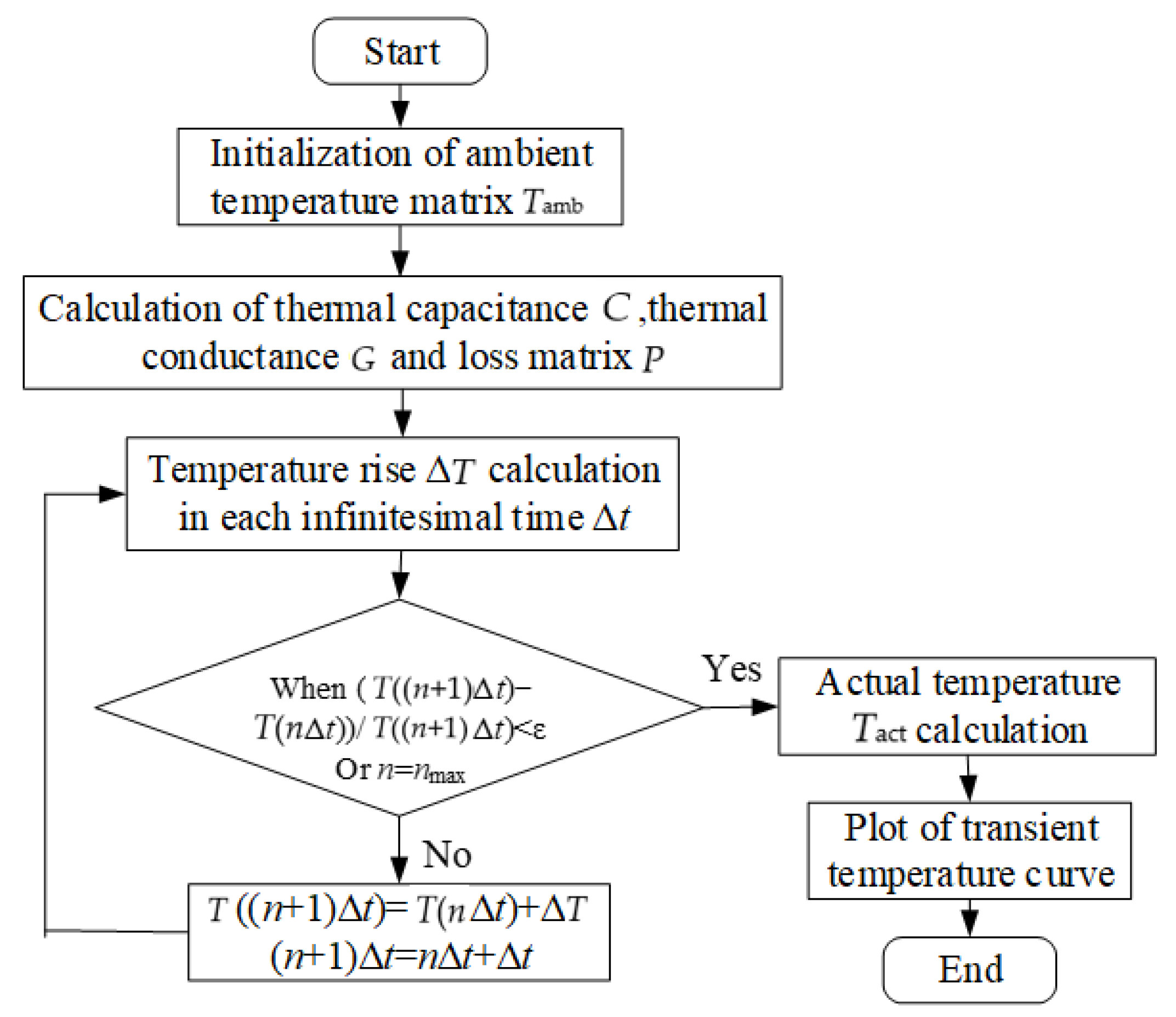
According to Equations (7)–(13), the flow chart of the transient temperature rise calculation of IPMSM is given in Figure 6. The flow chart also describes the change process from ambient temperature T_amb to steady-state temperature T_max.

4. Transient Thermal Network of IPMSM

A half 40 kW IPMSM model and LPTN of temperature node distribution are built for its axial symmetry in Figure 7a,b in this paper. For the transient thermal network model, the IPMSM model is divided into the following 14 parts: (1) outer shell, (2) inner shell, (3) stator yoke, (4) stator tooth, (5) slotted winding, (6) end winding, (7) rotor shoe, (8) PM, (9) rotor yoke, (10) shaft, (11) end cap, (12) bearing, (13)–(14) inner air, (a), (c), (d) ambient air and (b) water.

Main heat generated by losses is taken away by circulating coolant in the shell. Therefore, the shell is divided into the outer shell (1# node) and the inner shell (2# node) considering heat convection. Due to the flux density difference between the stator tooth (3# node) and the stator yoke (4# node), losses of stator tooth and stator yoke are considered separately. Similarly, rotor iron loss falls into the rotor shoe (7# node) loss and the rotor yoke (9# node) loss. The winding is divided into slotting winding (5# node) and end windings (6# node). The end cap (11# node) and the shaft (10# node) are regarded as single non-heat source nodes. The wind friction loss is exerted on the rotor shoe (7# node). Loss values for the heat generation are applied to heat source nodes of the IPMSM.

For the non-heat source nodes, thermal capacity and thermal resistance connected with adjacent nodes are considered. For the heat source nodes, thermal capacity, power loss and thermal resistance are considered. The transient thermal network model is given in detail in Figure 7b.

The main parameters of IPMSM are given in

Table 5. IPMSM Dimensions and Parameters.

Parameter	Value
Bus voltage Udc [V]	360	Number of turns per coil Ns	10
Rated power Pn [kW]	40	Length of air gap δ [mm]	1.5
Rated speed n [rpm]	4000	PM thickness hpm [mm]	6
Inner diameter of stator iron Dsi [mm]	150	Number of stator slots Q	48
Outer diameter of stator iron Dso [mm]	208	Number of pole pairs p	4
Length of stator iron Lef [mm]	160	Winding connection	Y
Number of parallel branches a	2	Coolant flow speed V [L/min]	8

. Loss values for the heat generation are applied to the IPMSM parts. Loss values at rated load and node number are also given in

Table 6. Loss value of IPMSM parts.

Parameter	Symbol	Value	No.
Stator yoke loss [W]	PFej	410	3
Stator tooth loss [W]	PFet	282	4
Slot winding loss [W]	PCu1	810	5
End winding loss [W]	PCu2	651	6
Rotor pole shoe loss [W]	Pros	20	7
PM eddy loss [W]	Ppm	38	8
Rotor yoke iron loss [W]	Proy	45	9
Bearing loss [W]	Pbe	0.11	12
Air friction loss [W]	Pair	20	13

Loss values at 40 kW power and speed of 4000 rpm.

for the volume heat generation of IPMSM parts.

5. Load Case Analysis and Experiment

Transient temperature rise considering actual copper resistivity and intermittent condition is analyzed in this section.

5.1. Consant Load Considering Copper Resistivity

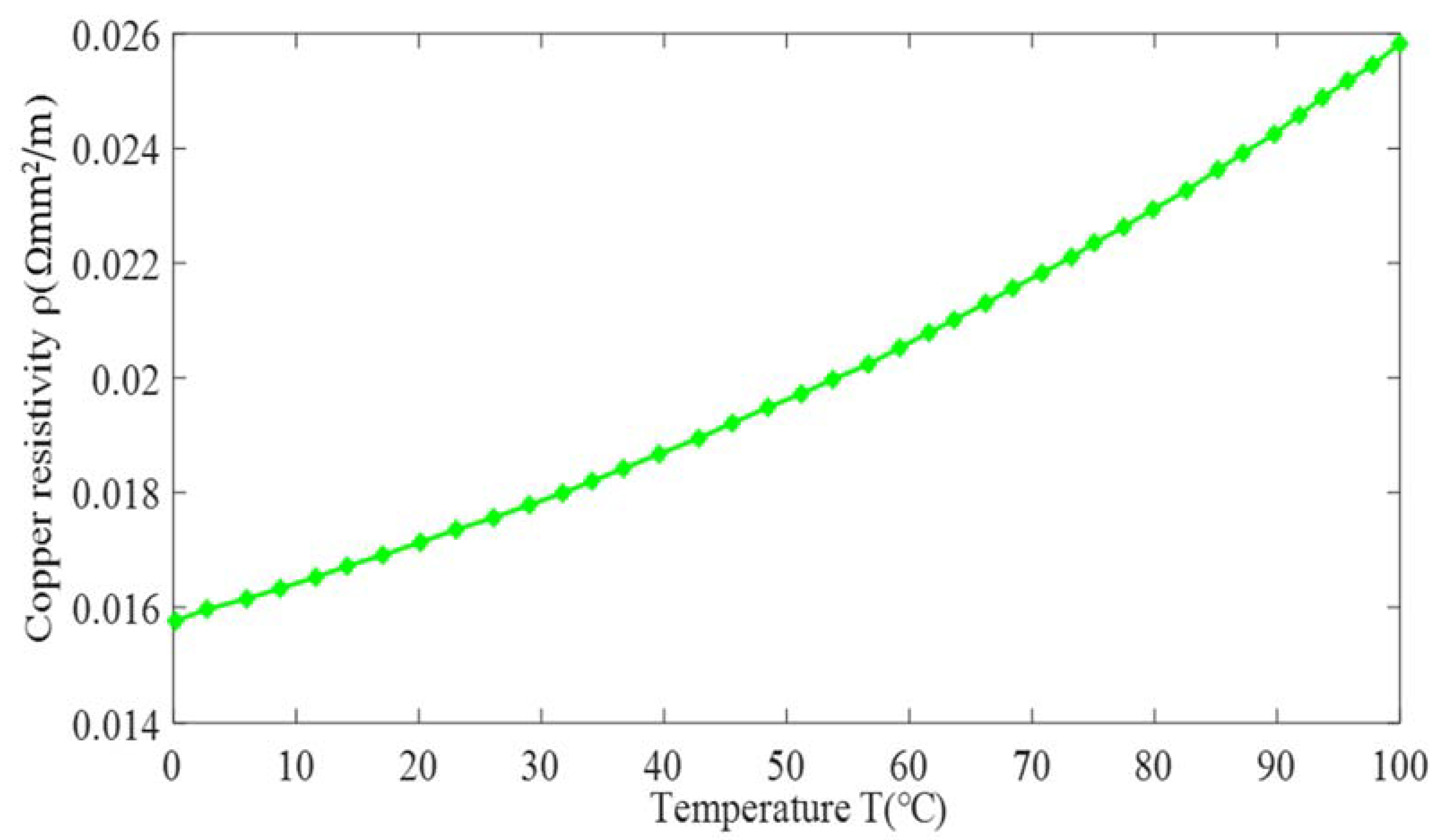
Winding copper loss P_Cu of two groups of phases, phase resistance R and copper resistivity ρ considering electrical resistivity variation with temperature are defined as:

$$\{\begin{array}{l}{P}_{Cu}=m{I}^2{R}_0\left(1+\alpha T\right)=m{I}^2{R}_{20}\left(1+\alpha \left(T-20\right)\right)\\ R={\rho }_0\left(1+\alpha T\right)\frac{L}{S}={\rho }_{20}\left(1+\alpha \left(T-20\right)\right)\frac{L}{S}\\ \rho ={\rho }_0\left(1+\alpha T\right)={\rho }_{20}\left(1+\alpha \left(T-20\right)\right)\end{array}$$

(14)

where T₀ is ambient temperature (°C), ρ₀ is the electrical resistivity of copper at 0 °C (ρ₀ = 0.0165 Ω mm²/m), ρ₂₀ is the electrical resistivity of copper at 20 °C (ρ₂₀ = 0.0176 Ω mm²/m), and α is the temperature coefficient of copper (α = 0.0039/°C). The winding copper resistivity ρ increases slightly with the increase in temperature T as shown in Figure 8.

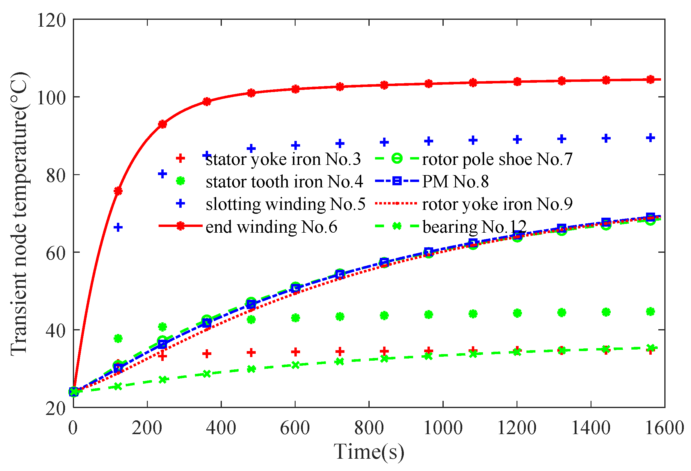
Based on the LPTN of IPMSM in Figure 7b and Equations (7)–(13), transient node temperature curves of the main heat sources are given in Figure 9.

First-order, second-order, and third-order exponential decay functions are used to predict the transient winding temperature for two operating points, which are given as

$$\{\begin{array}{l}{y}_{1\mathrm{t}\mathrm{h}}\left(x\right)=A_1{e}^{-x/t_1}+y_0\\ y_{2\mathrm{t}\mathrm{h}}\left(x\right)=A_1{e}^{-x/t_1}+A_2{e}^{-x/t_2}+y_0\\ y_{3\mathrm{t}\mathrm{h}}\left(x\right)=A_1{e}^{-x/t_1}+A_2{e}^{-x/t_2}+A_3{e}^{-x/t_3}+y_0\end{array}$$

(15)

where y₀ is the offset distance; A₁~A₃ are amplitude; t₁~t₃ are the decay constant.

The parameters of three kinds of exponential decay functions are calculated by origin as shown in

Table 7. Loss value of IPMSM parts.

Order	Sym	Value	Sym	Value
	3000 rpm—40 kW		6000 rpm—40 kW
1st	y0	106.69	y0	80.18
	A1	−78.64	A1	−49.16
	t1	190.44	t1	300.55
2nd	y0	109	y0	81.3
	A1	−38.21	A1	−12.23
	t1	372.11	t1	29.82
	A2	−46.26	A2	−44.03
	t2	100.99	t2	371.06
3rd	y0	109	y0	81.3
	A1	−23.13	A1	−12.23
	t1	101.01	t1	29.82
	A2	−23.13	A2	−21.95
	t2	100.97	t2	371.08
	A3	−38.21	A3	−22.08
	t3	372.11	t3	371.05

.

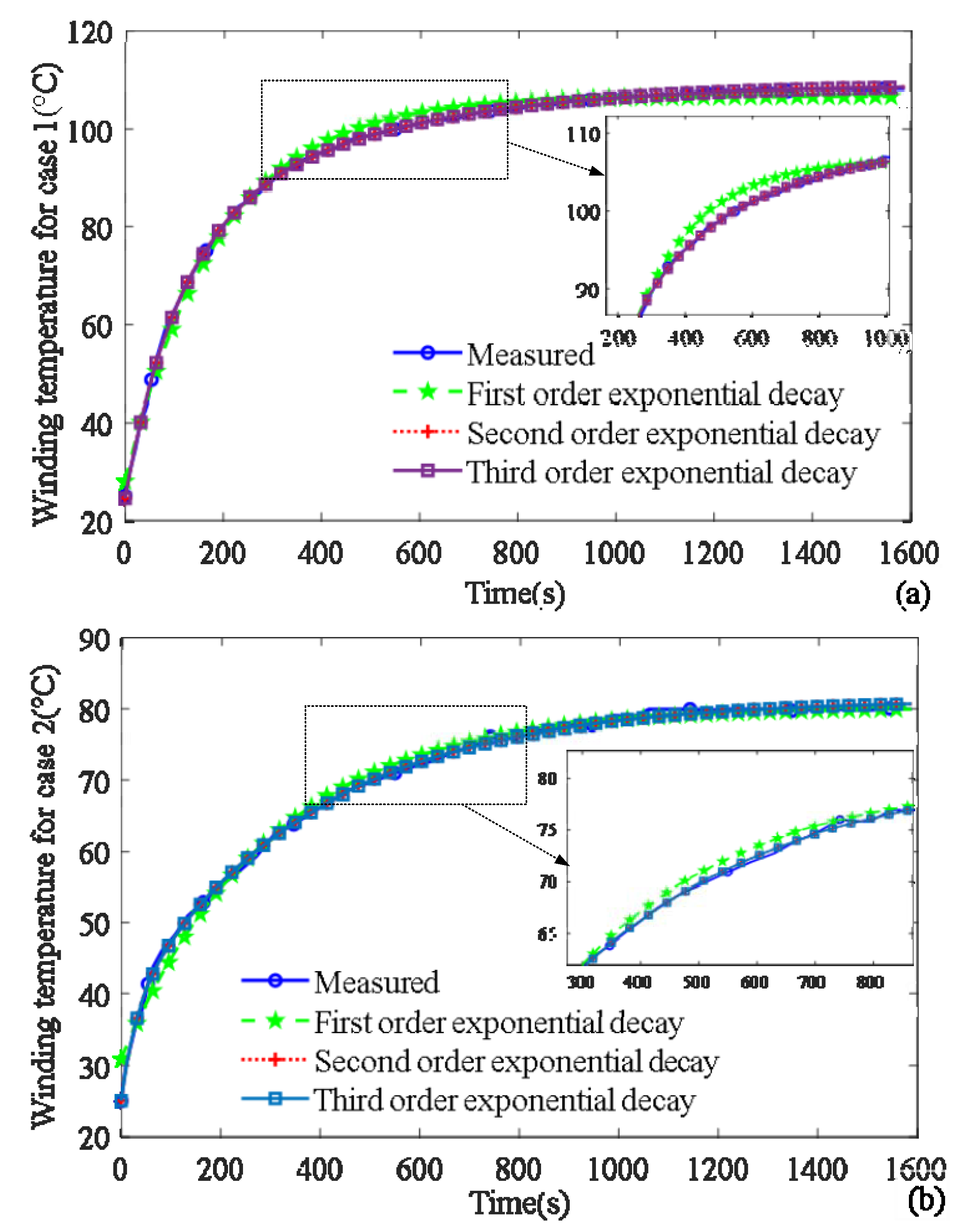
Comparison between the measured transient winding temperature and nonlinear exponential fit curves are given for two operating points. The first operating case in Figure 10a is line voltage U_ab = 196.6 V, phase current I_a = 203.1 A, speed n = 3000 rpm and P_n = 40 kW. The second operating case in Figure 10b is line voltage U_ab = 245.6 V, phase current I_a = 119.2 A, speed n = 6000 rpm and P_n = 40 kW. Winding temperature reaches the steady state after 1600 s, which benefits from the excellent heat dissipation of the water cooling. We can see from Figure 10 that the exponential decay fit function of the second order and the third order has higher accuracy than that of the first order.

5.2. Rectangular Wave Load

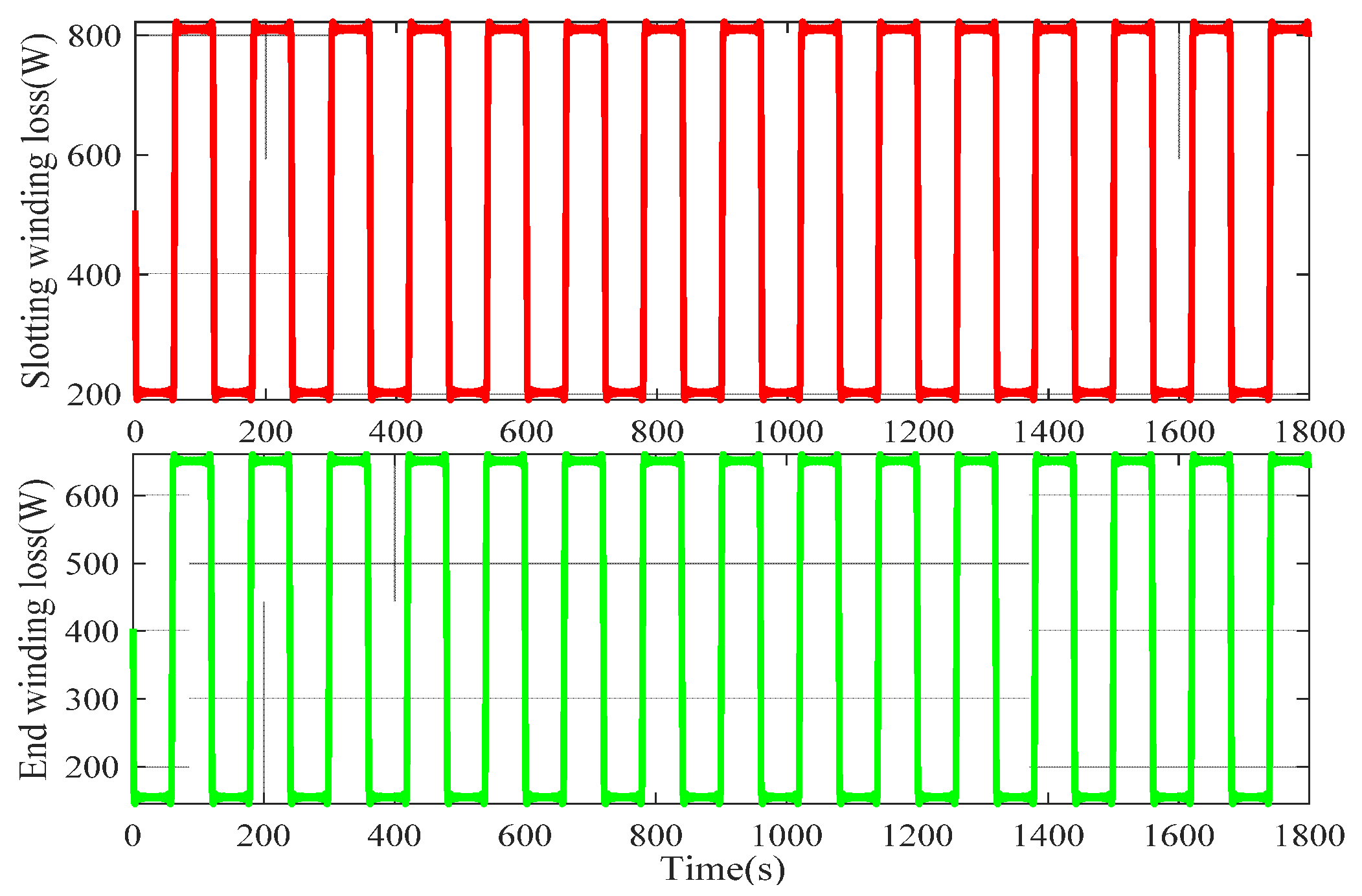
The copper loss curve of the rectangular periodic wave is discontinuous at the orthogonal turning point. Therefore, copper loss curve data expressed by Fourier series are loaded discretely. Slotting winding loss and end winding loss are applied to corresponding objects in the form of Fourier series. We set a period of 120 s and run 15 cycles. Winding loss is given as

$$\{\begin{array}{l}{P}_{\mathrm{slo}\_\mathrm{win}}\left(t\right)={\alpha }_{\mathrm{dt}}\left(A_{\mathrm{slo}\_\mathrm{win}1}-A_{\mathrm{slo}\_\mathrm{win}2}\right)+A_{\mathrm{slo}\_\mathrm{win}2}\\ \hspace{1em}\hspace{1em}\hspace{1em}\hspace{1em}-{\displaystyle \sum _{n=1}^{\infty }\frac{1}{n\pi }\left(\begin{array}{l}2\left(A_{\mathrm{slo}\_\mathrm{win}1}-A_{\mathrm{slo}\_\mathrm{win}2}\right)\cdot \\ \sin \left({\alpha }_{\mathrm{dt}}n\pi \right)\cos \left(n\omega t-{\alpha }_{\mathrm{dt}}n\pi \right)\end{array}\right)}\\ P_{\mathrm{end}\_\mathrm{win}}\left(t\right)={\alpha }_{\mathrm{dt}}\left(A_{\mathrm{end}\_\mathrm{win}1}-A_{\mathrm{end}\_\mathrm{win}2}\right)+A_{\mathrm{end}\_\mathrm{win}2}\\ \hspace{1em}\hspace{1em}\hspace{1em}\hspace{1em}-{\displaystyle \sum _{n=1}^{\infty }\frac{1}{n\pi }\left(\begin{array}{l}2\left(A_{\mathrm{end}\_\mathrm{win}1}-A_{\mathrm{end}\_\mathrm{win}2}\right)\cdot \\ \sin \left({\alpha }_{\mathrm{dt}}n\pi \right)\cos \left(n\omega t-{\alpha }_{\mathrm{dt}}n\pi \right)\end{array}\right)}\end{array}$$

(16)

where α_dt is the duty cycle (here α_dt = 0.5), A_{slo_win1} and A_{slo_win2} are the upper and lower values of slotting winding loss (W), A_{end_win1}, A_{end_win2} are the upper and lower values of end winding loss (W), respectively, and ω is the angular frequency (rad/s).

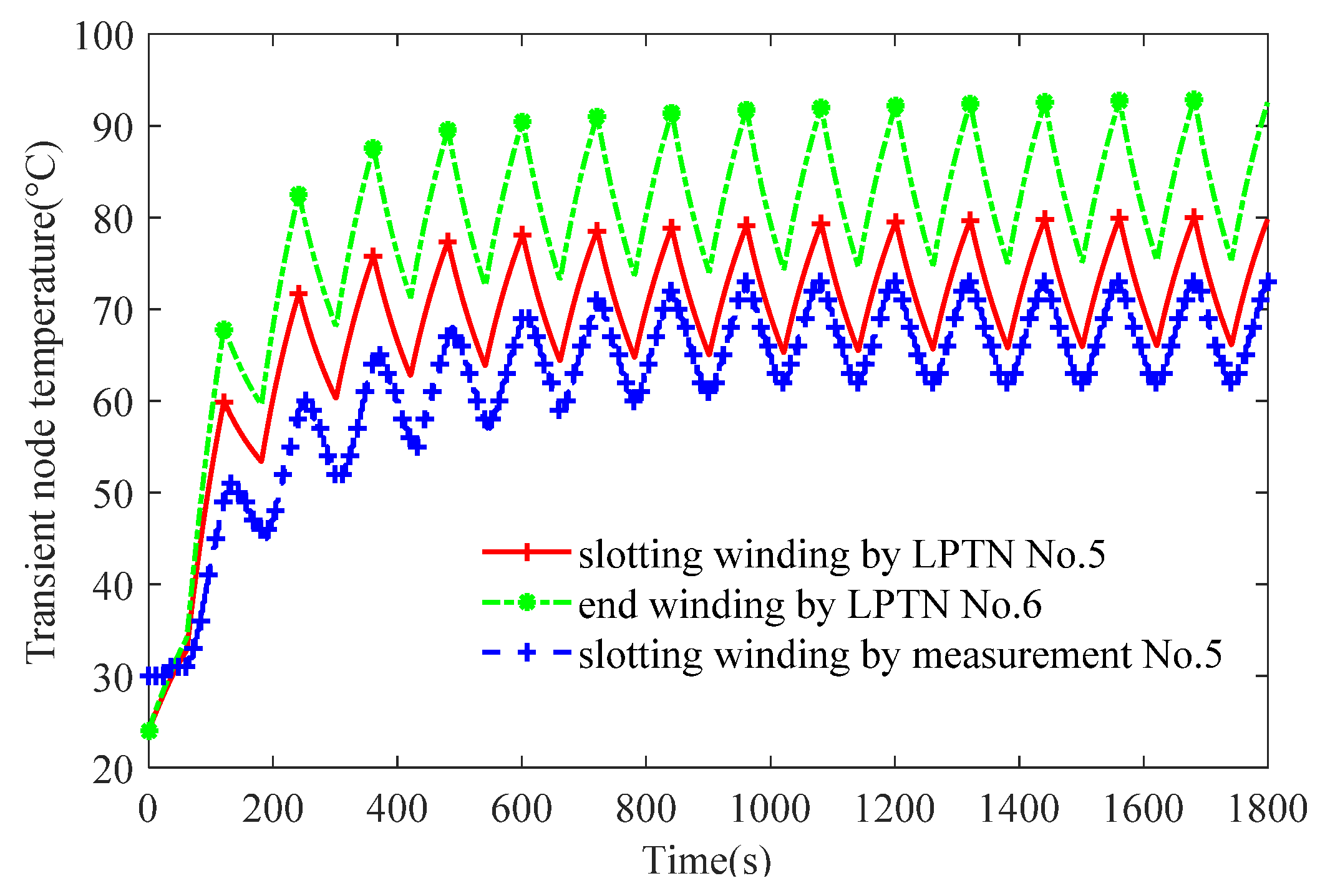
Rectangular wave loss of slotting winding and end winding is given in Figure 11. A rectangular periodic step torque from light load to heavy load is simulated, which leads to the change of winding loss (A_{slo_win1} = 810 W, A_{slo_win2} = 203 W, A_{end_win1} = 651 W, A_{end_win2} = 155 W). The thermal source matrix is updated at every time step and transient temperature curves of slotting winding and end winding are given in Figure 12. We can find that the calculation result of LPTN agrees well with the outcome of the experiment. For the slotting winding at the steady state, there is about an 8 °C error between the measurement value and the LPTN value. The reason for the higher value is that the value of thermal resistance or winding loss may be high for single node modeling.

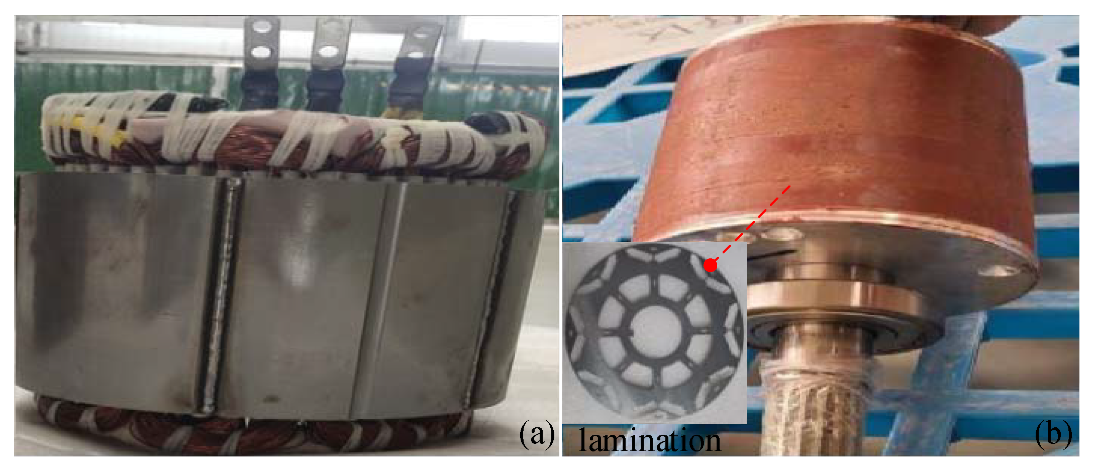
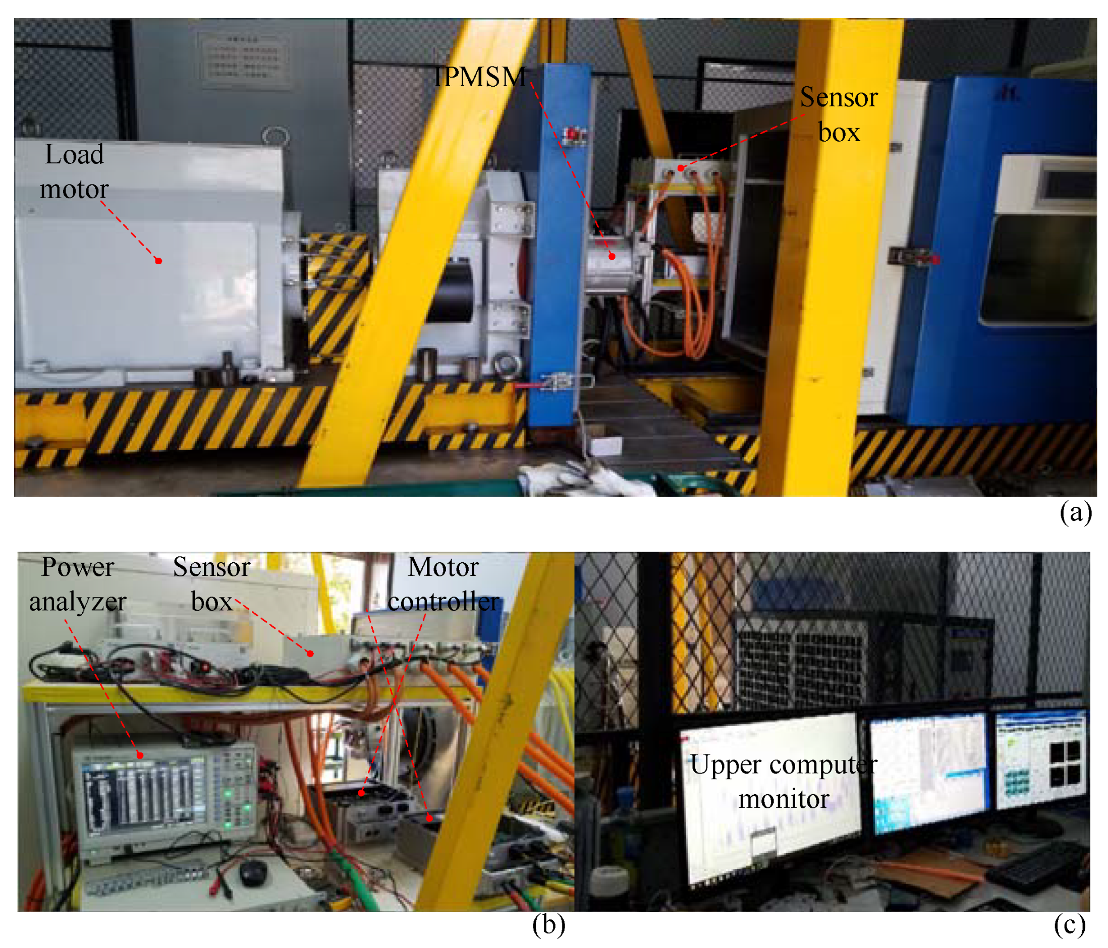
In order to verify the LPTN model, the prototype of 48-slot/8-pole IPMSM with “V” type rotor and ISDW stator is designed and manufactured. The stator and rotor are shown in Figure 13. A load test platform is established to validate its temperature rise and output characteristics, as shown in Figure 14.

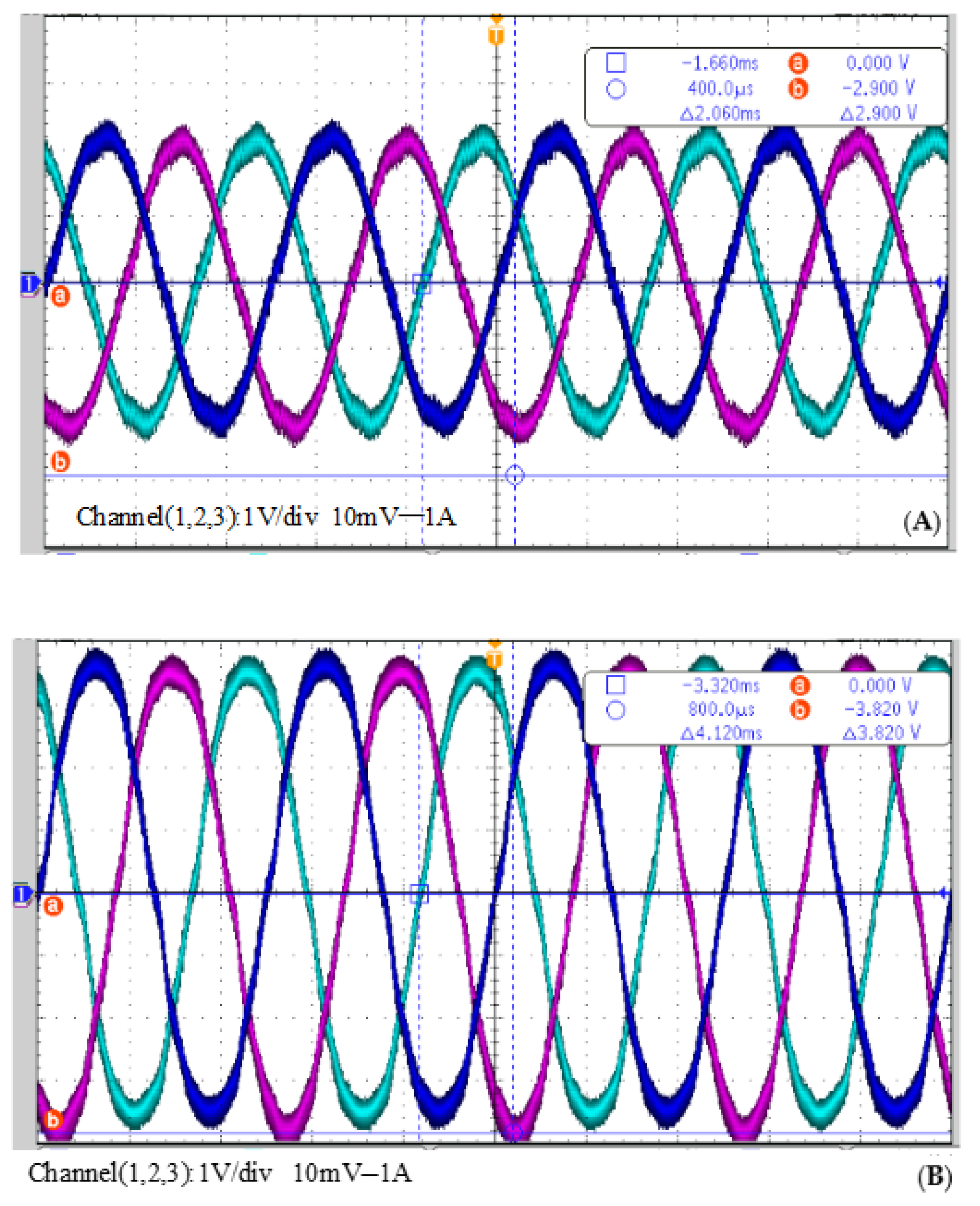
The measured phase current wave using three AC current clamps under rated load conditions is shown in Figure 15A, whose peak value reaches 232 A. The phase current under overload conditions is obtained in Figure 15B, whose peak value reaches 382 A.

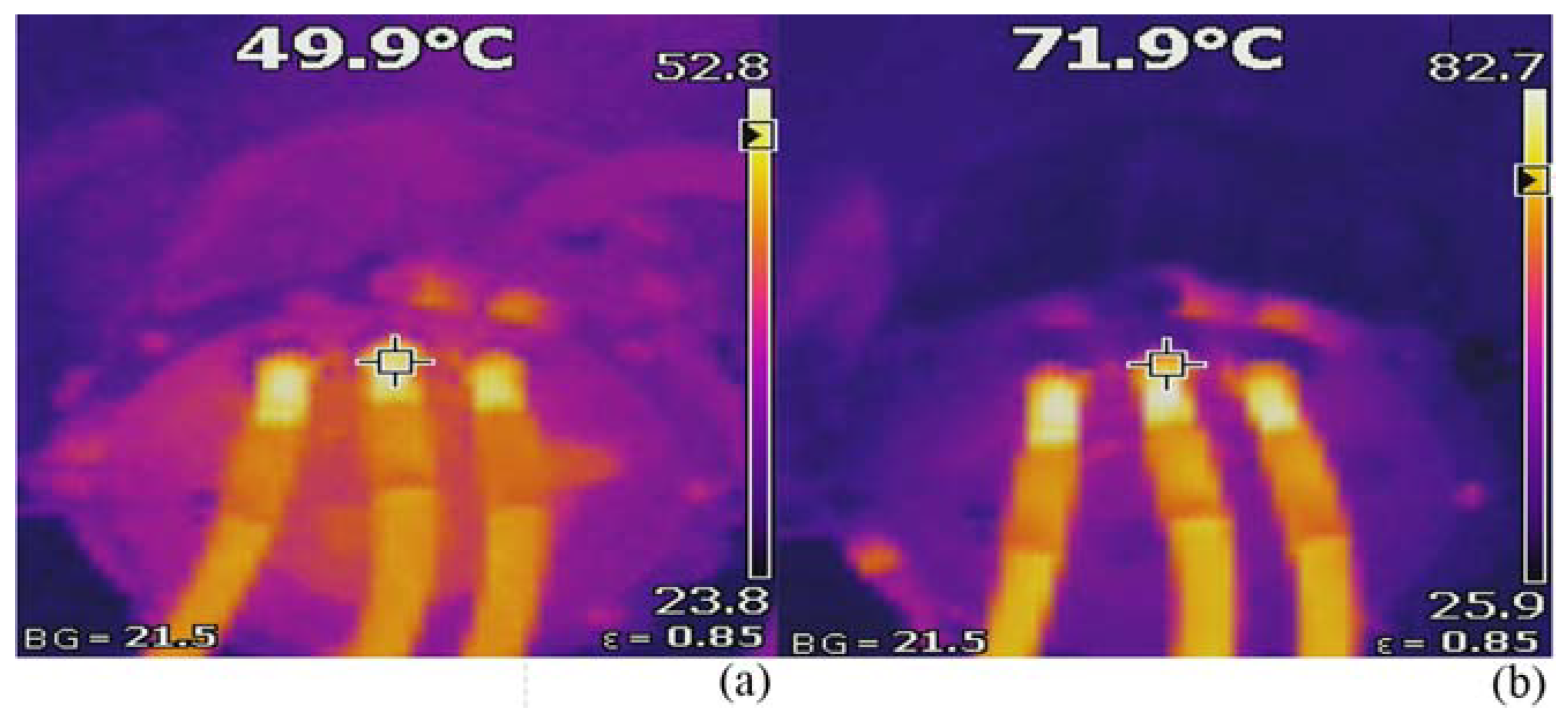
The temperature of the IPMSM parts is measured by thermocouple PTC100 and a FLUKE infrared imaging device. Thermocouple temperature sensors PTC100 are inserted into slotted windings for measuring the temperature of the slotted winding. The outer surface temperature of the IPMSM is measured by using a FLUKE infrared imaging device in Figure 16.

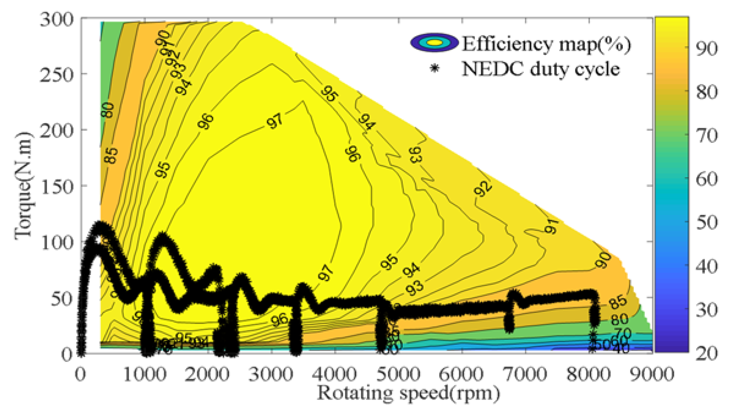
The measured IPMSM efficiency versus different load torques at 3000 rpm and 6000 rpm are given in Figure 17. We found that efficiency is higher at a rated speed of 3000 rpm. Due to a large copper loss and iron loss in the field-weakening region, efficiency is relatively low. A measured IPMSM efficiency map including constant torque and constant power operating regions is given in Figure 18. The operating point of the NEDC duty cycle is also obtained by the test platform as shown in Figure 18. We found that the maximum efficiency of IPMSM reaches about 97%; however, the relatively low efficiency in the constant power operation region ranges from 80% to 87% for the NEDC duty cycle.

6. Conclusions

The method of the first-order LPTN is deduced by solving the non-homogeneous linear differential equation. The results show that the heat transfer coefficient of fluid and thickness of air gap layer are the main influencing factors for reaching a steady temperature. The larger the heat transfer coefficient of fluid is, the lower the steady node temperature is. The smaller the air layer thickness is, the lower the steady node temperature is.

Furthermore, the multi-order LPTN theory is deduced based on the extension of first-order transient LPTN. For the constant load and rectangular periodic load, the transient node temperatures of IPMSM are obtained by modeling transient LPTN and solving the non-homogeneous linear differential equation. Compared with the experimental data, exponential decay fit function of the second order and the third order has higher accuracy than that of the first order, which can serve as an alternative to full-order thermal networks.

The temperature rise experiment platform including IPMSM manufacture is established to validate the above-mentioned method using a FLUKE infrared thermal imager and thermocouple PTC100. Load current and efficiency maps are obtained using the dynamometer platform. The load experiment shows that the transient LPTN of the IPMSM can accurately predict node temperature variation.