Formation of Characteristic Polynomials on the Basis of Fractional Powers j of Dynamic Systems and Stability Problems of Such Systems

Abstract

The article presents the creation of characteristic polynomials on the basis of fractional powers j of dynamic systems and problems related to the determination of the stability intervals of such systems.

1. Introduction

The implementation of automatic control systems (ACS) with the required static and dynamic characteristics is possible if, first of all, the condition of such system stability is met. In the case of ACS analysis, which is given by differential equations with integer derivatives, the methods for studying stability are well known. This investigation used algebraic or frequency stability criteria. The Mikhailov’s frequency criterion has become especially widespread for engineering studies of ACS stability. That is due to its simplicity and clarity. The proof of this method is based on the analysis of the change in the position of the vectors (jω-p_i) on the complex plane when the poles’ locations of the transfer function are in the right half-plane (system is not stable) and left half-plane (system is stable). The Mikhailov’s criterion of stability is formulated on the base of the requirement of the signal frequency changing ω within all permissible limits. It is necessary to justify using the frequency criteria, in particular Mikhailov’s criteria, to analyze the stability of such systems because for the analysis of the fractional order ACS it is impossible to use algebraic stability criteria.

Despite a number of works, in particular [1,2,3,4,5,6,7], devoted to the analysis of dynamic systems defined by fractional order transfer functions, the modification of Mikhailov’s criterion for studying the stability of such systems, which would be reflected in engineering methods of analysis, is not justified.

In particular, no single method has been developed to form a characteristic polynomial taking into account the features of fractional order ACS, defining the concept of its order, stability criteria of such a fractional control system, and other theory provisions that describe the dynamic properties of fractional systems as for integer ACS.

One of the first works, where the task of stability research of fractional systems in the frequency domain and the frequency criterion of stability is offered, is work [8].

Nevertheless, the analysis of a number of works [1,2,3,4,5,6,7,8,9,10] devoted to the stability of fractional order systems does not allow us to say unequivocally how best to form a characteristic polynomial. It is possible on the basis of a wide range of possible values of the fractional degree j, some one, or on the basis of bringing different values of the fractional degrees of the elements of the fractional characteristic polynomial to a common denominator.

Therefore, the aim of this work was to create some aspects of the theory of stability of fractional ACS, in particular, modification of the Mikhailov stability criterion for studying the stability of ACS of fractional order in engineering calculations. To do this, it was necessary to show the possibility of forming characteristic polynomials of integer equivalent ACS of fractional order in the case of different fractional powers j (j^1/3, j^1/2, j^2/3, j^3/2, etc.) and to investigate the stability of such systems.

Most often, the transformed complex Riemann plane is used to study the robust stability of fractional ACSs. It is also used to analyze the stability of fractional order systems [2,3,4]. In these works, the transformation of a characteristic polynomial is considered

$$Q\left(s\right) = a_1{s}^{\frac{{\alpha }_1}{{\beta }_1}} + a_2{s}^{\frac{{\alpha }_2}{{\beta }_2}} + \dots + a_{n1}{s}^{\frac{{\alpha }_n}{{\beta }_n}}$$

(1)

to the view

$$Q\left(s\right) = a_1{\left(s^{\frac{1}{m}}\right)}^n + a_2{\left(s^{\frac{1}{m}}\right)}^{n-1} + \dots + a_n{\left(s^{\frac{1}{m}}\right)}^1 + a_{n + 1}$$

(2)

The value of m is calculated based on the least common multiple of β₁, β₂ … β_n. As a result, the order of n can become so large that the analysis of the stability of the system for its use will be much more complicated. In our opinion, this shortcoming can be avoided by forming a characteristic polynomial on the basis of one of the mentioned fractional powers j. It is clear that then the stability criterion for the studied system will be different for each value on the basis of the characteristic polynomial 1/m with the same general formulation of the criterion.

Thus, there is a problem of developing an engineering method for analyzing the stability of fractional order systems, which would use a universal procedure for studying the stability of characteristic polynomials of different bases.

It should be noted that when the analysis reveals that the fractional system is stable, the use of fractional order controllers [9,10] expands the possibilities of optimizing such systems due to a wider range of settings.

Therefore, we write an integer characteristic polynomial of a closed dynamic system in the form:

$$H\left(s\right) = a_0{s}^n + a_1{s}^{n-1} + a_2{s}^{n-2} + \dots + a_{n-1}s + a_n$$

(3)

Let us skip to the frequency domain, making a replacement, s − jΩ.

Then

$$H\left(j\Omega \right) = a_0{\left(j\Omega \right)}^n + a_1{\left(j\Omega \right)}^{n-1} + a_2{\left(j\Omega \right)}^{n-2} + \dots + a_{n-1}\left(j\Omega \right) + a_n$$

(4)

According to Viet’s basic theorem, any polynomial can be replaced by such an expression

$$H\left(j\Omega \right) = a_0\left(j\Omega -p_1\right) \ast \left(j\Omega -p_2\right) \ast \left(j\Omega -p_3\right) \dots \left(j\Omega -p_n\right)$$

(5)

where p₁, p₂, p₃ … p_n are the roots of the characteristic equation H(s = jΩ) = 0.

Thus, representing each binomial of the last expression in exponential form, we obtain

$$H\left(j\Omega \right) = a_0{\displaystyle \prod }_{i = 1}^n\left(r_i{e}^{j{\phi }_i}\right) = a_0{e}^{j{\displaystyle \sum }_{i = 1}^n\varphi } \ast {\displaystyle \prod }_{i = 1}^n{r}_i$$

(6)

where the argument (arg) of the complex function H(jΩ) is calculated as $\varphi \left(\Omega \right) = {\displaystyle \sum }_{i = 1}^n{\varphi }_i\left(\Omega \right).$ If the frequency ω changes, the change ∆ϕ(Ω) will be equal to the sum of the increments of all the factors’ arguments. In order to write a similar equation for polynomials of fractal systems, it is necessary to solve the task of choosing the basis of a characteristic polynomial in its frequency representation.

It is common to know that, in the general case, the trigonometric form of a complex number is represented as follows:$z = a + jb = r \ast \left(cos\phi + jsin\phi \right)$, where $r = \sqrt{a^2 + b^2 }; \phi = arctg\frac{b}{a}$. In the case for j, we obtain a complex number$z = \left(0 + j1\right)$, where

$$a = 0; b = 1;r = \sqrt{0^2 + 1^2} = 1;$$

$$tg\phi = \frac{b}{0} = \propto ; \phi = arctg\propto = \frac{\pi }{2}.$$

Obviously, the following identity occurs:

$$\begin{gathered} j = r \ast \left[\cos \left(\frac{\frac{\pi }{2} + 2k\pi }{1}\right) + jsin\left(\frac{\frac{\pi }{2} + 2k\pi }{1}\right)\right] \\ = 1 \ast \left(cos\frac{\pi }{2} + jsin\frac{\pi }{2}\right) = j, if k = 0 \end{gathered}$$

(7)

It should be noted here that the representation of a complex number in trigonometric form is necessary for the use of the known Moivre formula, which calculates any fractional power n of a complex number. It stands to reason that this formula is used to extract the root of a complex number for n = l/m, where m is the root degree of a complex number and l is the degree of a complex number [11,12,13,14,15]. So, given that, we take for calculation only the first root and we write the expression for the characteristic polynomial in the form:

$$\begin{gathered} H_n\left(j^{\frac{l}{m}}\Omega \right) = a_0{\left(j^{\frac{l}{m}}\Omega \right)}^n + a_1{\left(j^{\frac{l}{m}}\Omega \right)}^{n-1} + a_2{\left(j^{\frac{l}{m}}\Omega \right)}^{n-2} + \dots \\ + a_{n-1}\left(j^{\frac{l}{m}}\Omega \right) + a_n \end{gathered}$$

(8)

or

$$\begin{gathered} H_n^{\ast }\left(j^{\frac{l}{m}}\Omega \right) = a_0\left(j^{\frac{l}{m}}\Omega -p_1\right) \ast \left(j^{\frac{l}{m}}\Omega -p_2\right) \dots \\ \left(j^{\frac{l}{m}}\Omega -p_{n-1}\right) \ast \left(j^{\frac{l}{m}}\Omega -p_n\right) \end{gathered}$$

(9)

In these equations

$$j^{\frac{l}{m}} = r \ast \left(cos\frac{\frac{\pi }{2} \ast l}{m} + jsin\frac{\frac{\pi }{2} \ast l}{m}\right)$$

(10)

The variable in the last two equations of the characteristic polynomial has a frequency in an any fractional degree [16]. Obviously, the value Ω^l/m is proportional Ω if Ω ≥ 0 and l/m > 0. We will consider such parameters of a variable. This means that the stability of the system is studied when the frequency varies from 0 to ∞ and the value Ω^l/m also varies within these limits. In this case, denoting ω = Ω^l/m, we derive the stability condition of a closed fractional automatic control system, by analogy with evidence of the Mikhailov’s criterion [17,18,19,20]. This applies to closed systems, which are described by equations with integer derivatives by the resulting rotation angle of the vector$H_n\left(j^{\frac{l}{m}}\omega \right)$when the frequency changes from zero to infinity and different location of roots.

2. Analysis of the Influence of the Roots’ Location of a Characteristic Polynomial ${\mathit{H}}_{\mathit{n}}^{\mathbf{*}}\left({\mathit{j}}^{\frac{\mathbf{1}}{\mathbf{2}}}\mathit{\omega }\right)$ on the System Stability

For the case l = 1, m = 2, and i k = 0, we obtain $j^{\frac{1}{2}} = \frac{\sqrt{2}}{2}\left(1 + j\right).$A polynomial in the basis $j^{\frac{1}{2}}$ is formed as

$$\begin{gathered} H_n\left(j^{\frac{1}{2}}\omega \right) = a_0{\left(j^{\frac{1}{2}}\omega \right)}^n + a_1{\left(j^{\frac{1}{2}}\omega \right)}^{n-1} + a_2{\left(j^{\frac{1}{2}}\omega \right)}^{n-2} + \dots \\ + a_{n-1}\left(j^{\frac{1}{2}}\omega \right) + a_n \end{gathered}$$

(11)

Write it as follows:

$$\begin{gathered} H_n^{\ast }\left(j^{\frac{1}{2}}\omega \right) = a_0\left(j^{\frac{1}{2}}\omega -p_1\right) \ast \left(j^{\frac{1}{2}}\omega -p_2\right) \dots \\ \left(j^{\frac{1}{2}}\omega -p_{n-1}\right) \ast \left(j^{\frac{1}{2}}\omega -p_n\right) \end{gathered}$$

(12)

We now prove, by analogy with the proof of Mikhailov’s criterion for closed integer order systems, the stability condition of a fractional order dynamic system [21,22,23,24,25,26,27]. For this, we analyze the total rotation angle of the vector $H_n^{\ast }\left(j^{\frac{1}{2}}\omega \right)$ when the frequency changes in the range from zero to infinity (ω = 0 ÷ ∞). In this case, we analyze the different locations of the roots p_i on the complex plane.

2.1. All Roots Are Real Numbers and Are Located on the Left Half-Plane

The vector $\left(j^{\frac{1}{2}}\omega -p_1\right)$ occupies the position +p₁ for frequency ω = 0. As the frequency increases to ω = ∞, the rotation angle of the vector $\left(j^{\frac{1}{2}}\omega -p_1\right)$ will be equal $+ \frac{\pi }{4}$ (counterclockwise rotation direction). Therefore, the total rotation angle of vector $H_n^{\ast }\left(j^{\frac{1}{2}}\omega \right)$, taking into account all n roots are equal:

$$\mathsf{\Delta }\phi = \left(n-1\right)\frac{\pi }{4} + \frac{\pi }{4} = n \ast \frac{\pi }{4}$$

(13)

Thus, by analogy with the Mikhailov’s criterion, in this case for a stable system, the total rotation angle of the vector, when frequency changes from zero to infinity, takes value $n \ast \frac{\pi }{4}$ (Figure 1).

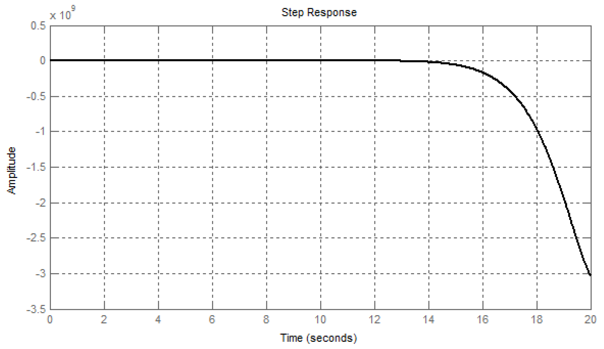
2.2. The Case When Even One Real Root Is Placed in the Right Half-Plane

If the frequency ω = 0, then the vector $\left(j^{\frac{1}{2}}\omega -p_1\right)$ occupies the position “−p₁”. If $\omega \to \infty$, then the rotation angle of the vector $\left(j^{\frac{1}{2}}\omega -p_1\right)$ is $\frac{3\pi }{4}$ by clockwise direction, i.e., the angle is negative. Then the total rotation angle of the vector, provided that the remaining roots are located in the left half-plane, can be calculated as follows:

$$\mathsf{\Delta }\phi = \left(n-1\right)\frac{\pi }{4}-\frac{3\pi }{4} = n \ast \frac{\pi }{4}-\pi$$

(14)

Here, $\mathsf{\Delta }\phi \ne n \ast \frac{\pi }{4}$, i.e., this value of ∆φ is due to the fact that the system is unstable (Figure 2).

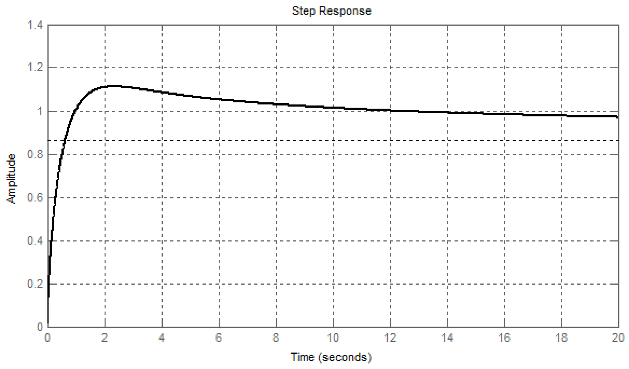
2.3. The Case When All Roots Are Complex-Conjugate Numbers with Negative Real Part

The resulting rotation angle of the vector $\left(j^{\frac{1}{2}}\omega -p_1\right)$ if the frequency changes from 0 to ∞ is equal to $\propto + \frac{\pi }{4}$ by counterclockwise direction, and the angle of rotation of the vector $\left(j^{\frac{1}{2}}\omega -p_2\right)$ is equal to $\propto -\frac{\pi }{4}$ clockwise, where $\propto$ is the angle due to complex roots. Thus, the total rotation angle of the vectors of a pair of complex-conjugate roots is equal to

$$\mathsf{\Delta }\phi = \frac{\pi }{4} + \propto -\left(\propto -\frac{\pi }{4}\right) = 2 \ast \frac{\pi }{4}$$

(15)

The rotation angle of the vector $H_n^{\ast }\left(j^{\frac{1}{2}}\omega \right)$, taking into account the rest of the similar roots, will be written as follows:

$$\mathsf{\Delta }\phi = \left(n-2\right)\frac{\pi }{4} + \frac{2\pi }{4} = n \ast \frac{\pi }{4}$$

(16)

Therefore, we conclude, that this value $\mathsf{\Delta }\phi$ is associated with a stable system–it is show on the Figure 3.

Example.

Given two poles of the fractional system in the basis j^1/2 on the left half-plane (p_1,2 = −0.5 ± j1.0), we obtain the following transfer function of the fractional system (Figure 4):

$$\mathrm{W}\left(s^{\frac{1}{2}}\right) = \frac{1}{{\left(s^{\frac{1}{2}}\right)}^2 + \left(s^{\frac{1}{2}}\right) + 1.25}$$

(17)

It is obvious that such a dynamic process corresponds to a stable system, and the stability condition is similar for integer order systems (the roots are in the left half-plane).

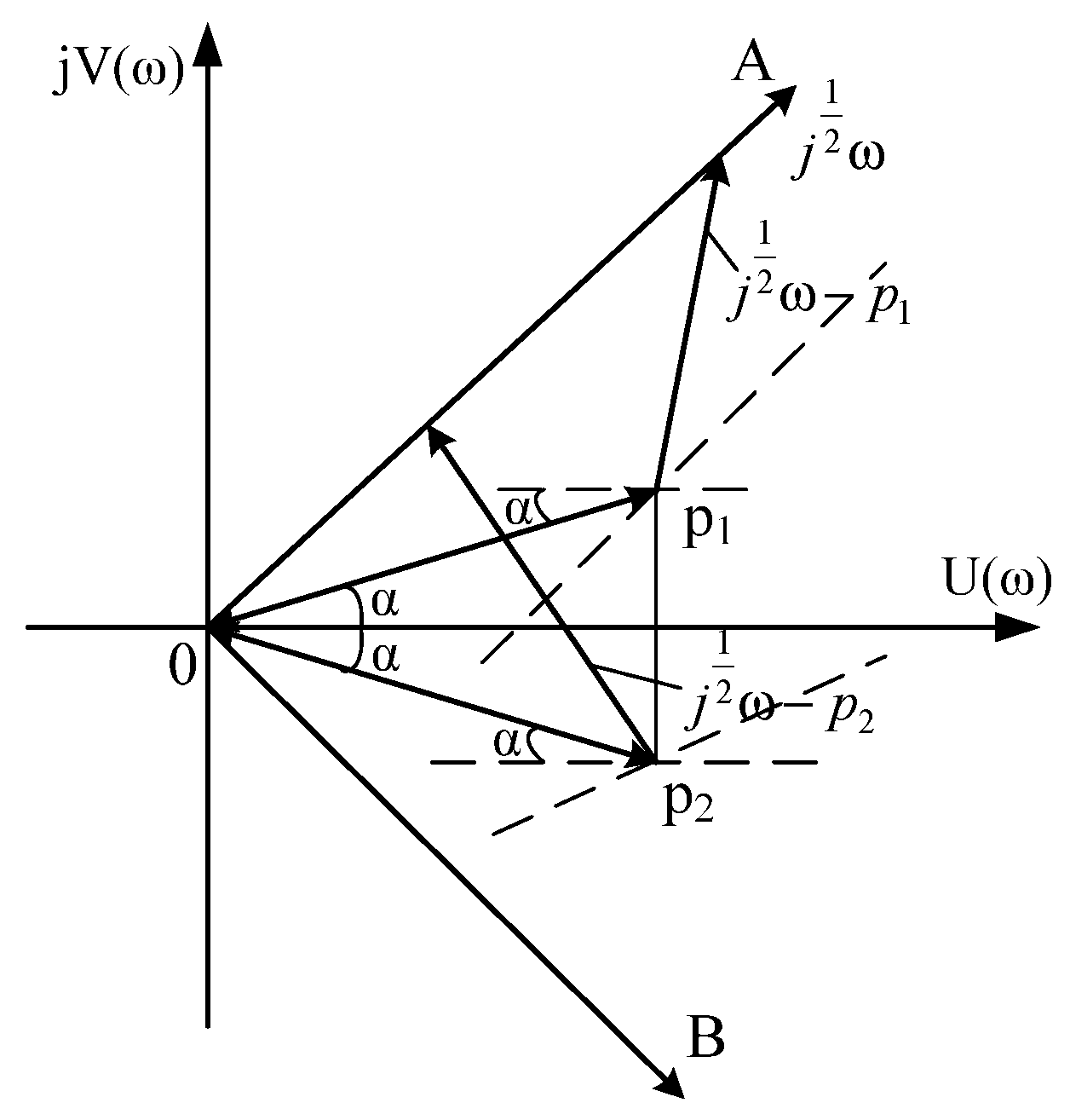
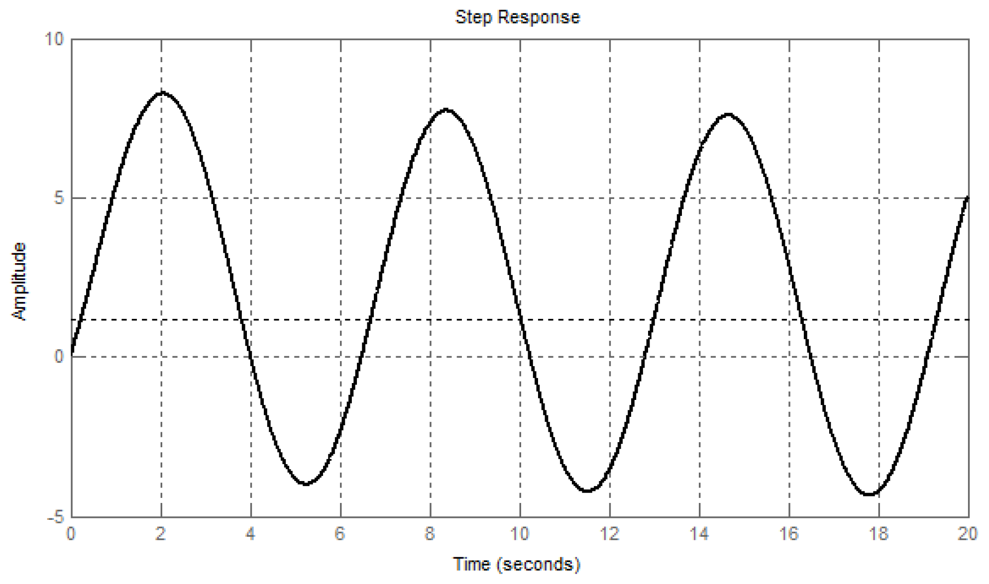
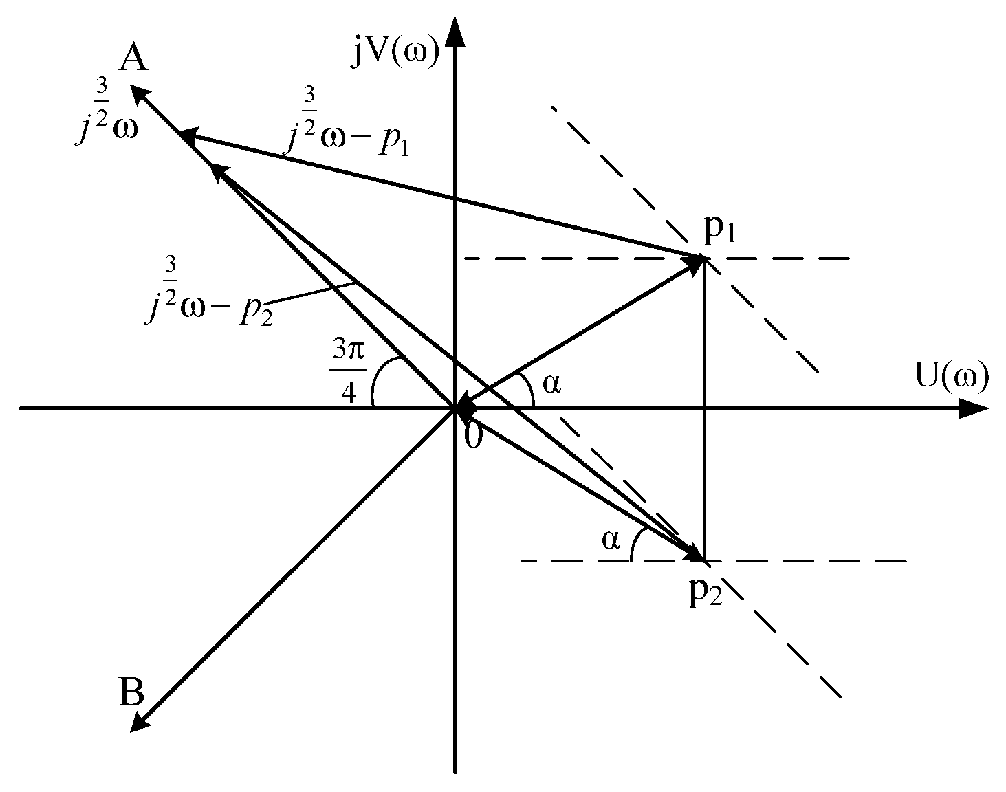
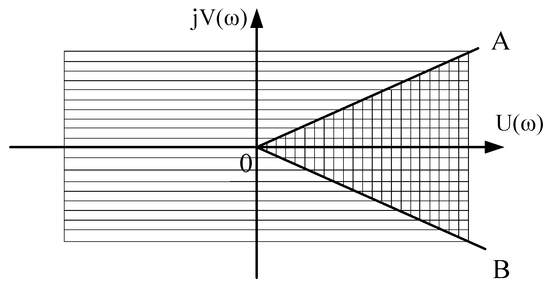
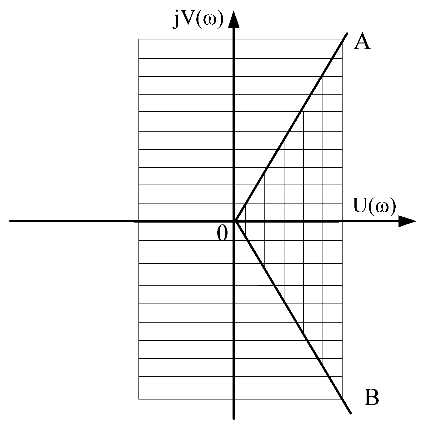
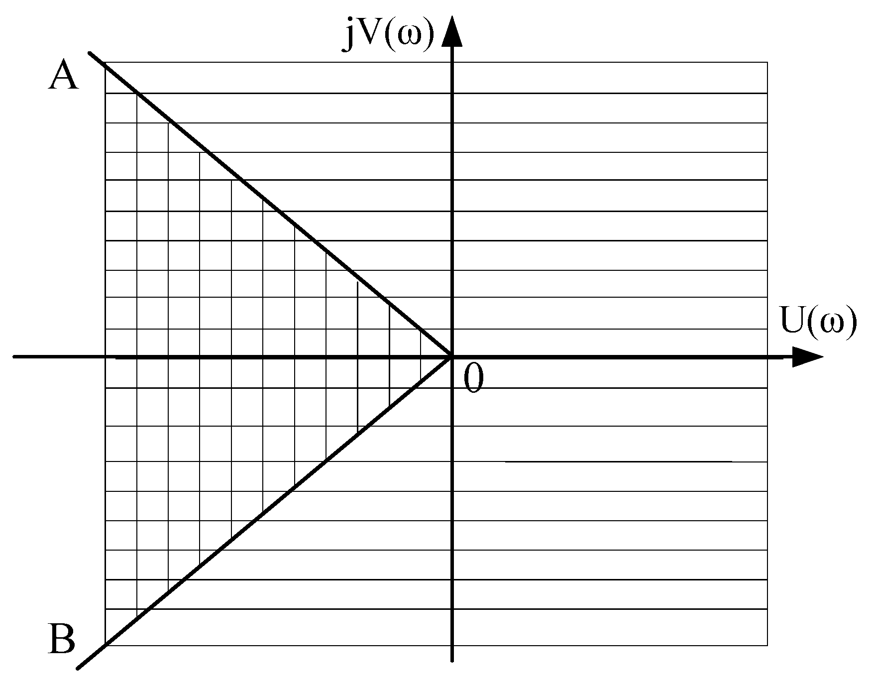
2.4. The Case When Even One Pair of Roots are Complex-Conjugate Numbers with a Positive Real Part (The Roots Are in the Sector AOB)

The area AOB is the area where the roots are when considering the polynomial basis $j^{\frac{l}{m}}$. In this case, the rotation angle of the vector $\left(j^{\frac{1}{2}}\omega -p_1\right)$ is equal $\left(\propto + \frac{\pi }{2} + \frac{\pi }{4}\right)$ by clockwise direction, if frequency changes from 0 to ∞ (the negative angle). The rotation angle of the vector $\left(j^{\frac{1}{2}}\omega -p_2\right)$, if $0\le \omega \le \infty ,$ is $\left(\frac{\pi }{2}-\propto + \frac{\pi }{4}\right),$ also a clockwise direction (negative angle). Therefore, the total rotation angle of the vectors for such pair of roots is as follows:

$$\mathsf{\Delta }\phi = -\propto -\frac{3\pi }{4}-\frac{3\pi }{4} + \propto = -2 \ast \frac{3\pi }{4}$$

(18)

Then, the resulting rotation angle of the vector $H_n^{\ast }\left(j^{\frac{1}{2}}\omega \right)$, taking into account that the remaining roots are stable, is equal to

$$\mathsf{\Delta }\phi = \left(n-2\right)\frac{\pi }{4}-2\frac{3\pi }{4}\ne n \ast \frac{\pi }{4}$$

(19)

Bearing in mind the obtained result, we will conclude that such system is not stable (Figure 5).

Example.

Given two poles of the fractional system in the basis j^1/2 into the sector AOB (p_1,2 = 1.0 ± j0.5), we obtain the following transfer function of the fractional system (Figure 6):

$$\mathrm{W}\left(s^{\frac{1}{2}}\right) = \frac{1}{{\left(s^{\frac{1}{2}}\right)}^2-2\left(s^{\frac{1}{2}}\right) + 1.25}$$

(20)

The obtained result indicates that this system is not stable. At the same way is indicated the value $\mathsf{\Delta }\mathsf{\phi }$, which was calculated for this case of the poles’ location on the complex plane.

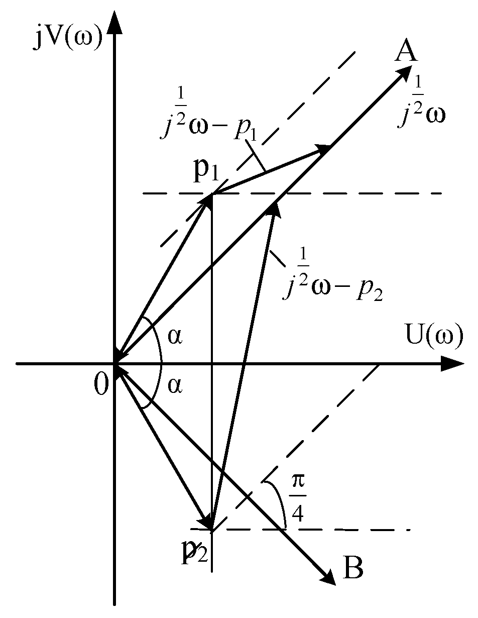
2.5. The Case of Complex-Conjugate Roots with a Positive Real Part (The Roots Are Outside the Sector AOB)

As reflected by Figure 7, the rotation angle of the vector $\left(j^{\frac{1}{2}}\omega -p_1\right)$ is equal to ($\frac{5\pi }{4}-\propto )$ (counterclockwise direction), and the rotation angle of the vector $\left(j^{\frac{1}{2}}\omega -p_2\right)$ is equal to $\left(\frac{3\pi }{4}-\propto \right)$ (clockwise direction).

Thus, in the case when the pair of complex-conjugate roots is outside of the sector AOB, the total rotation angle of the pair of roots will be equal to:

$$\mathsf{\Delta }\phi = \frac{5\pi }{4}-\propto -\left(\frac{3\pi }{4}-\propto \right) = 2 \ast \frac{\pi }{4}$$

(21)

Then, the total rotation angle of the vector $H_n^{\ast }\left(j^{\frac{1}{2}}\omega \right)$, taking into account the remaining roots, will be equal to:

$$\mathsf{\Delta }\phi = \left(n-2\right)\frac{\pi }{4} + 2\frac{2\pi }{4} = n \ast \frac{\pi }{4}$$

(22)

By analogy with the value of ∆φ for stable systems, we conclude that such a fractional order system is stable even with a positive real part of complex-conjugate roots.

Example.

Given two poles of the fractional system in the basis j^1/2, which are located outside the sector AOB (p_1,2 = 0.5 ± j1.0), the real part is positive. We obtain the following transfer function of the fractional system (Figure 8):

$$\mathrm{W}\left(s^{\frac{1}{2}}\right) = \frac{1}{{\left(s^{\frac{1}{2}}\right)}^2- \left(s^{\frac{1}{2}}\right) + 1.25}$$

(23)

The obtained result indicates that such a system is stable. The same way is indicated by the value $\mathsf{\Delta }\phi$, which is calculated for this location case of the poles on the complex plane. Now, shift to the case when the poles are located on the lines that form the sector AOB. It is hoped that such a system will be on the verge of stability. Let us check this in the following example.

Example.

Given two poles of the fractional system in the basis j^1/2 on the lines OA and OB (p_1,2 = 1.0 ± j1.0), we obtain the following transfer function of the fractional system (Figure 9):

$$\mathrm{W}\left(s^{\frac{1}{2}}\right) = \frac{1}{{\left(s^{\frac{1}{2}}\right)}^2-2\left(s^{\frac{1}{2}}\right) + 2}$$

(24)

The obtained result indicates that such a system is on the stability verge, i.e., the sector AOB divides the complex plane into stable and non-stable parts.

The last result does not fit into the classical condition of roots’ location in terms of system stability when we write the integer order transfer functions. It is obvious that, to describe the model of fractional systems, the non-stable condition of a system is transformed into the condition of finding the root in the corresponding sector of the right plane, but not in the full right half-plane. Therefore, checking the procedure is necessary to the rotation angles of the hodograph $H_n\left(j^{\frac{l}{m}}\omega \right)$ for different fractional orders of characteristic polynomials n when frequency changes in the range of $0\le \omega \le \infty .$ This will ensure the correctness of the hypothesis, if the total hodograph rotation angle of the vector $H_n\left(j^{\frac{l}{m}}\omega \right)$ based on the basis $\left(j^{\frac{l}{m}}\right)$ is equal to $n \ast \frac{\pi \ast l}{2 \ast m}$, where n is the characteristic polynomial order in the basis $\left(j^{\frac{l}{m}}\right)$. It should be noted that the order of a fractional characteristic polynomial can be as the highest frequency ω degree in the polynomial equation, which is written in either basis. Let us investigate hodographs for systems of different orders, which are represented by a characteristic polynomial in the basis j^1/2.

a. 

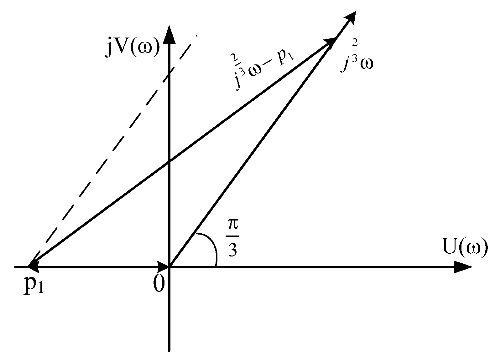
Hodograph of the second-order system

We write the characteristic polynomial in the basis j^1/2 as follows:

$$H_2\left(j^{\frac{1}{2}}\omega \right) = a_0{\left(j^{\frac{1}{2}}\omega \right)}^2 + a_1\left(j^{\frac{1}{2}}\omega \right) + a_2$$

(25)

Obviously, here n = 2. Let us write the representation of this expression in the basis j, using the equation $j^{\frac{1}{2}} = \frac{\sqrt{2}}{2}\left(1 + j\right)$. Then $U\left(\omega \right) = a_2 + a_1\frac{\sqrt{2}}{2}\omega$, the real part, and $V\left(\omega \right) = a_0{\omega }^2 + a_1\frac{\sqrt{2}}{2}\omega$, the imaginary part.

For ω = 0 we obtain $U\left(\omega \right) = a_2$ and $V\left(\omega \right) = 0$.

For ω = ∞ we obtain $U\left(\omega \right) = \infty$ and $V\left(\omega \right) = \infty$.

Therefore, $tg\left(\phi \right) = \frac{{\omega }^2\left(a_0 + \frac{a_1\sqrt{2}}{\omega 2}\right)}{{\omega }^2\left(\frac{a_2}{{\omega }_2} + \frac{a_1\sqrt{2}}{\omega 2}\right)}{|}_{\omega \to \infty } = \frac{a_0}{0} = \infty$.

Then $\phi = arctg\left(\infty \right) = \frac{\pi }{2} = 2\frac{\pi }{4}$.

The measure of the rotation angle of the vector $H_2\left(j^{\frac{1}{2}}\omega \right)$ obtained previously indicates that such a system is stable.

b. 

Hodograph of the third-order system

We write the characteristic polynomial in the basis j^1/2 for the case n = 3:

$$H_3\left(j^{\frac{1}{2}}\omega \right) = a_0{\left(j^{\frac{1}{2}}\omega \right)}^3 + a_1{\left(j^{\frac{1}{2}}\omega \right)}^2 + a_2\left(j^{\frac{1}{2}}\omega \right) + a_3$$

(26)

Rewrite the characteristic polynomial in the basis j. Using the formula j^1/2, write the equation as follows:

$$\begin{gathered} H_3\left(j^{\frac{1}{2}}\omega \right) = j{a}_0\frac{\sqrt{2}}{2}\left(1 + j\right){\omega }^3 + j{a}_1{\omega }^2 + a_2\frac{\sqrt{2}}{2}\left(1 + j\right)\omega + a_3 \\ = j{a}_0\frac{\sqrt{2}}{2}{\omega }^3-a_0\frac{\sqrt{2}}{2}{\omega }^3 + j{a}_1{\omega }^2 + a_2\frac{\sqrt{2}}{2}\omega + j{a}_2\frac{\sqrt{2}}{2}\omega + a_3 \end{gathered}$$

(27)

The expressions of the real and imaginary parts of this equation are written as:

$$\begin{gathered} U\left(\omega \right) = -a_0\frac{\sqrt{2}}{2}{\omega }^3 + a_2\frac{\sqrt{2}}{2}\omega + a_3, \\ V\left(\omega \right) = a_0\frac{\sqrt{2}}{2}{\omega }^3 + a_1{\omega }^2 + a_2\frac{\sqrt{2}}{2}\omega \end{gathered}$$

(28)

For ω = 0 obtain $U\left(\omega \right) = a_3 and V\left(\omega \right) = 0$.

If ω = ∞, the total rotation angle of the vector H₃(jω) can be represented as:

$$tg\left(\phi \right) = \frac{{\omega }^3\left(a_0\frac{\sqrt{2}}{2} + a_1\frac{1}{\omega } + \frac{a_2}{{\omega }^2}\frac{\sqrt{2}}{2}\right)}{{\omega }^3\left(-a_0\frac{\sqrt{2}}{2} + \frac{a_2}{{\omega }^2}\frac{\sqrt{2}}{2} + a_3\frac{1}{{\omega }^3}\right)}{|}_{\omega \to \infty } = \frac{a_0\frac{\sqrt{2}}{2}}{-a_0\frac{\sqrt{2}}{2}} = -1$$

(29)

Hence, $\mathsf{\Delta }\phi = arctg\left(-1\right)$. With provision for the signs V(ω) and U(ω) the angle is located in the second quadrant, i.e., $\mathsf{\Delta }\phi = \frac{3\pi }{4}$.

This value of the hodograph rotation angle corresponds to the stability condition. Let us check this condition with examples, in which we describe cases of three poles’ location in a different way on the complex plane. Suppose that one of the three poles is a real number and the other two and complex-conjugate numbers. Example:

(a). The real pole is in the left half-plane (p₁ = −1), and the two complex roots are located in the sector AOB (p_2,3 = 1.0 ± j0.5). In this case, the system is represented by the following transfer function (Figure 10):

$$\mathrm{W}\left(s^{\frac{1}{2}}\right) = \frac{1}{{\left(s^{\frac{1}{2}}\right)}^3-{\left(s^{\frac{1}{2}}\right)}^2-0.75\left(s^{\frac{1}{2}}\right) + 1.25}$$

(30)

From this, it follows that the real pole presence in the sector AOB indicates the unstable system mode.

(b). The real pole is in the left half-plane (p₁ = −1), and the two complex roots are located outside the AOB sector in the right half-plane (p_2,3 = 0.5 ± j1.0). In this case, the system is described by the following transfer function (Figure 11):

$$\mathrm{W}\left(s^{\frac{1}{2}}\right) = \frac{1}{{\left(s^{\frac{1}{2}}\right)}^3 + 0.25\left(s^{\frac{1}{2}}\right) + 1.25}$$

(31)

The obtained transient function indicates that for the third-order system, the poles’ location is outside of the sector AOB and corresponds to a stable system.

(c). The real pole is in the right half-plane (p₁ = 1), and the two complex roots are located outside of the sector AOB in the right half-plane, too (p_2,3 = 0.5 ± j1.0). In this case, the system is represented by the following transfer function:

$$\mathrm{W}\left(s^{\frac{1}{2}}\right) = \frac{1}{{\left(s^{\frac{1}{2}}\right)}^3-2{\left(s^{\frac{1}{2}}\right)}^2 + 2.25\left(s^{\frac{1}{2}}\right) - 1.25}$$

(32)

Figure 12 shows that such a fractional system is not stable. Therefore, the presence of one or more poles in the sector AOB indicates the system instability.

c. 

Fifth-order hodograph

Let us write the characteristic polynomial in the basis j^1/2 for the case n = 5:

$$H_5\left(j^{\frac{1}{2}}\omega \right) = a_0{\left(j^{\frac{1}{2}}\omega \right)}^5 + a_1{\left(j^{\frac{1}{2}}\omega \right)}^4 + a_2{\left(j^{\frac{1}{2}}\omega \right)}^3 + a_3{\left(j^{\frac{1}{2}}\omega \right)}^2 + a_4{\left(j^{\frac{1}{2}}\omega \right)}^1 + a_5$$

(33)

Given that:

$$j^{\frac{5}{2}} = -\frac{\sqrt{2}}{2}\left(1 + j\right); j^{\frac{4}{2}} = -1; j^{\frac{3}{2}} = j\frac{\sqrt{2}}{2}\left(1 + j\right); j^{\frac{1}{2}} = \frac{\sqrt{2}}{2}\left(1 + j\right)$$

(34)

the characteristic polynomial $H_5\left(j^{\frac{1}{2}}\omega \right)$ in basis j will take the form:

$$\begin{gathered} H_5\left(j\omega \right) = -a_0\frac{\sqrt{2}}{2}\left(1 + j\right){\omega }^5-a_1{\omega }^4 + a_2\frac{\sqrt{2}}{2}\left(-1 + j\right){\omega }^3 + a_{3}j{\omega }^2 \\ + a_4\frac{\sqrt{2}}{2}\left(1 + j\right)\omega + a_5 \end{gathered}$$

(35)

Extracting the real and imaginary part, we get

$$\begin{gathered} U\left(\omega \right) = -a_0\frac{\sqrt{2}}{2}{\omega }^5-a_1{\omega }^4-a_2\frac{\sqrt{2}}{2}{\omega }^3 + a_4\frac{\sqrt{2}}{2}\omega + a_5, \\ V\left(\omega \right) = -a_0\frac{\sqrt{2}}{2}{\omega }^5 + a_2\frac{\sqrt{2}}{2}{\omega }^3 + a_3{\omega }^2 + a_4\frac{\sqrt{2}}{2}\omega \end{gathered}$$

(36)

According to these expressions, we analyze the hodograph in the basis j. If ω = 0, then U(ω) = a₅ and V(ω) = 0. If ω = ∞, write the expression for tgφ in the form:

$$tg\left(\phi \right) = \frac{{\omega }^5\left(-a_0\frac{\sqrt{2}}{2} + \frac{a_2}{{\omega }^2}\frac{\sqrt{2}}{2} + a_3\frac{1}{{\omega }^3} + \frac{a_4}{{\omega }^4}\frac{\sqrt{2}}{2}\right)}{{\omega }^5\left(-a_0\frac{\sqrt{2}}{2}-a_1\frac{1}{\omega }-\frac{a_2}{{\omega }^2}\frac{\sqrt{2}}{2} + \frac{a_4}{{\omega }^4}\frac{\sqrt{2}}{2} + a_5\frac{1}{{\omega }^5}\right)}{|}_{\omega \to \infty } = \frac{-a_0\frac{\sqrt{2}}{2}}{-a_0\frac{\sqrt{2}}{2}} = 1$$

(37)

We get $\mathsf{\Delta }\phi = arctg\left(\frac{-1}{-1}\right) = 5\frac{\pi }{4}$.

Therefore, the hodograph of the vector $H_5\left(j^{\frac{1}{2}}\omega \right)$ turns to the angle $5\frac{\pi }{4}$ in the basis j when the frequency changes from 0 to ∞, and this corresponds to the stability condition, which is shown above. Next, we take as a basis j^1/3 for the characteristic polynomial creation.

Given the Moivre formula for the case l = 1 and m = 3, rewrite the equation

$$\sqrt[3]{j} = \sqrt[3]{1}\left(cos\frac{\frac{\pi }{2} + 2k\pi }{m} + jsin\frac{\frac{\pi }{2} + 2k\pi }{m}\right)$$

(38)

When k = 0, we obtain

$$\sqrt[3]{j} = cos\frac{\pi }{2 \ast 3} + jsin\frac{\pi }{2 \ast 3} = \frac{\sqrt{3}}{2} + j\frac{1}{2} = \frac{1}{2}\left(\sqrt{3} + j\right)$$

(39)

Now formulate a polynomial in the basis j^1/3, as the following equation

$$H_n\left(j^{\frac{1}{3}}\omega \right) = a_0{\left(j^{\frac{1}{3}}\omega \right)}^n + a_1{\left(j^{\frac{1}{3}}\omega \right)}^{n-1} + a_2{\left(j^{\frac{1}{3}}\omega \right)}^{n-2} + \dots + a_{n-1}\left(j^{\frac{1}{3}}\omega \right) + a_n$$

(40)

and write it as

$$H_n^{\ast }\left(j^{\frac{1}{3}}\omega \right) = a_0\left(j^{\frac{1}{3}}\omega -p_1\right) \ast \left(j^{\frac{1}{3}}\omega -p_2\right) \dots \left(j^{\frac{1}{3}}\omega -p_{n-1}\right) \ast \left(j^{\frac{1}{3}}\omega -p_n\right)$$

(41)

Let us analyze variations of the root location on the complex plane jV(ω), U(ω), and the value of total rotation angles of the vectors $\left(j^{\frac{1}{3}}\omega -p_1\right)$ when the frequency changes from 0 to infinity. Note that, according to this criterion, the total rotation angle of the vector $H_n^{\ast }\left(j^{\frac{1}{3}}\omega \right)$ when the frequency changes from 0 to infinity must be equal to $\mathsf{\Delta }\phi = n\frac{\pi l}{2m}$ where n is the polynomial order.

3. Analysis of the Influence of Roots’ Location of a Characteristic Polynomial ${\mathit{H}}_{\mathit{n}}^{\mathbf{*}}\left({\mathit{j}}^{\frac{\mathbf{1}}{\mathbf{3}}}\mathit{\omega }\right)$ on the System Stability

The trigonometric formula for j^1/3 is given as

$$j^{\frac{1}{3}} = l\left(cos\frac{\frac{\pi }{2} + 2k\pi }{3} + jsin\frac{\frac{\pi }{2} + 2k\pi }{3}\right)$$

(42)

For k = 0 we get

$$j^{\frac{1}{3}} = l\left(cos\frac{\pi }{6} + jsin\frac{\pi }{6}\right) = \frac{1}{2}(\sqrt{3} + j)$$

(43)

3.1. All Roots Are Real Numbers and Are Located on the Left Half-Plane

For frequency ω = 0 and the vector $\left(j^{\frac{1}{3}}\omega -p_1\right),$ state the position +p₁. As the frequency increases to ω = ∞, the rotation angle of the vector $\left(j^{\frac{1}{3}}\omega -p_1\right)$ will be equal $+ \frac{\pi }{6}$ (by counterclockwise direction) [28,29,30]. Therefore, the total rotation angle of the vector $H_n^{\ast }\left(j^{\frac{1}{3}}\omega \right),$ when taking into account all roots n, is given as:

$$\mathsf{\Delta }\phi = \left(n-1\right)\frac{\pi }{6} + \frac{\pi }{6} = n \ast \frac{\pi }{6}$$

(44)

Thus, in this case for a stable system, the resulting angle of rotation of the vector $H_n^{\ast }\left(j^{\frac{1}{3}}\omega \right)$ when the frequency changes from zero to infinity takes the value $n\frac{\pi }{6}$, by analogy with the Mikhailov’s criterion and in according to criterion [7]—see Figure 13.

3.2. The Case When Even One Real Root Is Placed in the Right Half-Plane

If the frequency ω = 0, then the vector $\left(j^{\frac{1}{3}}\omega -p_1\right)$ sets the position −p₁. If ω = 0, then the rotation angle of the vector $\left(j^{\frac{1}{3}}\omega -p_1\right)$ is by clockwise direction, i.e., the angle is negative. Then the total rotation angle of the vector, provided that the remaining roots are located in the left half-plane, can be calculated as follows (Figure 14):

$$\mathsf{\Delta }\phi = \left(n-1\right)\frac{\pi }{6}-5\frac{\pi }{6} = n \ast \frac{\pi }{6}-\pi$$

(45)

Here, $\mathsf{\Delta }\phi \ne n\frac{\pi }{6}$, i.e., this value of ∆φ is due to the fact that the system is unstable.

3.3. The Case When All Roots Are Complex-Conjugate Numbers with a Negative Real Part

The total rotation angle of the vector $\left(j^{\frac{1}{3}}\omega -p_1\right)$ when the frequency changes from 0 to ∞ is equal to $\frac{\pi }{6} + \propto$ by counterclockwise direction, and the rotation angle of the vector $\left(j^{\frac{1}{3}}\omega -p_2\right)$ is equal to $\propto -\frac{\pi }{6}$ by clockwise direction. Thus, the total rotation angle of the vectors of a pair of complex-conjugate roots is equal to:

$$\mathsf{\Delta }\phi = \frac{\pi }{6} + \propto - \left(\propto -\frac{\pi }{6}\right) = 2\frac{\pi }{6}$$

(46)

The rotation angle of the vector $H_n^{\ast }\left(j^{\frac{1}{3}}\omega \right),$ taking into account the other similar roots, will be written as follows:

$$\mathsf{\Delta }\phi = \left(n-2\right)\frac{\pi }{6} + \frac{2\pi }{6} = n \ast \frac{\pi }{6}$$

(47)

Therefore, we conclude that this value ∆φ is associated with a stable system (Figure 15).

3.4. The Case When Even One Pair of Roots is Complex-Conjugate Numbers with a Positive Real Part (The Roots Are in the Middle of the Sector AOB)

In this case, the rotation angle of the vector $\left(j^{\frac{1}{3}}\omega -p_1\right),$ when ω changes from zero to ∞, equals $\propto + 5\frac{\pi }{6}$ (by clockwise direction (the negative angle)). The rotation angle of the vector $\left(j^{\frac{1}{3}}\omega -p_2\right),$ if 0 ≤ ω ≤ ∞, equals $5\frac{\pi }{6}-\propto$ also by clockwise direction (negative angle). Therefore, the total rotation angle of the vectors for such a pair of roots is as follows:

$$\mathsf{\Delta }\phi = -\propto -\frac{5\pi }{6}-\frac{5\pi }{6} + \propto = -2\frac{5\pi }{6}$$

(48)

Then the total rotation angle of the vector $H_n^{\ast }\left(j^{\frac{1}{3}}\omega \right),$ taking into account that the other remaining roots are stable, is given by equation (Figure 16):

$$\mathsf{\Delta }\phi = \left(n-2\right)\frac{\pi }{6}- \left(\frac{5\pi }{6} + \propto \right) - \left(\frac{5\pi }{6}-\propto \right) = n\frac{\pi }{6}-12\frac{\pi }{6}<n\frac{\pi }{6}$$

(49)

With the obtained result, we conclude that such a system is not stable.

3.5. The Case of Complex-Conjugate Roots with a Positive Real Part (The Roots Are Outside the Sector AOB)

As we can see in Figure 17, the rotation angle of the vector $\left(j^{\frac{1}{3}}\omega -p_1\right)$ is equal to $\left(\frac{7\pi }{6}-\propto \right)$ (by counterclockwise direction), and the rotation angle of the vector $\left(j^{\frac{1}{3}}\omega -p_1\right)$ is equal to $-\left(\frac{5\pi }{6}-\propto \right)$ (by clockwise direction).

Thus, in the case when the pair of complex-conjugate roots is outside the sector AOB, the total rotation angle of the pair of roots is given by equation

$$\mathsf{\Delta }\phi = \frac{7\pi }{6}-\propto - \left(\frac{5\pi }{6}-\propto \right) = 2\frac{\pi }{6}$$

(50)

Then, the total rotation angle of the vector $H_n^{\ast }\left(j^{\frac{1}{3}}\omega \right),$ taking into account the remaining roots, will be equal to

$$\mathsf{\Delta }\phi = \left(n-2\right)\frac{\pi }{6} + \frac{2\pi }{6} = n\frac{\pi }{6}$$

(51)

By analogy with the value of ∆φ for stable systems, we conclude that such a fractional order system is stable even with a positive real part of complex-conjugate roots. Here, we also investigate hodographs of vectors $H_n^{\ast }\left(j^{\frac{1}{3}}\omega \right)$ for systems of different orders, which are represented by a characteristic polynomial in the basis j^1/3.

a. 

Hodograph of the second-order system

The characteristic polynomial in the basis j^1/3 is given by equation:

$$H_2\left(j^{\frac{1}{3}}\omega \right) = a_0{\left(j^{\frac{1}{3}}\omega \right)}^2 + a_1\left(j^{\frac{1}{3}}\omega \right) + a_2$$

(52)

Let us represent this expression in the basis j, using formulas

$$j^{\frac{1}{3}} = \frac{1}{2}\left(\sqrt{3} + j\right), j^{\frac{2}{3}} = \frac{1}{2}\left(1 + j\sqrt{3}\right)$$

(53)

Therefore,

$$H_2\left(j\omega \right) = a_0\frac{1}{2}\left(1 + j\sqrt{3}\right){\omega }^2 + a_1\frac{1}{2}\left(\sqrt{3} + j\right)\omega + a_2$$

(54)

Then,

$$U\left(\omega \right) = \frac{1}{2}{a}_0{\omega }^2 + \frac{1}{2}{a}_1\omega \sqrt{3} + a_2, \mathrm{the} \mathrm{real} \mathrm{part}, \mathrm{and}$$

(55)

$$V\left(\omega \right) = \frac{1}{2}{a}_0\sqrt{3}{\omega }^2 + \frac{1}{2}{a}_1\omega , \mathrm{the} \mathrm{imaginary} \mathrm{part}.$$

(56)

For ω = 0 we obtain U(ω) = a₂ and V(ω) = 0.

For ω = ∞ we obtain U(ω) = ∞ and V(ω) = ∞.

$$tg\left(\phi \right) = \frac{{\omega }^2\left(\frac{1}{2}{a}_0\sqrt{3} + \frac{1}{2}{a}_1\frac{1}{\omega }\right)}{{\omega }^2\left(\frac{1}{2}{a}_0 + \frac{1}{2}{a}_1\sqrt{3}\frac{1}{\omega } + a_2\frac{1}{{\omega }^2}\right)}{|}_{\omega \to \infty } = \sqrt{3}$$

(57)

Then, $\phi = arctg\sqrt{3} = {60}^0 = 2\frac{\pi }{6}$. The measure of the rotation angle of the vector $H_2\left(j^{\frac{1}{3}}\omega \right)$ obtained above indicates that such a system is stable. Therefore, it all adds up to that the analysis of the fractional system stability can be developed on the hodograph of the characteristic polynomial in the basis j, which corresponds to the characteristic polynomial in the basis j^1/3.

Example.

(a) Given two poles of the fractional system in the basis j^1/3 in the sector AOB (p_1,2 = 1.0 ± j0.1), we obtain the following transfer function of the fractional system (Figure 18):

$$\mathrm{W}\left(s^{\frac{1}{3}}\right) = \frac{1}{{\left(s^{\frac{1}{3}}\right)}^2-2\left(s^{\frac{1}{3}}\right) + 1.01}$$

(58)

The obtained result indicates that such a system is not stable. The value ∆φ calculated for this case by the poles’ location on the complex plane points to the same.

(b) Given two poles of the fractional system in the basis j^1/3 outside the sector AOB (p_1,2 = 0.5 ± j1) in the right half-plane, we obtain the following transfer function of the fractional system (Figure 19):

$$\mathrm{W}\left(s^{\frac{1}{3}}\right) = \frac{1}{{\left(s^{\frac{1}{3}}\right)}^2- \left(s^{\frac{1}{3}}\right) + 1.25}$$

(59)

The obtained result points to the stability of such a system. The value ∆φ indicates the same.

(c) Given two poles of the fractional system in the basis j^1/3 on the lines OA and OB (p_1,2 = 0.5$\sqrt{3}$ ± j0.5), we obtain the following transfer function of the fractional system (Figure 20):

$$\mathrm{W}\left(s^{\frac{1}{3}}\right) = \frac{1}{{\left(s^{\frac{1}{3}}\right)}^2- \sqrt{3}\left(s^{\frac{1}{3}}\right) + 1}$$

(60)

The obtained result indicates that such a system is on critical stability, i.e., the sector AOB divides the complex plane into stable and non-stable parts, similarly to the case for the basis j^1/2.

b. 

Hodograph of the third-order system

The characteristic polynomial in the basis j^1/3 for the case n = 3:

$$H_3\left(j^{\frac{1}{3}}\omega \right) = a_0{\left(j^{\frac{1}{3}}\omega \right)}^3 + a_1{\left(j^{\frac{1}{3}}\omega \right)}^2 + a_2\left(j^{\frac{1}{3}}\omega \right) + a_3$$

(61)

Let us represent the characteristic polynomial in the basis j. Using the formula j^1/3, we give:

$$H_3\left(j\omega \right) = a_{0}j{\omega }^3 + a_1\frac{1}{2}\left(1 + j\sqrt{3}\right){\omega }^2 + a_2\frac{1}{2}\left(\sqrt{3} + j\right)\omega + a_3$$

(62)

Then the equations of the real and imaginary parts are follows:

$$U\left(\omega \right) = a_1{\omega }^2 + \frac{1}{2}{a}_2\omega \sqrt{3} + a_3,$$

(63)

$$V\left(\omega \right) = a_0{\omega }^3 + \frac{1}{2}{a}_1\sqrt{3}{\omega }^2 + a_2\frac{1}{2}\omega$$

(64)

For ω = 0 we obtain U(ω) = a₃ and V(ω) = 0.

If ω = ∞, the total rotation angle of the vector H₃(jω) is given by the equation:

$$tg\left(\phi \right) = \frac{{\omega }^3\left(a_0 + \frac{1}{2}{a}_1\sqrt{3}\frac{1}{\omega } + \frac{1}{2}{a}_2\frac{1}{{\omega }^2}\right)}{{\omega }^3\left(\frac{1}{2}{a}_1\frac{1}{\omega } + \frac{1}{2}{a}_2\sqrt{3}\frac{1}{{\omega }^2} + a_3\frac{1}{{\omega }^3}\right)}{|}_{\omega \to \infty } = \infty$$

(65)

Hence, $\mathsf{\Delta }\phi = arctg\infty = \frac{\pi }{2} = 3\frac{\pi }{6}$. Given the signs V(ω) and U(ω), the angle is located in the first quadrant, i.e., $\mathsf{\Delta }\phi = 3\frac{\pi }{6}$. This value of the rotation angle of the hodograph corresponds to the stability condition.

c. 

Fifth-order hodograph

The characteristic polynomial in the basis j^1/3 for the case n = 5 is given as:

$$H_5\left(j^{\frac{1}{3}}\omega \right) = a_0{\left(j^{\frac{1}{3}}\omega \right)}^5 + a_1{\left(j^{\frac{1}{3}}\omega \right)}^4 + a_2{\left(j^{\frac{1}{3}}\omega \right)}^3 + a_3{\left(j^{\frac{1}{3}}\omega \right)}^2 + a_4\left(j^{\frac{1}{3}}\omega \right) + a_5$$

(66)

Let us turn to the characteristic polynomial in the basis j. Given that

$$j^{\frac{1}{3}} = \frac{1}{2}\left(\sqrt{3} + j\right), j^{\frac{2}{3}} = \frac{1}{2}\left(1 + j\sqrt{3}\right)$$

(67)

$$j^{\frac{4}{3}} = j\frac{1}{2}\left(\sqrt{3} + j\right) = \frac{1}{2}\left(j\sqrt{3}-1\right), j^{\frac{5}{3}} = j \ast j^{\frac{2}{3}} = j\frac{1}{2}-\frac{\sqrt{3}}{2} = \frac{1}{2}(j-\sqrt{3})$$

(68)

The characteristic polynomial$H_5\left(j^{\frac{1}{3}}\omega \right)$ in basis j is given by the equation:

$$\begin{gathered} H_5\left(j\omega \right) = a_0\frac{1}{2}\left(j-\sqrt{3}\right){\omega }^5 + a_1\frac{1}{2}\left(j\sqrt{3}-1\right){\omega }^4 + a_{2}j{\omega }^3 + a_3\frac{1}{2}\left(1 + j\sqrt{3}\right){\omega }^2 \\ + a_4\frac{1}{2}\left(\sqrt{3} + j\right)\omega + a_5 \end{gathered}$$

(69)

Extract the real and imaginary parts and write the following equations

$$U\left(\omega \right) = -a_0\frac{1}{2}\sqrt{3}{\omega }^5-a_1\frac{1}{2}{\omega }^4 + a_3\frac{1}{2}{\omega }^2 + \frac{1}{2}\sqrt{3}{a}_4\omega + a_5,$$

(70)

$$V\left(\omega \right) = a_0\frac{1}{2}{\omega }^5 + \frac{1}{2}{a}_1\sqrt{3}{\omega }^4 + a_2{\omega }^3 + a_3\frac{1}{2}\sqrt{3}{\omega }^2 + a_4\frac{1}{2}\omega$$

(71)

According to these equations, we analyze the hodograph in the basis j. If ω = 0, then U(ω) = a₅ and V(ω) = 0. If ω = ∞, then write the equation for tgφ as

$$\begin{gathered} tg\left(\phi \right) = \frac{{\omega }^5\left(a_0\frac{1}{2} + \frac{1}{2}{a}_1\sqrt{3}\frac{1}{\omega } + a_2\frac{1}{{\omega }^2} + \frac{1}{2}{a}_3\sqrt{3}\frac{1}{{\omega }^3} + a_4\frac{1}{2}\frac{1}{{\omega }^4}\right)}{-{\omega }^5\left(a_0\frac{1}{2}\sqrt{3} + \frac{1}{2}{a}_1\frac{1}{\omega }-\frac{1}{2}{a}_3\frac{1}{{\omega }^3}-\frac{1}{2}{a}_4\sqrt{3}\frac{1}{{\omega }^4}-a_5\frac{1}{{\omega }^5}\right)}{|}_{\omega \to \infty } \\ = \frac{a_0\frac{1}{2}}{-a_0\frac{1}{2}\sqrt{3}} = -\frac{1}{\sqrt{3}} \end{gathered}$$

(72)

We will give $\mathsf{\Delta }\phi = arctg\left(-\frac{1}{\sqrt{3}}\right) = 5\frac{\pi }{6}$.

Therefore, when the frequency changes from 0 to ∞, the hodograph of the vector $H_5\left(j^{\frac{1}{3}}\omega \right)$ in the basis j turns to the angle $\frac{5\pi }{6}$, and this corresponds to the stability condition, which is described above.

Thus, the obtained values of vectors $H_n\left(j^{\frac{1}{3}}\omega \right)$ hodographs when ω = 0 and ω = ∞ agree to the conditions of the above criterion of the fractional system stability.

Next, we take as a basis the characteristic polynomial –j^2/3.

4. Analysis of the Influence of the Characteristic Polynomial Roots’ Location ${\displaystyle {\mathit{H}}_{\mathit{n}}^{\mathbf{*}}\left({\mathit{j}}^{\frac{\mathbf{2}}{\mathbf{3}}}\mathit{\omega }\right)}$ on System Stability

Trigonometric representation for j^2/3 is written as

$$j^{\frac{2}{3}} = 1\left(cos\frac{2\left(\frac{\pi }{2} + 2k\pi \right)}{3} + jsin\frac{2\left(\frac{\pi }{2} + 2k\pi \right)}{3}\right)$$

(73)

For k = 0, we obtain

$$j^{\frac{2}{3}} = 1\left(cos\frac{\pi }{3} + jsin\frac{\pi }{3}\right) = \frac{1}{2} + j\frac{\sqrt{3}}{2} = \frac{1}{2}(1 + j\sqrt{3})$$

(74)

Now, write the equation for $H_n\left(j^{\frac{2}{3}}\omega \right)$ as

$$H_n^{\ast }\left(j^{\frac{2}{3}}\omega \right) = a_0\left(j^{\frac{2}{3}}\omega -p_1\right) \ast \left(j^{\frac{2}{3}}\omega -p_2\right) \dots \left(j^{\frac{2}{3}}\omega -p_{n-1}\right) \ast \left(j^{\frac{2}{3}}\omega -p_n\right)$$

(75)

and perform the above analysis.

4.1. All Roots Are Real Numbers and Are Located on the Left Half-Plane

For the frequency ω = 0, vector $\left(j^{\frac{2}{3}}\omega -p_1\right)$ takes the position +p₁ (Figure 21). With increasing frequency up to ω = 0, the rotation angle of vector $\left(j^{\frac{2}{3}}\omega -p_1\right)$ will be equal to $\frac{\pi }{3}$ (counterclockwise rotation direction) [31,32,33]. Thus, the total rotation angle of vector $H_n^{\ast }\left(j^{\frac{2}{3}}\omega \right)$, with taking into account n number of roots, is written by the equation:

$$\mathsf{\Delta }\phi = \left(n-1\right)\frac{\pi }{3} + l\frac{\pi }{3} = n\frac{\pi }{3}$$

(76)

Thus, by analogy with the Mikhailov’s criterion and in accordance with the criterion [7], in this case, for a stable system, the resulting rotation angle of the vector $H_n^{\ast }\left(j^{\frac{2}{3}}\omega \right)$ when the frequency changes from zero to infinity takes the value $n\frac{\pi }{3}$.

4.2. The Case When Even One Real Root Is Located in the Right Half-Plane

If ω = 0, then vector $\left(j^{\frac{2}{3}}\omega -p_1\right)$ takes a place –p₁. If $\omega \to \infty$, then the rotation angle of the vector $\left(j^{\frac{2}{3}}\omega -p_1\right)$ equals $2\frac{\pi }{3}$ (clockwise direction), that is, the negative angle. Then the total rotation angle of the vector, provided that the remaining roots are located in the left half-plane, can be calculated as follows:

$$\mathsf{\Delta }\phi = \left(n-1\right)\frac{\pi }{3}-2\frac{\pi }{3} = n\frac{\pi }{3}-\pi$$

(77)

In this $\mathsf{\Delta }\phi \ne n\frac{\pi }{3}$, that is, such a value of ∆φ is due to the fact that the system is unstable (Figure 22).

4.3. The Case When All Roots Are Complex-Conjugate Numbers with a Negative Real Part

The total rotation angle of the vector $\left(j^{\frac{2}{3}}\omega -p_1\right),$ provided the frequency changes from 0 to ∞, is equal to $\left(\propto + \frac{\pi }{3}\right)$ by counterclockwise direction, and the rotation angle of the vector $\left(j^{\frac{2}{3}}\omega -p_2\right)$ is equal to $\left(\propto -\frac{\pi }{3}\right)$ by clockwise direction (Figure 23). Thus, the resulting rotation angle of the vectors of a pair of complex-conjugate roots is equal to

$$\mathsf{\Delta }\phi = \propto + \frac{\pi }{3}- \left(\propto -\frac{\pi }{3}\right) = 2\frac{\pi }{3}$$

(78)

The rotation angle of the vectors $H_n^{\ast }\left(j^{\frac{2}{3}}\omega \right),$ taking into account the rest of the similar roots, is written as the following equation:

$$\mathsf{\Delta }\phi = \left(n-2\right)\frac{\pi }{3} + \frac{\pi }{3} + \propto -\propto + \frac{\pi }{3} = n\frac{\pi }{3}$$

(79)

Therefore, we conclude that this value is associated with a stable system.

4.4. The Case When Even One Pair of Roots is Complex-Conjugate Numbers with a Positive Real Part (The Roots Are in the Sector AOB)

For this case, the rotation angle of the vector $\left(j^{\frac{2}{3}}\omega -p_1\right),$ when ω changes from zero to ∞, is equal to $\left(\propto + 2\frac{\pi }{3}\right)$ by clockwise direction (negative angle). The rotation angle of the vector $\left(j^{\frac{2}{3}}\omega -p_2\right),$ if $0\le \omega \le \infty$, is equal to $\left(2\frac{\pi }{3}-\propto \right)$ by clockwise direction too. Therefore, the total rotation angle of the vectors for such a pair of roots is as follows:

$$\mathsf{\Delta }\phi = -\propto + \frac{2\pi }{3}-\frac{2\pi }{3} + \propto = -4\frac{\pi }{3}$$

(80)

Then, the total rotation angle of the vector $H_n^{\ast }\left(j^{\frac{2}{3}}\omega \right),$ given that the remaining roots are stable and equal, is (Figure 24):

$$\mathsf{\Delta }\phi = \left(n-2\right)\frac{\pi }{3}-4\frac{\pi }{3} = n\frac{\pi }{3}-6\frac{\pi }{3}<n\frac{\pi }{3}$$

(81)

Taking into account the obtained result, we can conclude that such a system is unstable.

4.5. The Case of Complex-Conjugate Roots with a Positive Real Part (The Roots Are Outside the AOB Sector)

As is clear from figure of the vector $\left(j^{\frac{2}{3}}\omega -p_1\right), \mathrm{the}$ rotation angle is equal to $\left(4\frac{\pi }{3}-\propto \right)$ in the positive direction, and rotation angle of the vector $\left(j^{\frac{2}{3}}\omega -p_2\right)$ is equal to $-\left(-\propto + 2\frac{\pi }{3}\right)$ in the negative direction (Figure 25).

Thus, in the case when the pair of complex-conjugate roots is outside the sector AOB, the resulting rotation angle of the pair of roots will be equal to:

$$\mathsf{\Delta }\phi = \frac{4\pi }{3}-\propto - \left(\frac{2\pi }{3}-\propto \right) = 2\frac{\pi }{3}$$

(82)

Then, the total rotation angle of the vector $H_n^{\ast }\left(j^{\frac{2}{3}}\omega \right),$ when taking into account other roots, is described as:

$$\mathsf{\Delta }\phi = \left(n-2\right)\frac{\pi }{3}-\propto + \frac{4\pi }{3} + \propto - \frac{2\pi }{3} = n\frac{\pi }{3}$$

(83)

By analogy with the value ∆φ for stable system, we conclude that such a fractional order system is stable even with a positive real part of complex-conjugate roots. Let us investigate hodographs for systems of different orders, which are represented by a characteristic polynomial in the basis j^2/3.

a. 

Hodograph of the second-order system

We write the characteristic polynomial in the basis j^2/3 by the way of:

$$H_2\left(j^{\frac{2}{3}}\omega \right) = a_0{\left(j^{\frac{2}{3}}\omega \right)}^2 + a_1\left(j^{\frac{2}{3}}\omega \right) + a_2$$

(84)

We turn to the representation of the expression in the basis j, using the equations

$$j^{\frac{2}{3}} = \frac{1}{2}\left(1 + j\sqrt{3}\right), j^{\frac{4}{3}} = \frac{1}{2}\left(j\sqrt{3}-1\right)$$

(85)

$$H_2\left(j\omega \right) = a_0\frac{1}{2}\left(j\sqrt{3}-1\right){\omega }^2 + a_1\frac{1}{2}\left(1 + j\sqrt{3}\right)\omega + a_2$$

(86)

Then,

$$U\left(\omega \right) = -a_0\frac{1}{2}{\omega }^2 + \frac{1}{2}{a}_1\omega + a_2, \mathrm{the} \mathrm{real} \mathrm{part}, \mathrm{and}$$

(87)

$$V\left(\omega \right) = \frac{1}{2}{a}_0\sqrt{3}{\omega }^2 + a_1\frac{1}{2}\omega , \mathrm{the} \mathrm{imaginary} \mathrm{part}.$$

(88)

For ω = 0, we obtain U(ω) = a₂ and V(ω) = 0.

For ω = ∞, write the following equation:

$$tg\left(\phi \right) = \frac{{\omega }^2\left(a_0\frac{1}{2}\sqrt{3} + \frac{1}{2}{a}_1\sqrt{3}\frac{1}{\omega }\right)}{{\omega }^2\left(-a_0\frac{1}{2} + \frac{1}{2}{a}_1\frac{1}{\omega } + a_2\frac{1}{{\omega }^2}\right)}{|}_{\omega \to \infty } = -\sqrt{3}$$

(89)

Then, $\phi = arctg\left(-\sqrt{3}\right) = {120}^{°} = 2\frac{\pi }{3}$. The value of the rotation angle of the vector indicates that the system is stable.

b. 

Hodograph of the third-order system

We write the characteristic polynomial in the basis j^2/3 for the case of n = 3:

$$H_3\left(j^{\frac{2}{3}}\omega \right) = a_0{\left(j^{\frac{2}{3}}\omega \right)}^3 + a_1{\left(j^{\frac{2}{3}}\omega \right)}^2 + a_2\left(j^{\frac{2}{3}}\omega \right) + a_3$$

(90)

Transitioning to the characteristic polynomial in the basis j, using the equations

$$j^{\frac{2}{3}} = \frac{1}{2}\left(1 + j\sqrt{3}\right), j^{\frac{4}{3}} = \frac{1}{2}\left(j\sqrt{3}-1\right), j^{\frac{6}{3}} = j^2 = -1$$

(91)

we obtain

$$H_3\left(j\omega \right) = -a_0{\omega }^3 + a_1\frac{1}{2}\left(j\sqrt{3}-1\right){\omega }^2 + a_2\frac{1}{2}\left(1 + j\sqrt{3}\right)\omega + a_3$$

(92)

Then, the expressions of the real and imaginary parts will take the form:

$$U\left(\omega \right) = -a_0{\omega }^3-a_1\frac{1}{2}{\omega }^2 + \frac{1}{2}{a}_2\omega + a_3,$$

(93)

$$V\left(\omega \right) = \frac{1}{2}{a}_1\sqrt{3}{\omega }^2 + a_2\frac{1}{2}\sqrt{3}\omega$$

(94)

For ω = 0, we obtain U(ω) = a₃ and V(ω) = 0.

If ω = ∞, then the resulting angle of the rotation vector H₃(jω) can be defined as:

$$tg\left(\phi \right) = \frac{{\omega }^3\left(a_1\frac{1}{2}\sqrt{3}\frac{1}{\omega } + \frac{1}{2}{a}_2\sqrt{3}\frac{1}{{\omega }^2}\right)}{{\omega }^3\left(-a_0-\frac{1}{2}{a}_1\frac{1}{\omega } + a_2\frac{1}{2}\frac{1}{{\omega }^2} + a_3\frac{1}{{\omega }^3}\right)}{|}_{\omega \to \infty } = \frac{0}{-a_0}$$

(95)

Thus, $\mathsf{\Delta }\phi = arctg\left(\frac{0}{-a_0}\right) = {180}^{°} = 3\frac{\pi }{3}$. Taking into account the sign of V(ω) and U(ω), the angle will be in the second quadrant, that is, $\mathsf{\Delta }\phi = 3\frac{\pi }{3}.$

c. 

Hodograph of the fifth-order system

We write the characteristic polynomial in the basis j^2/3 for the case of n = 5:

$$H_5\left(j^{\frac{2}{3}}\omega \right) = a_0{\left(j^{\frac{2}{3}}\omega \right)}^5 + a_1{\left(j^{\frac{2}{3}}\omega \right)}^4 + a_2{\left(j^{\frac{2}{3}}\omega \right)}^3 + a_3{\left(j^{\frac{2}{3}}\omega \right)}^2 + a_4\left(j^{\frac{2}{3}}\omega \right) + a_5$$

(96)

Transitioning to the characteristic polynomial in the basis j, in this case taking into account that

$$\begin{gathered} j^{\frac{2}{3}} = \frac{1}{2}\left(1 + j\sqrt{3}\right), j^{\frac{4}{3}} = \frac{1}{2}\left(j\sqrt{3}-1\right), j^{\frac{8}{3}} = -\frac{1}{2}\left(1 + j\sqrt{3}\right), \\ {j}^{\frac{10}{3}} = -\frac{1}{2}\left(j\sqrt{3}-1\right) \end{gathered}$$

(97)

and the characteristic polynomial $H_5\left(j^{\frac{2}{3}}\omega \right)$ in the basis j, we can write as the equation:

$$\begin{gathered} H_5\left(j\omega \right) = -a_0\frac{1}{2}\left(j\sqrt{3}-1\right){\omega }^5 + a_1\frac{1}{2}\left(1 + j\sqrt{3}\right){\omega }^4-a_2{\omega }^3 \\ + a_3\left(j\sqrt{3}-1\right){\omega }^2 + a_4\frac{1}{2}\left(1 + j\sqrt{3}\right)\omega + a_5 \end{gathered}$$

(98)

Extracting the real and imaginary parts, we get

$$U\left(\omega \right) = a_0\frac{1}{2}{\omega }^5-a_1\frac{1}{2}{\omega }^4-a_2{\omega }^3-\frac{1}{2}{a}_3{\omega }^2 + \frac{1}{2}{a}_4\omega + a_5$$

(99)

$$V\left(\omega \right) = -a_0\frac{1}{2}\sqrt{3}{\omega }^5-\frac{1}{2}{a}_1\sqrt{3}{\omega }^4 + a_3\frac{1}{2}\sqrt{3}{\omega }^2 + a_4\frac{1}{2}\sqrt{3}\omega$$

(100)

According to these expressions, we analyze the hodograph in the basis j.

If ω = 0, then U(ω) = a₅ and V(ω) = 0.

If ω = ∞, then having previously written for tgφ as

$$\begin{gathered} tg\left(\phi \right) = \frac{{\omega }^5\left(-a_0\frac{1}{2}\sqrt{3}-a_1\frac{1}{2}\sqrt{3}\frac{1}{\omega } + \frac{1}{2}{a}_3\sqrt{3}\frac{1}{{\omega }^3} + \frac{1}{2}{a}_4\sqrt{3}\frac{1}{{\omega }^4}\right)}{{\omega }^5\left(a_0\frac{1}{2}-\frac{1}{2}{a}_1\frac{1}{\omega }-a_2\frac{1}{{\omega }^2}-a_3\frac{1}{2}\frac{1}{{\omega }^3} + a_4\frac{1}{2}\frac{1}{{\omega }^4} + a_5\frac{1}{{\omega }^5}\right)}{|}_{\omega \to \infty } \\ = \frac{-a_0\frac{1}{2}\sqrt{3}}{a_0\frac{1}{2}} = -\sqrt{3} \end{gathered}$$

(101)

we obtain $\mathsf{\Delta }\phi = arctg\left(-\sqrt{3}\right) = 5\frac{\pi }{3}$.

Therefore, the hodograph of vector $H_5\left(j^{\frac{2}{3}}\omega \right)$ in the j basis representation rotates on the angle $\frac{5\pi }{3},$ when ω will change from 0 to ∞.

In our studies, we took a fractional power j in the range (0 ÷ ∞). Now, let us try to take as a basis j^3/2, that is, the fractional power will be greater than 1, and we will analyze for different roots’ placements the resulting rotation angles of the vector $H_n\left(j^{\frac{3}{2}}\omega \right)$, that is, we will check the stability conditions of the system at a fractional rate, when j^3/2.

5. Analysis of the Influence of the Roots’ Location of the Characteristic Polynomial ${\displaystyle {\mathit{H}}_{\mathit{n}}^{\mathbf{*}}\left({\mathit{j}}^{\frac{\mathbf{3}}{\mathbf{2}}}\mathit{\omega }\right)}$ on System Stability

For the trigonometric form for j^3/2 we can write

$$j^{\frac{3}{2}} = 1\left(cos\frac{3\left(\frac{\pi }{2} + 2k\pi \right)}{2} + jsin\frac{3\left(\frac{\pi }{2} + 2k\pi \right)}{2}\right)$$

(102)

For k = 0

$$j^{\frac{3}{2}} = 1\left(cos\frac{3\pi }{4} + jsin\frac{3\pi }{4}\right) = -\frac{\sqrt{2}}{2} + j\frac{\sqrt{2}}{2}$$

(103)

5.1. All Roots Are Real and Placed on the Left Half-Plane

For ω = 0, vector $\left(j^{\frac{3}{2}}\omega -p_1\right)$ takes the position +p₁. With increasing frequency up to ω = ∞, the vector $\left(j^{\frac{3}{2}}\omega -p_1\right)$ rotation angle is equal to $\frac{3\pi }{4}$ (counterclockwise rotation direction). Therefore, the total rotation angle of the vector $H_n^{\ast }\left(j^{\frac{3}{2}}\varpi \right),$ taking into account all n roots, will be:

$$\mathsf{\Delta }\phi = \left(n-1\right)\frac{3\pi }{4} + \frac{3\pi }{4} = n\frac{3\pi }{4}$$

(104)

Thus, in this case, for a stable system the resulting rotation angle of the vector $H_n^{\ast }\left(j^{\frac{3}{2}}\omega \right)$ by changing the frequency from zero to infinity is set to $n\frac{3\pi }{4}$ (Figure 26).

5.2. The Case Where Even One Real Root Is in the Right Half-Plane

If frequency ω = 0, then vector $\left(j^{\frac{3}{2}}\omega -p_1\right)$ is placed in −p₁. If $\omega \to \infty ,$ then the rotation angle of vector $\left(j^{\frac{3}{2}}\omega -p_1\right)$ equals $-\frac{\pi }{4}$ (Figure 27). Then, the total rotation angle of the vector, provided that the remaining roots are located in the left half-plane, can be calculated as follows:

$$\mathsf{\Delta }\phi = \left(n-1\right)\frac{3\pi }{4}-\frac{\pi }{4} = n\frac{3\pi }{4}-\pi <n\frac{3\pi }{4},$$

(105)

and we conclude that the system is not stable.

5.3. The Case Where All Roots Are Complex-Conjugate with Negative Real Part (Roots Are in the Sector AOB)

The total rotation angle of vector $\left(j^{\frac{3}{2}}\omega -p_1\right),$ provided the frequency changes from 0 to ∞, equals $\left(\frac{3\pi }{4} + \propto \right)$ in the positive direction, and the rotation angle of vector $\left(j^{\frac{3}{2}}\omega -p_2\right)$ equals $\left(\frac{3\pi }{4}-\propto \right)$ in the positive direction, too (Figure 28). Thus, the resulting rotation angle of the vectors of pair complex-conjugate roots is equal to:

$$\mathsf{\Delta }\phi = 2\frac{3\pi }{4},$$

(106)

The rotation angle of vector $H_n^{\ast }\left(j^{\frac{3}{2}}\omega \right),$ taking into account other similar roots, will be written as follows:

$$\mathsf{\Delta }\phi = \left(n-2\right)\frac{3\pi }{4} + 2\frac{3\pi }{4} = n\frac{3\pi }{4}$$

(107)

Therefore, we conclude that this value $\mathsf{\Delta }\phi$ is associated with a stable system.

5.4. The Case Where Even One Pair of Roots is a Complex-Conjugate Number with a Negative Real Part (The Roots Are Outside the Sector AOB)

For this case, the rotation angle of the vector $\left(j^{\frac{3}{2}}\omega -p_1\right),$ when ω changes from 0 to ∞, equals $-5\frac{\pi }{4} + \propto$ by a clockwise direction (angle is negative) (Figure 29). The rotation angle of the vector $\left(j^{\frac{3}{2}}\omega -p_2\right),0\le \omega \le \infty$ equals 3$\frac{\pi }{4}-\propto$ by a counterclockwise direction (angle is positive).

Then, the total rotation angle of the vector $H_n^{\ast }\left(j^{\frac{3}{2}}\omega \right),$ when taking into account that other roots are stable, equals:

$$\mathsf{\Delta }\phi = \left(n-2\right)\frac{3\pi }{4}-\frac{5\pi }{4} + \propto + \frac{3\pi }{4} = n\frac{3\pi }{4}-2\pi <n\frac{3\pi }{4}$$

(108)

Taking into account the obtained results, we can conclude that such a system is unstable.

5.5. The Case of Complex-Conjugate Roots with a Positive Real Part (The Roots Are Outside the Sector AOB)

As can be seen from this figure, the rotation angle of the vector $\left(j^{\frac{3}{2}}\omega -p_1\right)$ equals $\left(\propto + \frac{\pi }{4}\right)$ (clockwise direction), and the rotation angle of the vector $\left(j^{\frac{3}{2}}\omega -p_2\right)$ equals $\left(\frac{\pi }{4}-\propto \right)$ (clockwise direction).

Thus, in the case when the pair of complex-conjugate roots is outside the sector AOB, the resulting rotation angle of the pair of roots will be equal to (Figure 30):

$$\mathsf{\Delta }\phi = -\left(\frac{\pi }{4} + \propto \right) - \left(\frac{\pi }{4} + \propto \right) = -2\frac{\pi }{4}$$

(109)

Then, the total rotation angle of the vector $H_n^{\ast }\left(j^{\frac{3}{2}}\omega \right),$ when taking into account other roots. is represented as:

$$\mathsf{\Delta }\phi = \left(n-2\right)\frac{3\pi }{4}-2\frac{\pi }{4}<n\frac{3\pi }{4}$$

(110)

By analogy with the value ∆φ for an unstable system, we conclude that such a system of fractional order is not stable.

Let us investigate the hodographs for systems of different orders, which are represented by a characteristic polynomial in the basis j^3/2.

a. 

Hodograph of second-order system

We write the characteristic polynomial in the basis j^3/2 as the equation:

$$H_2\left(j^{\frac{3}{2}}\omega \right) = a_0{\left(j^{\frac{3}{2}}\omega \right)}^2 + a_1\left(j^{\frac{3}{2}}\omega \right) + a_2$$

(111)

Let us represent this expression in the basis j, using de Moivre’s formula:

$$j^{\frac{3}{2}} = {\left(j^{\frac{1}{2}}\right)}^3 = {\left(\frac{\sqrt{2}}{2} + j\frac{\sqrt{2}}{2}\right)}^3 = -\frac{\sqrt{2}}{2} + j\frac{\sqrt{2}}{2}$$

(112)

Then,

$$U\left(\omega \right) = -a_0\frac{\sqrt{2}}{2}\omega + a_2, \mathrm{the} \mathrm{real} \mathrm{part}, \mathrm{and}$$

(113)

$$V\left(\omega \right) = -a_0{\omega }^2 + a_1\frac{\sqrt{2}}{2}\omega , \mathrm{the} \mathrm{imaginary} \mathrm{part}.$$

(114)

For ω = 0, we obtain U(ω) = a₂ and V(ω) = 0.

For ω = ∞, we obtain U(ω) = ∞ V(ω) = ∞.

Therefore,

$$tg\left(\phi \right) = \frac{{\omega }^2\left(-a_0 + a_1\frac{1}{2}\sqrt{2}\frac{1}{\omega }\right)}{{\omega }^2\left(-a_1\sqrt{2}\frac{1}{\omega }-a_2\frac{1}{{\omega }^2}\right)}{|}_{\omega \to \infty } = \frac{-a_0}{0}$$

(115)

Then, $\phi = arctg\left(\frac{-a_0}{0}\right) = 2\frac{3\pi }{3}$, and the rotation angle of the hodograph corresponds to the stability condition.

b. 

Hodograph of third-order system

$$H_3\left(j^{\frac{3}{2}}\omega \right) = a_0{\left(j^{\frac{3}{2}}\omega \right)}^3 + a_1{\left(j^{\frac{3}{2}}\omega \right)}^2 + a_2\left(j^{\frac{3}{2}}\omega \right) + a_3$$

(116)

Then, the characteristic polynomial in the basis j is written as:

$${\left(j^{\frac{3}{2}}\right)}^3 = {\left(-\frac{\sqrt{2}}{2} + j\frac{\sqrt{2}}{2}\right)}^3 = \frac{\sqrt{2}}{2} + j\frac{\sqrt{2}}{2}$$

(117)

Then, write:

$$H_3\left(j\omega \right) = -a_0\frac{\sqrt{2}}{2}{\omega }^3 + j{a}_0\frac{\sqrt{2}}{2}{\omega }^3 + a_1{j}^3{\omega }^2 + a_2\left(-\frac{\sqrt{2}}{2} + j\frac{\sqrt{2}}{2}\right)\omega + a_3$$

(118)

Then, the expressions of the real and imaginary parts will be as follows:

$$U\left(\omega \right) = a_3 + a_0\frac{\sqrt{2}}{2}{\omega }^3-a_2\frac{\sqrt{2}}{2}\omega$$

(119)

$$V\left(\omega \right) = -a_0\frac{\sqrt{2}}{2}{\omega }^3-a_1{\omega }^3 + a_2\frac{\sqrt{2}}{2}\omega$$

(120)

For ω = 0, we obtain U(ω) = a₃ and V(ω) = 0.

If ω = ∞, the total rotation angle of vector H₃(jω) can be defined as follows:

$$tg\left(\phi \right) = \frac{{\omega }^3\left(-a_0\frac{\sqrt{2}}{2}-a_1\frac{1}{\omega } + a_2\frac{1}{2}\sqrt{2}\frac{1}{{\omega }^2}\right)}{{\omega }^3\left(a_0\frac{\sqrt{2}}{2}-a_2\frac{\sqrt{2}}{2}\frac{1}{{\omega }^2} + a_3\frac{1}{{\omega }^3}\right)}{|}_{\omega \to \infty } = \frac{a_0\frac{\sqrt{2}}{2}}{a_0\frac{\sqrt{2}}{2}} = 1$$

(121)

Therefore, $\mathsf{\Delta }\phi = arctg\left(1\right) = 3\frac{3\pi }{4}$.

This value of the rotation angle of the hodograph corresponds to the stability condition.

c. 

Hodograph of fifth-order system

We write the characteristic polynomial in the basis j^3/2 for n = 5:

$$H_5\left(j^{\frac{3}{2}}\omega \right) = a_0{\left(j^{\frac{3}{2}}\omega \right)}^5 + a_1{\left(j^{\frac{3}{2}}\omega \right)}^4 + a_2{\left(j^{\frac{3}{2}}\omega \right)}^3 + a_3{\left(j^{\frac{3}{2}}\omega \right)}^2 + a_4\left(j^{\frac{3}{2}}\omega \right) + a_5$$

(122)

Pass that on to the characteristic polynomial in the basis j, given that:

$${\left(j^{\frac{3}{2}}\right)}^5 = \frac{\sqrt{2}}{2}-j\frac{\sqrt{2}}{2}, {\left(j^{\frac{3}{2}}\right)}^4 = -1, {\left(j^{\frac{3}{2}}\right)}^3 = \frac{\sqrt{2}}{2} + j\frac{\sqrt{2}}{2}, {\left(j^{\frac{3}{2}}\right)}^2 = -j$$

(123)

then, the characteristic polynomial$H_5\left(j^{\frac{3}{2}}\omega \right)$ in the basis j we can rewrite as:

$$H_5\left(j\omega \right) = a_0\left(\frac{\sqrt{2}}{2}-j\frac{\sqrt{2}}{2}\right){\omega }^5 + a_1\left(-1\right){\omega }^4 + a_2\left(\frac{\sqrt{2}}{2} + j\frac{\sqrt{2}}{2}\right){\omega }^3 + a_3\left(-j\right){\omega }^2 + a_4\left(\frac{\sqrt{2}}{2} + j\frac{\sqrt{2}}{2}\right)\omega + a_5$$

(124)

Extracting the real and imaginary parts, we get

$$U\left(\omega \right) = a_0\frac{\sqrt{2}}{2}{\omega }^5-a_1{\omega }^4 + a_2\frac{\sqrt{2}}{2}{\omega }^3-a_4\frac{\sqrt{2}}{2}\omega + a_5$$

(125)

$$V\left(\omega \right) = -a_0\frac{\sqrt{2}}{2}{\omega }^5 + a_2\frac{\sqrt{2}}{2}{\omega }^3-a_3{\omega }^2 + a_4\frac{\sqrt{2}}{2}\omega$$

(126)

According to these equations, we analyze the hodograph in the basis j.

For ω = 0, then U(ω) = a₅ and V(ω) = 0.

If ω = ∞, then we can describe tgφ by the equation

$$tg\left(\phi \right) = \frac{{\omega }^5\left(-a_0\frac{\sqrt{2}}{2} + a_2\frac{1}{2}\sqrt{2}\frac{1}{{\omega }^2}-a_3\frac{1}{{\omega }^3} + a_4\frac{1}{2}\sqrt{2}\frac{1}{{\omega }^4}\right)}{{\omega }^5\left(a_0\frac{\sqrt{2}}{2}-a_1\frac{1}{\omega } + a_2\frac{\sqrt{2}}{2}\frac{1}{{\omega }^2}-a_4\frac{\sqrt{2}}{2}\frac{1}{{\omega }^4} + a_5\frac{1}{{\omega }^5}\right)}{|}_{\omega \to \infty } = -1$$

(127)

As a result, we obtain $\mathsf{\Delta }\phi = arctg\left(-1\right) = 5\frac{3\pi }{4},$ and the angle corresponds to the stability condition. Analyzing all the above placements of roots on the complex plane, we conclude that for polynomials in the basis j^1/3, j^1/2, j^2/3, the condition of stability of the fractional derivatives’ system corresponds to the roots’ condition of non-placement in the corresponding sector AOB, i.e., if the roots are placed outside this sector, the system is stable. The total rotation angle of the $H_n\left(j^{\frac{l}{m}}\omega \right)$ must be equal:

$$\phi = n\frac{l \ast \pi }{m \ast 2}$$

(128)

when frequency is changing in the range of $0\le \omega \le \infty .$

At the same time, for the case when we have a polynomial in the basis j^3/2, the conclusion about the system stability is obtained when the roots are just located in the sector AOB. If the roots are outside the AOB sector (for this case), then the system is unstable. As for the rule about the resulting rotation angle of the polynomial vector, it is not changed.

6. Conclusions

Based on the developed research, it is possible to draw a conclusion about complex plane [U(ω); V(ω)] transformation for integer power values j in a set of corresponding sectors for fractional power values j^l/m. Such sectors or the stable and unstable zones of the fractional derivative system are shown in Figure 31, Figure 32, Figure 33, Figure 34 and Figure 35.

Research of vectors’ hodographs $H_n\left(j^{\frac{l}{m}}\omega \right),$ for which we determined the initial and final values and which were formed on the basis of various fractional degrees, showed that total rotation angles for this hodograph are equal like in (128).

It should be noted that the value of this angle determines the sector on the complex plane, based on which we can conclude about the stability of the fractional order ACS, using a modified Mikhailov’s criterion for such systems. D. Matignon proposed angle value calculating by the same equations, in particular, in the work [1]. This author used the inverse Laplace transform and showed the study legitimacy of the stability of fractional ACS using the value of this angle.

To analyze the stability of the fractional ACS, the equation of the sector angle on the complex plane was derived in this paper. These equations were obtained on the basis of the behavior of the modified Mikhailov’s hodograph for such systems. We used an algorithm that was proposed by Mikhailov for the ACS of an integer order during research.

In addition, such values of angles were uniquely identified by the values U(ω) and V(ω). However, the initial value ω = 0 and final ω = ∞, the hodographs values were formed according to the coefficients a_n and a₀ of characteristic polynomials. It should be noted here that if the hodograph starts with a positive value of the coefficient a_n, then, to find the total hodograph rotation angle at ω = ∞, it is necessary in most cases to expand the indeterminacy $tg\phi = \frac{\infty }{\infty }.$

Below is a summary of the results of the stability considerations of systems described by differential equations of non-integral order. The results of the analysis were arranged in databases $j^{\frac{l}{m}}$ for second-, third-, and fifth-order hodographs.

1. 

Polynomial based on $j^{\frac{1}{2}}$

-

hodograph by second order, $tg\phi = \frac{a_0}{0} = \infty ,$ first quadrant $\phi = 2\frac{\pi }{4};$

-

hodograph by third order, $tg\phi = \frac{a_0\sqrt{2}}{-a_0\sqrt{2}} = -1,$ second quadrant $\phi = 3\frac{\pi }{4};$

-

hodograph by fifth order, $tg\phi = \frac{-a_0\frac{\sqrt{2}}{2}}{-a_0\frac{\sqrt{2}}{2}} = 1,$ third quadrant $\phi = 5\frac{\pi }{4}.$

2. 

Polynomial based on $j^{\frac{1}{3}}$

-

hodograph by second order, $tg\phi = \frac{\frac{1}{2}{a}_{0\sqrt{3}}}{\frac{1}{2}{a}_0} = \sqrt{3},$ first quadrant $\phi = 2\frac{\pi }{6};$

-

hodograph by third order, $tg\phi = \frac{a_0}{\infty } = \infty ,$ first quadrant $\phi = 3\frac{\pi }{6};$

-

hodograph by fifth order, $tg\phi = \frac{-a_0\frac{1}{2}}{-a_0\frac{\sqrt{3}}{2}} = -\frac{1}{\sqrt{3}},$ second quadrant $\phi = 5\frac{\pi }{6}.$

3. 

Polynomial based on $j^{\frac{2}{3}}$

-

hodograph by second order, $tg\phi = \frac{\frac{1}{2}{a}_{0\sqrt{3}}}{-\frac{1}{2}{a}_0} = -\sqrt{3},$ second quadrant $\phi = 2\frac{\pi }{3};$

-

hodograph by third order, $tg\phi = \frac{0}{-a_0} = 0,$ second quadrant $\phi = 3\frac{\pi }{3};$

-

hodograph by fifth order, $tg\phi = \frac{-a_0\frac{1}{2}\sqrt{3}}{a_0\frac{1}{2}} = -\sqrt{3},$ fourth quadrant $\phi = 5\frac{\pi }{3}.$

4. 

Polynomial based on $j^{\frac{3}{2}}$

-

hodograph by second order, $tg\phi = \frac{-a_0}{0} = \infty ,$ third quadrant $\phi = 2\frac{3\pi }{4};$

-

hodograph by third order, $tg\phi = \frac{a_0\frac{\sqrt{2}}{2}}{a_0\frac{\sqrt{2}}{2}} = 1,$ first quadrant $\phi = 3\frac{3\pi }{4};$

-

hodograph by fifth order, $tg\phi = \frac{-a_0\frac{\sqrt{2}}{2}}{a_0\frac{\sqrt{2}}{2}} = -1,$ fourth quadrant $\phi = 5\frac{3\pi }{4}.$

Thus, as things stand now, the final values of the hodographs, which identify the resulting rotation angles, do not depend on the coefficients a₀ of the characteristic polynomials. Therefore, we can assume that in the fractional model, the stability condition should additionally rely on the condition of relay transition through n right sectors, which is similar to the integer mathematical model.

To verify, we will do the following examples in the last position. Suppose we have an integer polynomial:

$$H_3\left(j\omega \right) = 2{\left(j\omega \right)}^3 + 3{\left(j\omega \right)}^2 + 4\left(j\omega \right) + 5,$$

(129)

which corresponds to a stable system:

1.

Polynomial $H_3\left(j^{\frac{1}{2}}\omega \right),$ which is formed in the basis $j^{\frac{1}{2}}$, would be described as:

$$H_3\left(j^{\frac{1}{2}}\omega \right) = 2{\left(j^{\frac{1}{2}}\omega \right)}^3 + 3{\left(j^{\frac{1}{2}}\omega \right)}^2 + 4\left(j^{\frac{1}{2}}\omega \right) + 5.$$

(130)

The real part of this polynomial

$$U\left(\omega \right) = -\sqrt{2}{\omega }^3 + 2\sqrt{2}{\omega }^2 + 5,$$

(131)

and, accordingly, the imaginary part

$$V\left(\omega \right) = 2\sqrt{2}\omega + 3{\omega }^2 + \sqrt{2}{\omega }^3.$$

(132)

The hodograph, which is plotted when the frequency changed from 0 to ∞, cycles through three sectors by angle $\frac{\pi }{4};$ hence, $\mathsf{\Delta }\phi = 3\frac{\pi }{4}$and the system is stable.

2.

Polynomial $H_3\left(j^{\frac{1}{3}}\omega \right),$ which is formed in the basis $j^{\frac{1}{3}}$, would be described as:

$$H_3\left(j^{\frac{1}{3}}\omega \right) = 2{\left(j^{\frac{1}{3}}\omega \right)}^3 + 3{\left(j^{\frac{1}{3}}\omega \right)}^2 + 4\left(j^{\frac{1}{3}}\omega \right) + 5.$$

(133)

The real and imaginary parts of this polynomial will be written, accordingly, as:

$$U\left(\omega \right) = \frac{3}{2}{\omega }^2 + 4\frac{1}{2}\omega + 5,$$

(134)

$$V\left(\omega \right) = 2{\omega }^3 + 3\frac{1}{2}\sqrt{3}{\omega }^2 + 4\frac{1}{2}\omega .$$

(135)

The Hodograph, which is plotted when the frequency changed from 0 to ∞, cycles through three sectors by angle $\frac{\pi }{6}.$ Therefore, $\mathsf{\Delta }\phi = 3\frac{\pi }{6}$ and the system is stable.

3.

Polynomial $H_3\left(j^{\frac{2}{3}}\omega \right),$ which is formed in the basis $j^{\frac{2}{3}},$would described as:

$$H_3\left(j^{\frac{2}{3}}\omega \right) = 2{\left(j^{\frac{2}{3}}\omega \right)}^3 + 3{\left(j^{\frac{2}{3}}\omega \right)}^2 + 4\left(j^{\frac{2}{3}}\omega \right) + 5.$$

(136)

Accordingly, the real and imaginary parts of this polynomial will be given as:

$$U\left(\omega \right) = -2{\omega }^3-3\frac{1}{2}{\omega }^2 + 4\frac{1}{2}\omega + 5,$$

(137)

$$V\left(\omega \right) = 3\frac{1}{2}\sqrt{3}{\omega }^2 + 4\frac{1}{2}\sqrt{3}\omega .$$

(138)

The hodograph, which is plotted when the frequency changed from 0 to ∞, cycles through three sectors by angle $\frac{\pi }{3}.$ Consequently, $\mathsf{\Delta }\phi = 3\frac{\pi }{3}$ and the system is stable.

4.

Polynomial $H_3\left(j^{\frac{3}{2}}\omega \right),$ which is formed in the basis $j^{\frac{3}{2}}$, can be represented as:

$$H_3\left(j^{\frac{3}{2}}\omega \right) = 2{\left(j^{\frac{3}{2}}\omega \right)}^3 + 3{\left(j^{\frac{3}{2}}\omega \right)}^2 + 4\left(j^{\frac{3}{2}}\omega \right) + 5.$$

(139)

The real and imaginary parts of this polynomial will be given by the equations:

$$U\left(\omega \right) = 5 + 2\frac{\sqrt{2}}{2}{\omega }^3-4\frac{\sqrt{2}}{2}\omega ,$$

(140)

$$V\left(\omega \right) = 2\frac{\sqrt{2}}{2}{\omega }^3-3{\omega }^2 + 4\frac{\sqrt{2}}{2}\omega .$$

(141)

Hodograph $H_3\left(j^{\frac{3}{2}}\omega \right),$ which is plotted when the frequency changed from 0 to ∞, shows that the system is unstable, because it does not cycle through three sectors by angle $\frac{3\pi }{4},$despite the resulting rotation angle $\mathsf{\Delta }\phi = 3\frac{3\pi }{4}.$

Now, for the polynomial $H_3\left(j^{\frac{3}{2}}\omega \right),$ which is formed in the same basis, will form a polynomial with another coefficient, for example, $a_0 = 1; a_2 = 3; a_1 = 3; \mathrm{and} a_3 = 1.$ Such a polynomial also corresponds to a stable system for an integer model.

Therefore,

$$H_3\left(j^{\frac{3}{2}}\omega \right) = 1{\left(j^{\frac{3}{2}}\omega \right)}^3 + 3{\left(j^{\frac{3}{2}}\omega \right)}^2 + 3\left(j^{\frac{3}{2}}\omega \right) + 1.$$

(142)

The real part of this polynomial

$$U\left(\omega \right) = 1 + 1\frac{\sqrt{2}}{2}{\omega }^3-3\frac{\sqrt{2}}{2}\omega ,$$

(143)

and, accordingly, the imaginary part

$$V\left(\omega \right) = 1\frac{\sqrt{2}}{2}{\omega }^3-3{\omega }^2 + 3\frac{\sqrt{2}}{2}\omega .$$

(144)

The hodograph, which is plotted when the frequency changed from 0 to ∞, cycles through three sectors by angle $\frac{3\pi }{4},$ the total rotation angle is $\mathsf{\Delta }\phi = 3\frac{3\pi }{4},$ and the system is stable.

Thus, the Mikhailov’s frequency criterion of stability for characteristic polynomials, which are formed in basis $j^{\frac{l}{m}},$ can be formulated as:

If the hodograph of the characteristic polynomial vector $H_n\left(j^{\frac{l}{m}}\omega \right)$ cycles through n sectors by angle $\frac{l \ast \pi }{m \ast 2}$ and the total rotation angle of the vector $H_n\left(j^{\frac{l}{m}}\omega \right)$ is equal to $n \ast \frac{l \ast \pi }{m \ast 2}$, where n is the degree of characteristic fractional order polynomial, then the system is stable.

Provided that when the value $\frac{l}{m}$ is integer, then we obtain the well-known Mikhailov’s criterion for integer order ACS. Therefore, the obtained modified Mikhailov’s stability criterion is a general case for studying the stability of different orders (fractional or integer) ACS. This partial case is the well-known Mikhailov’s criterion.

References

- Matignon, D. Stability result on fractional differential equations with applications to control processing. In Proceedings of the International Meeting on Automated Compliance Systems and the International Conference on Systems, Man, and Cybernetics (IMACS-SMC ’96), Lille, France, 9–12 July 1996; pp. 963–968. [Google Scholar]
- Chen, Y.Q.; Petras, I.; Xue, D. Fractional Order Control, A Tutorial. In Proceedings of the American Control Conference Hyatt Regency Riverfront, St. Louis, MO, USA, 10–12 June 2009; pp. 1397–1411. [Google Scholar]
- Radwan, A.; Soliman, A.; Elwakil, A.; Sedeek, A. On the stability of linear system with fractional order elements. Chaos Solut. Fractals 2009, 40, 2317–2328. [Google Scholar] [CrossRef]
- Tavazoei, M.S.; Haeri, M. A note on the stability of fractional order systems. Math. Comput. Simul. 2009, 79, 1566–1576. [Google Scholar] [CrossRef]
- Rivero, M.; Rogosin, S.V.; Tenreiro Machado, J.A.; Trujillo, J.J. Stability of fractional order systems. Math. Probl. Eng. New Chall. Fract. Syst. 2013, 2013, 356215. [Google Scholar] [CrossRef]
- Shu, L.; Cheng, P.; Yong, W. Improved linear matrix inequalities stability criteria for fractional order systems and robust stabilization synthesis: The 0 < α < 1 case. Control Appl. 2013, 30, 531–535. [Google Scholar]
- Benzaouia, A.; Hmamed, A.; Mesquine, F.; Benhayoun, M.; Tadeo, F. Stabilization of continuous-time fractional positive systems by using Lyapunov function. IEEE Trans. Autom. Control. 2014, 59, 2203–2208. [Google Scholar] [CrossRef]
- Lozynskyy, O.Y.; Kalenyuk, P.I.; Lozynskyy, A.O.; Kasha, L.V. Frequency criterion for stability analysis of the systems with derivatives of fractional order. Math. Model. Comput. 2020, 7, 389–399. [Google Scholar] [CrossRef]
- Kopchak, B.; Marushchak, Y.; Kushnir, A. Devising a procedure for the synthesis of electromechanical systems with cascade-enabled fractional-order controllers and their study. East. Eur. J. Enterp. Technol. Inf. Technol. Ind. Control Syst. 2019, 5, 65–71. [Google Scholar] [CrossRef]
- Marushchak, Y.; Kopchak, B.; Kasha, L. Robust stability of fractional electromechanical systems. In Electrical Power and Electromechanical Systems; Publishing House of Lviv Polytechnic National University: Lviv, Ukraine, 2018; pp. 47–51. [Google Scholar]
- Drałus, G.; Dec, G.; Mazur, D. One day ahead forecasting of energy generating in photovoltaic systems, Computing in Science and Technology (CST). In Proceedings of the ITM Web of Conferences, Rzeszów, Poland, 11–14 June 2018. [Google Scholar] [CrossRef]
- Piotrowski, P. Analysis of variable selection in the task of forecasting ultra-short-term production of electricity in solar systems. Electrotech. Rev. 2014, 90, 5–9. [Google Scholar]
- Kudo, M.; Takeuchi, A.; Nozaki, Y.; Endo, H.; Sumita, J. Forecasting electric power generation in a photovoltaic power system for an energy network. Electr. Eng. Jpn. 2009, 167, 16–23. [Google Scholar] [CrossRef]
- Huang, Y.; Lu, J.; Liu, C.; Xu, X.; Wang, W.; Zhou, X. Comparative study of power forecasting methods for PV stations. In Proceedings of the International Conference on Power System Technology, Hangzhou, China, 24–28 October 2010. [Google Scholar]
- Yona, A.; Senjyu, T.; Saber, A.Y.; Funabashi, T.; Sekine, H.; Kim, C.H. Application of neural network to 24-hour-ahead generating power forecasting for PV system. In Proceedings of the Power and Energy Society General Meeting—Conversion and Delivery of Electrical Energy in the 21st Century, Pittsburgh, PA, USA, 20–24 July 2008. [Google Scholar]
- Kluska, J. Analytical Methods in Fuzzy Modeling and Control; Springer: Berlin/Heidelberg, Germany, 2009. [Google Scholar]
- Gergaud, O.; Multon, B.; Ahmed, H.B. Analysis and Experimental Validation of Various Photovoltaic System Models. In Proceedings of the Electrimacs, Montreal, QC, Canada, 18–21 August 2002; p. 6. [Google Scholar]
- Durisch, W.; Bitnar, B.; Mayor, J.C.; Kiess, H.; Lam, K.H.; Close, J. Efficiency model for photovoltaic modules and demonstration of its application to energy yield estimation. Sol. Energy Mater. Sol. Cells 2007, 91, 79–84. [Google Scholar] [CrossRef]
- Ross, R.G. Interface design considerations for terrestrial solar cell modules. In Proceedings of the 12th Photovoltaic Specialists Conference, Conference Record. (A78-10902 01-44), New York, NY, USA, 15–18 November 1976; Institute of Electrical and Electronics Engineers, Inc.: Piscataway, NJ, USA, 1976; pp. 801–806. [Google Scholar]
- MATLAB Release 2012a (7.14.0.739); The MathWorks, Inc.: Natick, MA, USA, 2012.
- Piegat, A. Modeling and Fuzzy Control; Akademicka Oficyna Wydawnicza EXIT: Warszawa, Poland, 2015. [Google Scholar]
- Jang, J.-S.R. ANFIS: Adaptive-Network-based Fuzzy Inference Systems. IEEE Trans. Syst. Man Cybern. 1993, 23, 665–685. [Google Scholar] [CrossRef]
- Bermejo, J.F.; Fernández, J.F.G.; Pino, R.; Márquez, A.C.; López, A.J.G. Review and Comparison of Intelligent Optimization Modelling Techniques for Energy Forecasting and Condition-Based Maintenance in PV Plants. Energies 2019, 12, 4163. [Google Scholar] [CrossRef]
- Nespoli, A.; Ogliari, E.; Leva, S.; Pavan, A.M.; Mellit, A.; Lughi, V.; Dolara, A. Day-Ahead Photovoltaic Forecasting: A Comparison of the Most Effective Techniques. Energies 2019, 12, 1621. [Google Scholar] [CrossRef]
- Kim, T.; Ko, W.; Kim, J.; Kim, T. Analysis and Impact Evaluation of Missing Data Imputation in Day-ahead PV Generation Forecasting. Appl. Sci. 2019, 9, 204. [Google Scholar] [CrossRef]
- Mei, F.; Pan, Y.; Zhu, K.; Zheng, J. A Hybrid Online Forecasting Model for Ultrashort-Term Photovoltaic Power Generation. Sustainability 2018, 10, 820. [Google Scholar] [CrossRef]
- Wang, F.; Zhen, Z.; Wang, B.; Mi, Z. Comparative Study on KNN and SVM Based Weather Classification Models for Day Ahead Short Term Solar PV Power Forecasting. Appl. Sci. 2017, 8, 28. [Google Scholar] [CrossRef]
- Dolara, A.; Grimaccia, F.; Leva, S.; Mussetta, M.; Ogliari, E. A Physical Hybrid Artificial Neural Network for Short Term Forecasting of PV Plant Power Output. Energies 2015, 8, 1138–1153. [Google Scholar] [CrossRef]
- Ogliari, E.; Grimaccia, F.; Leva, S.; Mussetta, M. Hybrid Predictive Models for Accurate Forecasting in PV Systems. Energies 2013, 6, 1918–1929. [Google Scholar] [CrossRef]
- Son, J.; Park, Y.; Lee, J.; Kim, H. Sensorless PV Power Forecasting in Grid—Connected Buildings through Deep Learning. Sensors 2018, 18, 2529. [Google Scholar] [CrossRef]
- Jamro, M.; Rzońca, D.; Sadolewski, J.; Stec, A.; Świder, Z.; Trybus, B.; Trybus, L. CPDev Engineering Environment for Modeling, Implementation, Testing, and Visualization of Control Software, Advances in Intelligent Systems and Computing. In Recent Advances in Automation, Robotics and Measuring Techniques; Szewczyk, R., Zieliński, C., Kaliczyńska, M., Eds.; Springer: Berlin/Heidelberg, Germany, 2014; Volume 267, pp. 81–90. [Google Scholar]
- Kamali, G.A.; Moradi, I.; Khalili, A. Estimating solar radiation on tilted surfaces with various orientations: A study case in Karaj (Iran). Theor. Appl. Clim. 2005, 84, 235–241. [Google Scholar] [CrossRef]
- Trybus, B. Development and Implementation of IEC 61131-3 Virtual Machine. Theor. Appl. Inform. 2011, 23, 21–35. [Google Scholar] [CrossRef][Green Version]
Publisher’s Note: MDPI stays neutral with regard to jurisdictional claims in published maps and institutional affiliations. |
© 2021 by the authors. Licensee MDPI, Basel, Switzerland. This article is an open access article distributed under the terms and conditions of the Creative Commons Attribution (CC BY) license (https://creativecommons.org/licenses/by/4.0/).
Share and Cite
Lozynskyy, O.; Mazur, D.; Marushchak, Y.; Kwiatkowski, B.; Lozynskyy, A.; Kwater, T.; Kopchak, B.; Hawro, P.; Kasha, L.; Pękala, R.; et al. Formation of Characteristic Polynomials on the Basis of Fractional Powers j of Dynamic Systems and Stability Problems of Such Systems. Energies 2021, 14, 7374. https://doi.org/10.3390/en14217374
Lozynskyy O, Mazur D, Marushchak Y, Kwiatkowski B, Lozynskyy A, Kwater T, Kopchak B, Hawro P, Kasha L, Pękala R, et al. Formation of Characteristic Polynomials on the Basis of Fractional Powers j of Dynamic Systems and Stability Problems of Such Systems. Energies. 2021; 14(21):7374. https://doi.org/10.3390/en14217374
Chicago/Turabian StyleLozynskyy, Orest, Damian Mazur, Yaroslav Marushchak, Bogdan Kwiatkowski, Andriy Lozynskyy, Tadeusz Kwater, Bohdan Kopchak, Przemysław Hawro, Lidiia Kasha, Robert Pękala, and et al. 2021. "Formation of Characteristic Polynomials on the Basis of Fractional Powers j of Dynamic Systems and Stability Problems of Such Systems" Energies 14, no. 21: 7374. https://doi.org/10.3390/en14217374
APA StyleLozynskyy, O., Mazur, D., Marushchak, Y., Kwiatkowski, B., Lozynskyy, A., Kwater, T., Kopchak, B., Hawro, P., Kasha, L., Pękala, R., Ziemba, R., & Twaróg, B. (2021). Formation of Characteristic Polynomials on the Basis of Fractional Powers j of Dynamic Systems and Stability Problems of Such Systems. Energies, 14(21), 7374. https://doi.org/10.3390/en14217374