Evaluation on Coupling of Wall Boiling and Population Balance Models for Vertical Gas-Liquid Subcooled Boiling Flow of First Loop of Nuclear Power Plant

Abstract

An accurate prediction of the interphase behaviors of the vertical gas-liquid subcooled boiling flow is meaningful for the first loop of a nuclear power plant (NPP). Therefore, the interphase behaviors including the bubble size distribution in the first loop of the NPP are analyzed, evaluated, and validated using various wall boiling models coupled with the population balance model (PBM) kernels in this paper. Firstly, nondimensional numbers of the first loop of the NPP and DEBORA (Development of Borehole Seals for High-Level Radioactive Waste) experiment test cases are analyzed with approximation. Secondly, five active nucleation site density models N_n coupled with the PBM kernel combination, four kernel combinations (C1~C4) with the N_n models are calculated and analyzed. Lastly, various behaviors including the bubble size distribution Sauter mean diameter (SMD) d_p, void fraction α, gas superficial velocity j_g, and liquid superficial velocity j_l are compared and validated with the experimental data of the DEBORA-1 (P = 2.62 MPa). The results indicate that the two N_n models are suitable for the calculations of thefirst loop of the nuclear power plant. For instance, for the bubble size distribution SMD d_p, the specified N_n model with C1 (maximum relative error 9.63%) has relatively better behaviors for the first loop of the NPP. Especially, the combination C1 is applicable for the calculation of the bubble size distribution d_p, void fraction α and liquid superficial velocity j_l while C4 is suitable for the calculation of the gas superficial velocity j_g. These results can provide guidance for the numerical computation of the subcooled boiling flow in the first loop of the NPP.

1. Introduction

1.1. Gas-Liquid Subcooled Boiling Flow

Gas-liquid subcooled boiling flow is of enormous interest in many industrial applications like the thermal engineering systems, electronic systems, chemical reactors, and nuclear reactors [1]. On the one hand, it includes the interactive and dynamic phenomena such as the wall nucleation boiling, bubble departure, condensation, coalescence, and breakup [2]. On the other hand, it does have advantages in the heat transfer processes compared with that of the single phase forced convection flow [3]. In particular, an accurate prediction on the gas-liquid subcooled boiling flow is crucial for the operation safety and efficiency of the specific high-pressure application [4].

For instance, the gas-liquid subcooled boiling could occur in the first loop of the nuclear power plant (NPP) which highly affects the reactor safety and efficiency [5]. Especially, the phenomenon of the departure from nucleate boiling (DNB) relates with the critical heat flux (CHF), and the validations of the improvement on the CHF in the design of the nuclear power plant are expensive and time-consuming [6]. Consequently, the computational fluid dynamics (CFD) approaches in the gas-liquid flow gradually gains popularity due to the development of computer technologies [7].

1.2. PBM for the Subcooled Boiling Flow

Currently, the supplement or even replacement of the experiment with the CFD calculation is of promising direction in industrial fields [8]. The CFD development in the gas-liquid subcooled boiling flow is presented as below.

Firstly, the lumped CFD code is introduced. However, it is valid for a specific region and highly depends on the flow-pattern diagram [6]. Then, the Eulerian-Eulerian (EE) approach is carried out. It is so-called two-fluid model which treats both the gas and liquid phases as continua. Nevertheless, it can hardly capture the interphase dynamic behaviors in the gas-liquid subcooled boiling flow [9,10]. In addition, the Eulerian-Lagrangian (EL) method describes two phases as continuous and discrete phase separately. It can track individual bubble motions detailly, while it requires large computation resources for the industrial field [11]. Moreover, the population balance model (PBM) coupled with the EE two-fluid approach makes a tradeoff between the EE approach and EL method [12,13]. It can capture the interphase behaviors with an acceptable computation amount. Recently, the PBM attracted much attention as it can calculate the bubble condensation [7,10,14], coalescence, and breakup [15,16] with various kernels or empirical relations.

1.3. Coupling of Wall Boiling and PBM Model

In the past decades, many wall heat flux partitioning models were proposed for the wall-to-flow heat transfer in the subcooled boiling flow [17]. The most widely adopted wall boiling model, namely the Rensselaer Polytechnic Institute (RPI) wall boiling model, is developed [18]. In which, the wall heat flux is split into three parts: the evaporation heat flux q_e, the liquid-phase convection heat flux q_c and quenching heat flux q_q as shown in Equation (1).

Q = q_e + q_c + q_q,

(1)

where Q is the wall heat flux, W/m².

Then, these heat flux q_e, q_c and q_q can be expressed as presented in Equation (2). From Equation (2), the three components of the wall heat flux have close relationships with the following three closure parameters: the active nucleation site density $N_{\mathrm{n}}$, bubble departure frequency f and bubble departure diameter $D_{\mathrm{d}}$.

$$q_{\mathrm{e}}=N_{\mathrm{n}}f\frac{\pi D_{\mathrm{d}}^3}{6}{\rho }_{\mathrm{g}}{h}_{\lg },$$

$$q_{\mathrm{c}}=h_{\mathrm{s}}\left(T_{\mathrm{w}}-T_{\mathrm{l}}\right)\left(1-A_{\mathrm{b}}\right),$$

(2)

$$q_{\mathrm{q}}=\frac{2\sqrt{k_{\mathrm{l}}{\rho }_{\mathrm{l}}{C}_{\mathrm{pl}}f}}{\sqrt{\mathsf{\pi }}}\left(T_{\mathrm{w}}-T_{\mathrm{l}}\right),$$

where ${\rho }_{\mathrm{l}}$, ${\rho }_{\mathrm{g}}$ are density of the liquid phase and gas phase respectively, kg/m³; h_lg is the latent heat, J/(kg); h_s is the single-phase heat transfer coefficient, W/(m²·K); $T_{\mathrm{w}}$ is the temperature of the heated wall, °C or K; $T_{\mathrm{l}}$ is the temperature of the liquid phase, °C or K; $A_{\mathrm{b}}$ is the proportional of the heated wall coved by the nucleation bubbles, and $A_{\mathrm{b}}=\min \left(1,K\frac{N_{\mathrm{n}}\pi D_{\mathrm{d}}^2}{4} \right)$, K is the empirical constant; $k_{\mathrm{l}}$ is the liquid thermal conductivity, W/(m·K); $C_{\mathrm{Pl}}$ is the specific heat capacity of the liquid phase at a certain pressure, J/(kg·K).

Recently, many authors derived refined versions of the RPI model to predict the wall boiling phenomenon [7,8,19,20]. Especially, there are some researches analyze various wall boiling models in the subcooled boiling flow [2,21]. Moreover, few evaluations on the PBM kernels in the subcooled boiling flow [10,22]. Furthermore, very few studies relate the wall boiling models with PBM kernels in the subcooled boiling flow [8,20]. For both the wall boiling models and PBM kernels, each model or kernel has a limited-range application due to the complexity and dynamics of the interphase behaviors in the gas-liquid subcooled boiling flow [23,24].

However, existing research lacks descriptions the performance of the various wall boiling mechanisms coupled with PBM kernels for the high-pressure application like the first loop of the NPP [11]. In which, Hu [11] evaluated various PBM kernels for the first loop of the NPP. Nevertheless, it still needs the evaluation on the various combinations of the wall boiling mechanisms and PBM kernels. Furthermore, the accuracy of the CFD calculation relies on the validation with the experiment data [20]. Therefore, it is necessary to analyze, evaluate and validate the wall boiling models coupled with PBM kernels in the vertical gas-liquid subcooled boiling flow for the first loop of the NPP.

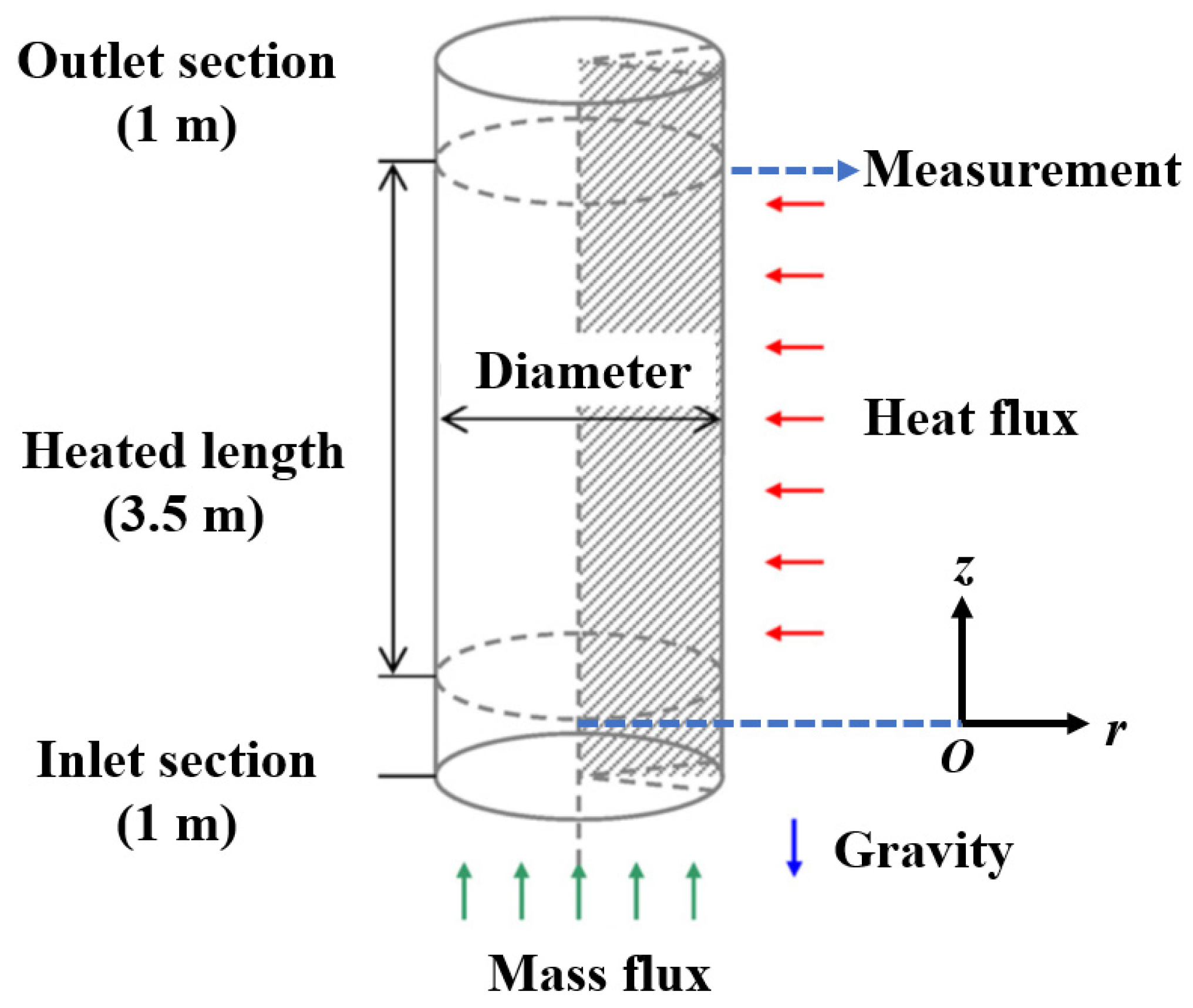
1.4. Experiment Setup and First Loop of NPP

Confidence in the CFD analysis relies on the validation of the numerical calculations against with the experiment data. For this purpose, parameters in the typical experiment facilities especially for the subcooled boiling flow are illustrated in Table 1. It summarizes the physical properties and nondimensional parameters from various facilities in the SUBO (Subcooled boiling facility) [25,26], DEBORA [6,27,28], Arizona State University (ASU) [20,29], Seoul National University (SNU) [30,31], Purdue University [1,32], respectively. In particular, the first loop of NPP is taken into consideration in which the pressure P = 15.70 MPa. The parameters of the first loop of the NPP are based on the previous reference [28].

Table 1. Typical parameters in various experiment facilities for vertical subcooled boiling flow.

Parameters	SUBO	DEBORA		ASU	SNU	Purdue	First Loop of NPP
Fluid	Water	Freon R12		R-113	Water	Water	Water
Channel	Annulus	Round		Annulus	Annulus	Annulus	Round
Orientation	Vertical	Vertical		Vertical	Vertical	Vertical	Vertical
D/mm	33.6	19.2		34.7	32.3	33.0	10.0
P (MPa)	0.15–0.2	1.46	2.62	0.269	0.1–0.2	0.101	15.70
Q (kW/m2)	370–565	76.2	73.6	79.4–125.9	114.8–320.4	54.0–206.0	1000
G (kg/(m2·s))	1113–2093	2028	1990	565–784	476–1061	497–570	3000
hlg (J/kg)	$~2.70\times$106	$1.16\times$105	$8.59\times$104	$1.32\times$105	$~2.23\times$106	$~2.20\times$106	$9.52\times$105
ΔTsub (K)	19–31	28–44	16–18	30–38	11–21	1–20	~20
ρl/ρg	~848.5	14.9	6.7	79.0	~1178	~1608	6.4
Bo	$1.0\times$${10}^{-4}–2.3\times$10−4	$3.0\times$10−4	$4.0\times$10−4	$8.0\times$${10}^{-4}–11\times$10−4	$1.1\times$${10}^{-4}–1.4\times$10−4	$0.5\times$${10}^{-4}–1.6\times$10−4	$3.6\times$10−4
Reg (dp = 1 mm)	$0.3\times$${10}^3–2.0\times$103	$1.1\times$103	$1.4\times$103	$0.5\times$103	$0.5\times$103	$0.4\times$103	$8.5\times$103
Rel	$1.4\times {10}^5–2.5\times {10}^5$	$2.9\times$105	$3.1\times$105	$5.9\times$104	$5.0\times$104	$4.5\times$104	$4.3\times$105
Jae (ΔTsup = 20 K)	5.2–9.0	0.35	0.23	5.8	24.9	35.5	0.080
Eo (dp = 1 mm)	0.16	1.7	2.4	1.1	0.16	0.15	0.61

where Re_g number and Eo number are calculated with bubble diameter d_p = 1 mm; Ja_e number is obtained with wall superheat ΔT_sup = 20 K, Ja_e = SJa, S = $\frac{1}{1+2.53\times {10}^{-6}{\mathrm{Re}}_{\mathrm{l}}^{1.17}}$ (Situ et al., 2005); first loop of NPP is a high-pressure condition with P = 15.70 MPa.

In Table 1, typical experimental parameters like the working fluid, channel, orientation, equivalent hydraulic diameter D, pressure P, wall heat flux Q, mass flow rate G, and inlet liquid subcooling temperature ΔT_sub greatly differ in various experimental facilities. Hence, the relevant nondimensional numbers need to be introduced. Additionally, the nondimensional numbers for the subcooled boiling flow of the typical experiment facilities including the SUBO, DEBORA, ASU, SNU, and Purdue facility are presented in Table 1. For the wall boiling phenomenon in the vertical subcooled boiling flow, the liquid Reynolds number (Re_l), ratio of two phases (ρ_l/ρ_g), effective Jacob number (Ja_e) and Boiling number (Bo) are most important [8]. Especially, the experiment test case analysis based on the typical experimental facilities are presented in Section 3.1.

1.5. Scope of this Paper

An accurate prediction on the interphase behaviors of the vertical gas-liquid subcooled boiling flow is indispensable for the first loop of the NPP with P = 15.70 MPa. Therefore, the interphase behaviors including the bubble size distribution in the first loop of the NPP are analyzed, evaluated, and validated using various wall boiling models coupled with PBM kernels in this paper. In Section 2, firstly, the EE two-fluid framework in the CFD calculation is briefly introduced; then, the wall boiling models are illustrated, including the model of the active nucleation site density, bubble departure diameter, and bubble departure frequency; in addition, the interfacial force models and PBM kernels such as bubble coalescence and breakup are elaborated. In Section 3, the interphase behaviors including the bubble size distribution for the first loop of the NPP are analyzed, evaluated, and validated. Section 4 comes to the conclusions and remarks on the numerical simulation in the vertical gas-liquid subcooled boiling flow.

2. Models and Setup

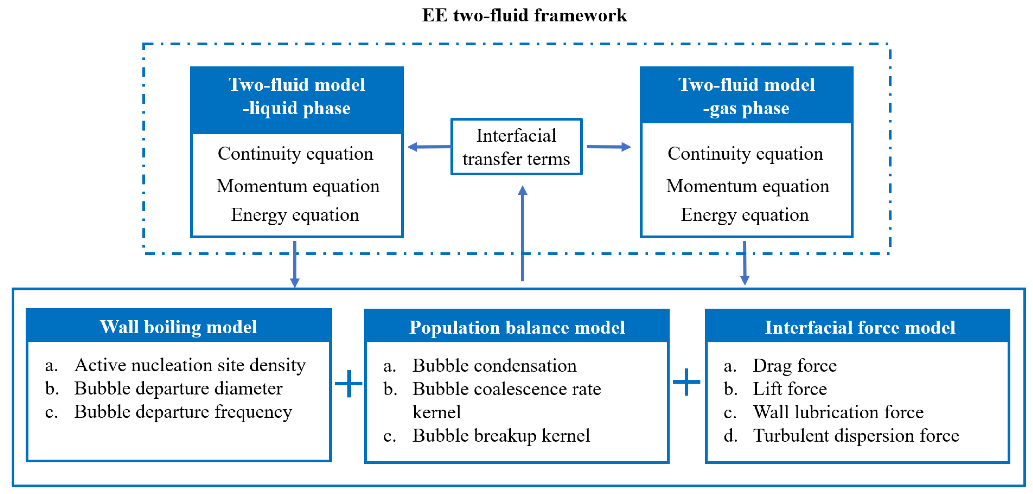
2.1. EE Two-Fluid Framework

Generally, the wall boiling coupled with the PBM model in the EE two-fluid framework for the gas-liquid flow is shown in Figure 1. It consists of the two-fluid model, wall boiling model, PBM kernel and interfacial force model [2,33] which will be described as follows.

Figure 1. Illustration of wall nucleation model coupled with PBM kernel in EE two-fluid framework for gas-liquid flow.

For the wall boiling coupled with the PBM model, the bubble size distribution is described with the population balance equation (PBE) as shown in Equation (3) [16].

$$\frac{\partial n\left(\overrightarrow{x},\overrightarrow{m},t\right)}{\partial t}+\nabla \overrightarrow{x}·\left(\dot{\overrightarrow{x}}n\right)+\nabla \overrightarrow{m}·\left(\dot{\overrightarrow{m}}n\right)=B_{\mathrm{C}}-D_{\mathrm{C}}+B_{\mathrm{B}}-D_{\mathrm{B}}+R_{\mathrm{i}},$$

(3)

where $\overrightarrow{x}$ is the spatial vector; $\overrightarrow{m}$ is the mass of bubbles, kg; t is the time, s; $\dot{\overrightarrow{x}}$ is the time change rate of the bubble physical position; n is the number density of bubbles, 1/m³; $\dot{\overrightarrow{m}}$ is the time change rate of the bubble property (mass or volume) state. Furthermore, B_C, D_C are the source and sink term respectively due to the bubble coalescence, and B_B, D_B are also the source and sink term from the bubble breakup behaviors. Particularly, R_i is the sink term for the bubble condensation.

In addition, the representations of the source and sink term for the bubble coalescence, breakup and condensation with the integrated form are given in Equation (4) [11].

$$\begin{gathered} B_{\mathrm{C}}\left(m\right)=\frac{1}{2}{{\displaystyle \int }}_0^{m}n\left(m-m^{\prime }\right)h\left(m-m^{\prime };m^{\prime }\right)n\left(m^{\prime }\right)\mathrm{d}{m}^{\prime }, \\ {D}_{\mathrm{C}}\left(m\right)={{\displaystyle \int }}_0^{\infty }n\left(m\right)h\left(m;m^{\prime }\right)n\left(m^{\prime }\right)\mathrm{d}{m}^{\prime }, \\ {B}_{\mathrm{B}}\left(m\right)={{\displaystyle \int }}_m^{\infty }n\left(m^{\prime }\right)\Omega \left(m^{\prime }\right)\beta \left(m^{\prime };m\right)\mathrm{d}{m}^{\prime }, \\ {D}_{\mathrm{B}}\left(m\right)=n\left(m\right)\Omega \left(m\right), \end{gathered}$$

(4)

where $n\left(m-m^{\prime }\right)$, $n\left(m^{\prime }\right)$mean the bubbles number density of mass ($m-m^{\prime }$) and $m^{\prime }$ respectively; $h\left(m-m^{\prime };m^{\prime }\right)$ indicates the collision frequency between the bubbles of mass ($m-m^{\prime }$) and $m^{\prime }$; $\Omega \left(m^{\prime }\right)$ represents the overall breakup frequency of the parent bubble with a mass $m^{\prime }$; $\beta \left(m^{\prime };m\right)$ is the daughter bubble size distribution with the parent bubble of a mass $m^{\prime }$.

2.2. Two-Fluid Model

With the treatment of the continua of both the gas and liquid phases, the two-fluid model includes the mass, momentum, and energy equations of each phase in Figure 1. For the closure of the two-fluid model, the interfacial transfer terms are introduced [33,34]. Both the wall boiling model, PBM kernel, and interfacial force model contribute to the interfacial transfer terms, and the two-fluid model is a typical model that was illustrated in many previous research [7,9,14,20]. Consequently, this paper skips the presentations of the equations of the two-fluid model and focuses on the wall boiling and PBM models.

2.3. Wall Boiling Model

For the wall boiling mechanism, the bubble nucleation occurs on the heated wall. Unlike the sink term related with the phase change due to the bubble condensation, the wall boiling model is handled as the boundary condition in Equation (3) [7], and the expression of the wall nucleation interfacial area rate $\Phi$ of the wall boiling model is presented in Equation (5) [2].

$$\Phi =\frac{N_{\mathrm{n}}f{\xi }_{\mathrm{H}}}{A_{\mathrm{C}}}\pi D_{\mathrm{d}}^2,$$

(5)

where ${\xi }_{\mathrm{H}}$ is the heated perimeter of the boiling channel, m; $A_{\mathrm{C}}$ is the cross-sectional area of the boiling channel, m².

As reasonably concluded from Equations (2) and (5), the wall boiling mechanisms include the model of the active nucleation site density $N_{\mathrm{n}}$, bubble departure diameter $D_{\mathrm{d}}$ and bubble departure frequency f. These three models are necessary to compute the wall nucleation interfacial area rate of the wall boiling model. To this end, typical models of the active nucleation site density $N_{\mathrm{n}}$, bubble departure diameter $D_{\mathrm{d}}$ and bubble departure frequency f are summarized in Table 2, Table 3 and Table 4.

2.3.1. Typical Models of Active Nucleation Site Density N_n

Typical models of the active nucleation site density N_n are illustrated in Table 2. In Table 2, firstly, correlation in the form of the power laws depending on the wall superheat ΔT_sup (ΔT_sup = T_w − T_sat) was proposed by Lemmert and Chawla [35]. Then, Kocamustafaogullari and Ishii [36] derived the model of N_n which is highly dependent on the nondimensional cavity radius $R_{\mathrm{c}}^{*}$ and ratio ${\rho }^{*}$ as shown in Equation (6). As the N_n model of Kocamustafaogullari and Ishii [36], it is derived from the pooling boiling condition while it was widely adopted for the subcooled flow boiling condition [37,38,39].

$$\begin{gathered} R_{\mathrm{c}}^{*}=(R_{\mathrm{c}}/(D_{\mathrm{d}}/2\left)\right), \\ {\rho }^{*}=\mathsf{\Delta }\rho /{\rho }_{\mathrm{g}}, \mathsf{\Delta }\rho ({\rho }_{\mathrm{l}}-{\rho }_{\mathrm{g}}), \\ f\left({\rho }^{*}\right)=2.157\times {10}^{-7}{\rho *}^{-3.2}{\left(1+0.0049{\rho }^{*}\right)}^{4.13}, \\ {R}_{\mathrm{c}} = 2\sigma T_{\mathrm{sat}}/({\rho }_{\mathrm{g}}{h}_{\lg }\mathsf{\Delta }{T}_{\mathrm{e}}) \mathrm{for} {\rho }_{\mathrm{g}}\ll {\rho }_{\mathrm{l}} \mathrm{and} h_{\lg }(T_{\mathrm{g}} - T_{\mathrm{sat}})/\left(\mathrm{R}{T}_{\mathrm{g}}{T}_{\mathrm{sat}}\right)\ll 1 \end{gathered}$$

(6)

where R_c is the critical cavity radius based on the wall superheat, m; Δρ is the density difference of the two phases, Δρ = (ρ_l − ρ_g), kg/m³; $f\left({\rho }^{*}\right)$ is the function; ${\rho }^{*}$ is the ratio between the density difference and gas density, ${\rho }^{*}$ = Δρ/${\rho }_{\mathrm{g}}$; σ is the surface tension, N/m; T_sat is the saturation temperature, °C or K; ΔT_e is the effective wall superheat in the gas-liquid flow boiling, ΔT_e = SΔT_sup = S(T_w − T_sat),°C or K; S is the suppression factor in the subcooled convective boiling, 0 < S < 1; T_g is the temperature of the gas phase, °C or K; R is the ideal gas constant, R = 8.3144 J/(K·mol).

Additionally, Basu [40] put forward the model of N_n for the subcooled convective boiling. It is a function of both wall superheat ΔT_sup and contact angle $\theta$. Furthermore, Hibiki and Ishii [21] obtained the model of N_n for both the pool boiling and subcooled convective boiling from the experiment data. It shows that the N_n is a function of the critical cavity radius R_c, contact angle $\theta$ and model parameter ${\rho }^{+}$, ${\rho }^{+}$ =$\log ({\rho }^{*})$. Similarly in Equation (6), R_c = 2$\sigma$T_sat/(${\rho }_{\mathrm{g}}$h_lgΔT_e) for ${\rho }_{\mathrm{g}}\ll {\rho }_{\mathrm{l}}$ and h_lg(T_g − T_sat)/(RT_gT_sat)$\ll$1 in this model. Lastly, a new model with a parametric analysis based on the existing experiment data for the vertical subcooled boiling flow was developed [5]. It is a function of the wall superheat ΔT_sup, pressure P and contact angle $\theta$. And in this model, the additional calculation formulas for the contact angel $\theta$ and pressure P are shown in Equation (7).

$$\begin{gathered} \left(1-\cos \theta \right)=(1-\cos {\theta }_0){\left(\frac{T_{\mathrm{c}}-T_{\mathrm{sat}}}{T_{\mathrm{c}}-T_0}\right)}^{\gamma } \mathrm{for} {\theta }_0 =41.37°, T_{\mathrm{c}} = 374°\mathrm{C}, T_0 = 25°\mathrm{C}, \gamma =0.719, \\ f(P)=26.006-3.678\exp (-2P)-21.907\exp (-\frac{P}{24.065}), \end{gathered}$$

(7)

where θ₀ is the contact angle at the room temperature, °; T₀ is the room temperature, K; T_c is critical temperature at which contact angle becomes 0, °C or K; $\gamma$ is the model parameter.

Table 2. Typical models of active nucleation site density N_n.

Author/Year	Active Nucleation Site Density Nn (1/m2)	Conditions
Lemmert and Chawla, 1977 [35]	Nn= (185ΔTsup)1.805	P = 0.1 − 0.2 MPa; ΔTsup = Tw − Tsat
Kocamustafaogullari and Ishii, 1983 [36]	$N_{\mathrm{nc}}^{*}=R_{\mathrm{c}}^{*}{}^{-4.4}f\left({\rho }^{*}\right)$$, N_{\mathrm{nc}}^{*}=N_{\mathrm{nc}}{D}_{\mathrm{d}}^2$	P = 0.1 − 19.8 MPa; For subcooled flow boiling
Basu et al., 2002 [40]	$N_{\mathrm{nc}}=0.34\times$${10}^4(1-\cos \theta$$)\mathsf{\Delta }{T}_{\sup }^{2.0}$, ΔTONB < ΔTsup < 15 K; $N_{\mathrm{nc}}=3.4\times$${10}^{-1}(1- \cos \theta$$)\mathsf{\Delta }{T}_{\sup }^{5.3}$$, \mathsf{\Delta }{T}_{\sup } \ge$15 K	P = 0.1 − 13.75 MPa; $\theta$ = 0° − 85°; ΔTsub = 1.7 − 80 °C (liquid subcooling temperature); For subcooled flow boiling
Hibiki and Ishii, 2003 [21]	$N_{\mathrm{n}}=\overline{N_{\mathrm{n}}}\left\{1-\exp \left(-\frac{{\theta }^2}{8{\mu }^2}\right)\right\}$ $\left[\exp \left\{f\left({\rho }^{+}\right)\frac{{\lambda }^{\prime }}{R_{\mathrm{c}}}\right\}-1\right]$	P = 0.1 − 19.8 MPa; $N_{\mathrm{n}}=1.0\times$${10}^4-1.51\times$1010 m−2; $\theta$ = 5°–90°; $\overline{N_{\mathrm{n}}}$$=4.72\times$${10}^5 {\mathrm{m}}^{-2}; \mu =0.722 \mathrm{rad}; {\lambda }^{\prime }=2.50\times$10−6 m; For pool boiling and subcooled flow boiling
Li et al., 2018 [5]	$N_{\mathrm{n}}={10}^3 \left(1-\cos \theta \right)$ $\exp \left\{f\left(P\right)\right\}\mathsf{\Delta }{T}_{\sup }^{\left(A\mathsf{\Delta }{T}_{\sup }+B\right)}$	P = 0.1 − 19.8 MPa; A = −0.0002P2 + 0.0108P + 0.0119; B = 0.122P + 1.988; For vertical subcooled flow boiling

where N_nc is active nucleation site density in subcooled convective boiling, m⁻²; $N_{\mathrm{nc}}^{*}$ is nondimensional active nucleation site density in subcooled convective boiling; ΔT_sub is liquid subcooling temperature, ΔT_sub = T_sat − T_l, °C or K; $\overline{N_{\mathrm{n}}}$, $\mu$, ${\lambda }^{\prime }$, A and B are model parameters.

Table 2. Typical models of active nucleation site density N_n.

Author/Year	Active Nucleation Site Density Nn (1/m2)	Conditions
Lemmert and Chawla, 1977 [35]	Nn= (185ΔTsup)1.805	P = 0.1 − 0.2 MPa; ΔTsup = Tw − Tsat
Kocamustafaogullari and Ishii, 1983 [36]	$N_{\mathrm{nc}}^{*}=R_{\mathrm{c}}^{*}{}^{-4.4}f\left({\rho }^{*}\right)$$, N_{\mathrm{nc}}^{*}=N_{\mathrm{nc}}{D}_{\mathrm{d}}^2$	P = 0.1 − 19.8 MPa; For subcooled flow boiling
Basu et al., 2002 [40]	$N_{\mathrm{nc}}=0.34\times$${10}^4(1-\cos \theta$$)\mathsf{\Delta }{T}_{\sup }^{2.0}$, ΔTONB < ΔTsup < 15 K; $N_{\mathrm{nc}}=3.4\times$${10}^{-1}(1- \cos \theta$$)\mathsf{\Delta }{T}_{\sup }^{5.3}$$, \mathsf{\Delta }{T}_{\sup } \ge$15 K	P = 0.1 − 13.75 MPa; $\theta$ = 0° − 85°; ΔTsub = 1.7 − 80 °C (liquid subcooling temperature); For subcooled flow boiling
Hibiki and Ishii, 2003 [21]	$N_{\mathrm{n}}=\overline{N_{\mathrm{n}}}\left\{1-\exp \left(-\frac{{\theta }^2}{8{\mu }^2}\right)\right\}$ $\left[\exp \left\{f\left({\rho }^{+}\right)\frac{{\lambda }^{\prime }}{R_{\mathrm{c}}}\right\}-1\right]$	P = 0.1 − 19.8 MPa; $N_{\mathrm{n}}=1.0\times$${10}^4-1.51\times$1010 m−2; $\theta$ = 5°–90°; $\overline{N_{\mathrm{n}}}$$=4.72\times$${10}^5 {\mathrm{m}}^{-2}; \mu =0.722 \mathrm{rad}; {\lambda }^{\prime }=2.50\times$10−6 m; For pool boiling and subcooled flow boiling
Li et al., 2018 [5]	$N_{\mathrm{n}}={10}^3 \left(1-\cos \theta \right)$ $\exp \left\{f\left(P\right)\right\}\mathsf{\Delta }{T}_{\sup }^{\left(A\mathsf{\Delta }{T}_{\sup }+B\right)}$	P = 0.1 − 19.8 MPa; A = −0.0002P2 + 0.0108P + 0.0119; B = 0.122P + 1.988; For vertical subcooled flow boiling

where N_nc is active nucleation site density in subcooled convective boiling, m⁻²; $N_{\mathrm{nc}}^{*}$ is nondimensional active nucleation site density in subcooled convective boiling; ΔT_sub is liquid subcooling temperature, ΔT_sub = T_sat − T_l, °C or K; $\overline{N_{\mathrm{n}}}$, $\mu$, ${\lambda }^{\prime }$, A and B are model parameters.

2.3.2. Typical Models of Bubble Departure Diameter ${\mathrm{D}}_{\mathrm{d}}$

In the past decades, typical models of the bubble departure diameter $D_{\mathrm{d}}$ are elaborated in Table 3. In Table 3, firstly, correlation in the function of the liquid subcooling temperature ΔT_sub was described by Tolubinsky and Kostanchuk [41]. In 1983, Kocamustafaogullari and Ishii [36] predicted the model of $D_{\mathrm{d}}$ with a wide range of the pressure (P = 0.1 − 19.8 MPa). Then, Situ [4] proposed the nondimensional bubble departure diameter $D_{\mathrm{d}}^{*}$ with a function of the Jacob (Ja) number and Prandtl number (Pr) at the ambient pressure. At last, Krepper [8] derived the model of $D_{\mathrm{d}}$ with the liquid subcooling temperature ΔT_sub in the high-pressure condition. Hence, the model of the bubble departure diameter of Krepper [8] is adopted in this paper.

Table 3. Typical models of bubble departure diameter D_d.

Author/Year	Bubble Departure Diameter Dd	Conditions
Tolubinsky and Kostanchuk, 1970 [41]	$D_{\mathrm{d}}=1.3\times {10}^{-3}\exp \left(\frac{-\mathsf{\Delta }{T}_{\mathrm{sub}}}{53}\right)$	P = 0.1 MPa; For subcooled flow boing
Kocamustafaogullari and Ishii, 1983 [36]	$D_{\mathrm{d}}=0.0012{(\frac{\mathsf{\Delta }\rho }{{\rho }_{\mathrm{g}}})}^{0.9}{D}_{\mathrm{dF}}$$, D_{\mathrm{dF}}$$=0.0208\times \mathsf{\pi }/4\times \sqrt{\sigma }/\sqrt{\mathrm{g}\left(\mathsf{\Delta }\rho \right)}$	P = 0.1 − 19.8 MPa; For pooling boiling
Situ et al., 2005 [4]	$D_{\mathrm{d}}^{*}=\sqrt{C_{\mathrm{l}}}\left(\frac{{\mathrm{j}}_{\mathrm{r}}{D}_{\mathrm{d}}}{{\mu }_{\mathrm{l}}}\right)$$, D_{\mathrm{d}}^{*}=\frac{4\sqrt{\raisebox{1ex}{$22$}\!\left/ \!\raisebox{-1ex}{$3$}\right.}{b}^2}{\pi }{\mathrm{Ja}}_{\mathrm{e}}^2{\mathrm{Pr}}_{\mathrm{l}}^{-1}$	P = 0.1 MPa; $C_{\mathrm{l}}=3.877{\mathrm{j}}_{\mathrm{s}}^{1/2}{\left({\mathrm{Re}}_{\mathrm{g}}^{-2}+0.014{\mathrm{j}}_{\mathrm{s}}^2\right)}^{1/4}$; ${\mathrm{j}}_{\mathrm{s}}=\left|\frac{\mathrm{d}{j}_{\mathrm{l}}}{\mathrm{d}x}\right|\frac{0.5d_{\mathrm{p}}}{j_{\mathrm{r}}}$; b = 1.73; For subcooled flow boing
Krepper et al., 2013 [8]	$D_{\mathrm{d}}=6\times {10}^{-4}\exp \left(\frac{-\mathsf{\Delta }{T}_{\mathrm{sub}}}{45}\right)$	High pressure; For subcooled flow boing

where C_l is shear lift coefficient; D_dF is the departure diameter with Fritz equation, m; g is gravity acceleration, g = 9.80 m/s²; C_Pl is specific heat capacity of liquid phase at a certain pressure, J/(kg·K); j_l is superficial liquid velocity, m/s; j_r is relative velocity between two phases, m/s; j_s is nondimensional fluid velocity gradient; Re_g, bubble Reynolds number; Ja_e, effective Jakob number, Ja_e = SJa = ${\rho }_{\mathrm{l}}$ C_Pl Δ T_e/(${\rho }_{\mathrm{g}}$ h_ig); Pr_l is Prandtl number of liquid phase, Pr_l = C_Plμ_l/k_l; b is model parameter.

Table 3. Typical models of bubble departure diameter D_d.

Author/Year	Bubble Departure Diameter Dd	Conditions
Tolubinsky and Kostanchuk, 1970 [41]	$D_{\mathrm{d}}=1.3\times {10}^{-3}\exp \left(\frac{-\mathsf{\Delta }{T}_{\mathrm{sub}}}{53}\right)$	P = 0.1 MPa; For subcooled flow boing
Kocamustafaogullari and Ishii, 1983 [36]	$D_{\mathrm{d}}=0.0012{(\frac{\mathsf{\Delta }\rho }{{\rho }_{\mathrm{g}}})}^{0.9}{D}_{\mathrm{dF}}$$, D_{\mathrm{dF}}$$=0.0208\times \mathsf{\pi }/4\times \sqrt{\sigma }/\sqrt{\mathrm{g}\left(\mathsf{\Delta }\rho \right)}$	P = 0.1 − 19.8 MPa; For pooling boiling
Situ et al., 2005 [4]	$D_{\mathrm{d}}^{*}=\sqrt{C_{\mathrm{l}}}\left(\frac{{\mathrm{j}}_{\mathrm{r}}{D}_{\mathrm{d}}}{{\mu }_{\mathrm{l}}}\right)$$, D_{\mathrm{d}}^{*}=\frac{4\sqrt{\raisebox{1ex}{$22$}\!\left/ \!\raisebox{-1ex}{$3$}\right.}{b}^2}{\pi }{\mathrm{Ja}}_{\mathrm{e}}^2{\mathrm{Pr}}_{\mathrm{l}}^{-1}$	P = 0.1 MPa; $C_{\mathrm{l}}=3.877{\mathrm{j}}_{\mathrm{s}}^{1/2}{\left({\mathrm{Re}}_{\mathrm{g}}^{-2}+0.014{\mathrm{j}}_{\mathrm{s}}^2\right)}^{1/4}$; ${\mathrm{j}}_{\mathrm{s}}=\left|\frac{\mathrm{d}{j}_{\mathrm{l}}}{\mathrm{d}x}\right|\frac{0.5d_{\mathrm{p}}}{j_{\mathrm{r}}}$; b = 1.73; For subcooled flow boing
Krepper et al., 2013 [8]	$D_{\mathrm{d}}=6\times {10}^{-4}\exp \left(\frac{-\mathsf{\Delta }{T}_{\mathrm{sub}}}{45}\right)$	High pressure; For subcooled flow boing

where C_l is shear lift coefficient; D_dF is the departure diameter with Fritz equation, m; g is gravity acceleration, g = 9.80 m/s²; C_Pl is specific heat capacity of liquid phase at a certain pressure, J/(kg·K); j_l is superficial liquid velocity, m/s; j_r is relative velocity between two phases, m/s; j_s is nondimensional fluid velocity gradient; Re_g, bubble Reynolds number; Ja_e, effective Jakob number, Ja_e = SJa = ${\rho }_{\mathrm{l}}$ C_Pl Δ T_e/(${\rho }_{\mathrm{g}}$ h_ig); Pr_l is Prandtl number of liquid phase, Pr_l = C_Plμ_l/k_l; b is model parameter.

2.3.3. Typical Models of Bubble Departure Frequency f

As shown in Table 4, the expression of the bubble departure frequency f was proposed with multiple parameters [42]. A formula for f by considering the effects of buoyancy, drag and thermodynamics was given [43]. Then, f was derived when the heat flux is low and the bubbles do not noticeably influence with each other [44] in the subcooled boiling. Furthermore, the expression of f was presented in combination with the study of bubble number density in the subcooled boiling [45]. In addition, f was obtained based on the interphase heat flux q and the latent heat of the phase change h_lg [46]. It was already validated with many experiment data sets. In this paper, the model of the bubble departure frequency of Brooks and Hibiki [46] is carried out for the calculation.

Table 4. Typical models of bubble departure frequency f.

Author/Year	Bubble Departure Frequency f	Conditions
Hatton and Hall, 1966 [42]	$f=\frac{3}{\pi {\eta }_{\mathrm{l}}}{[\frac{16k_{\mathrm{l}}\sigma T_{\mathrm{sat}}}{{(h_{\lg }{\rho }_{\mathrm{g}})}^2{D}_{\mathrm{d}}{R}_{\mathrm{c}}}]}^2$	~
Ivey, 1967 [43]	$f=0.9{(\frac{\mathrm{g}}{D_{\mathrm{d}}})}^{0.5}$	Dd > 5 mm at medium and high heat fluxes; 1 mm < Dd < 5 mm at high heat fluxes
Stephan, 1992 [44]	$f=\frac{1}{\pi }\sqrt{\frac{\mathrm{g}}{2D_{\mathrm{d}}}}{[1+\frac{4\sigma }{D_{\mathrm{d}}^2{\rho }_{\mathrm{l}}\mathrm{g}}]}^{0.5}$	P = 0.1 MPa
Kocamustafaogullari and Ishii, 1995 [45]	$f=\frac{1.18}{D_{\mathrm{d}}}{[\frac{\sigma \mathrm{g}\mathsf{\Delta }\rho }{{\rho }_{\mathrm{l}}^2}]}^{0.25}$	Derived from the interfacial area transport equation
Brooks and Hibiki, 2015 [46]	$f=10.7\times \frac{\alpha }{D_{\mathrm{d}}^2}{(\frac{q{D}_{\mathrm{d}}}{\alpha {\rho }_{\mathrm{g}}{h}_{\lg }})}^{0.634}$	3.85 mm < D < 39.2 mm; 5.56 < f < 39.2

where η_l is liquid thermal diffusivity, m²/s; D is hydraulic equivalent diameter, m.

Table 4. Typical models of bubble departure frequency f.

Author/Year	Bubble Departure Frequency f	Conditions
Hatton and Hall, 1966 [42]	$f=\frac{3}{\pi {\eta }_{\mathrm{l}}}{[\frac{16k_{\mathrm{l}}\sigma T_{\mathrm{sat}}}{{(h_{\lg }{\rho }_{\mathrm{g}})}^2{D}_{\mathrm{d}}{R}_{\mathrm{c}}}]}^2$	~
Ivey, 1967 [43]	$f=0.9{(\frac{\mathrm{g}}{D_{\mathrm{d}}})}^{0.5}$	Dd > 5 mm at medium and high heat fluxes; 1 mm < Dd < 5 mm at high heat fluxes
Stephan, 1992 [44]	$f=\frac{1}{\pi }\sqrt{\frac{\mathrm{g}}{2D_{\mathrm{d}}}}{[1+\frac{4\sigma }{D_{\mathrm{d}}^2{\rho }_{\mathrm{l}}\mathrm{g}}]}^{0.5}$	P = 0.1 MPa
Kocamustafaogullari and Ishii, 1995 [45]	$f=\frac{1.18}{D_{\mathrm{d}}}{[\frac{\sigma \mathrm{g}\mathsf{\Delta }\rho }{{\rho }_{\mathrm{l}}^2}]}^{0.25}$	Derived from the interfacial area transport equation
Brooks and Hibiki, 2015 [46]	$f=10.7\times \frac{\alpha }{D_{\mathrm{d}}^2}{(\frac{q{D}_{\mathrm{d}}}{\alpha {\rho }_{\mathrm{g}}{h}_{\lg }})}^{0.634}$	3.85 mm < D < 39.2 mm; 5.56 < f < 39.2

where η_l is liquid thermal diffusivity, m²/s; D is hydraulic equivalent diameter, m.

2.4. Population Balance Model

Different mechanisms including the bubble condensation, bubble coalescence, and breakup are considered in the PBM model when the bubbles enter and leave a control volume in the gas-liquid subcooled flow [23]. The details mechanisms are illustrated below.

2.4.1. Bubble Condensation Model

The bubble condensation model concerns with the sink term of the PBM as shown in Equation (8), and the interphase heat transfer coefficient h is proportional to the Nusselt number (Nu) in Equation (8). Hence, the sink term $R_{\mathrm{i}}$ due to the bubble condensation is mainly determined by the interface area concentration a_i and Nu number. In addition, there are many models of the interface area concentration a_i [47,48,49] and Nu number [50,51,52].

$$\begin{gathered} R_{\mathrm{i}}=-\frac{1}{{\rho }_{\mathrm{g}}\alpha }\frac{h{a}_{\mathrm{i}}\left(T_{\mathrm{sat}}-T_{\mathrm{l}}\right)}{h_{\lg }}{n}_{\mathrm{i}}, \\ h=\frac{\mathrm{Nu}{k}_{\mathrm{l}}}{d_{\mathrm{sm}}}, \end{gathered}$$

(8)

where α is the void fraction; n_i is the number density of bubbles in the discrete bubble class i, m⁻³; d_sm is the Saturn mean diameter, m.

Among them, the models of a_i derived by Kocamustafaogullari [47] and Nu number proposed with Tomiyama [52] in Equation (9) is most applicable for the high-pressure condition [11]. Hence, the two models are adopted for the bubble condensation in the gas-liquid subcooled boiling flow in this paper.

$$\begin{gathered} a_{\mathrm{i}}=\frac{8.49}{D^{0.44}}{(\frac{\sigma }{{\rho }_{\mathrm{l}}})}^{-0.33}{\alpha }^{0.78}{\epsilon }^{0.78} \mathrm{with} \mathrm{high} \mathrm{pressure}, \\ \mathrm{Nu}=2+0.15{\mathrm{Re}}_{\mathrm{g}}^{0.8}{\mathrm{Pr}}_{\mathrm{l}}^{1/2}, \end{gathered}$$

(9)

where ε is the turbulent dissipation rate, m²/s³.

2.4.2. Typical Kernels of Bubble Coalescence

Typical kernels of the a bubble coalescence rate a(d_i, d_j) are illustrated in Table 5 [53,54,55,56,57]. As the bubble coalescence at a collision with a probability, a(d_i, d_j) is represented as the product of the collision frequency h(d_i, d_j) and coalescence efficiency λ(d_i, d_j) in Equation (10) [24]. At the same time, λ(d_i, d_j) is described as the ratio of the time required for coalescence of bubbles t_ij and contact time for two bubbles τ_ij in Equation (10) with various kernels from Table 5. Considering the coalescence rate kernel of Guo [57] includes four collision frequency mechanisms, it is most comprehensive and will be focused on in this paper.

$$\begin{gathered} a(d_{\mathrm{i}}, d_{\mathrm{j}})=h(d_{\mathrm{i}}, d_{\mathrm{j}})\lambda (d_{\mathrm{i}},d_{\mathrm{j}}), \\ \lambda (d_{\mathrm{i}},d_{\mathrm{j}})=\exp (-t_{\mathrm{ij}}/{\tau }_{\mathrm{ij}}), \end{gathered}$$

(10)

where d_i, d_j is diameter of two colliding bubbles, m.

Table 5. Typical kernels of bubbles coalescence rate.

Author/Year	Collision Frequency h(di, dj)	Coalescence Efficiency λ(di, dj)
Prince and Blanch, 1990 [53]	$h(d_{\mathrm{i}},d_{\mathrm{j}})=c_1{(d_{\mathrm{i}}+d_{\mathrm{j}})}^2{(d_{\mathrm{i}}^{\frac{2}{3}}+d_{\mathrm{j}}^{\frac{2}{3}})}^{\frac{1}{2}}{\epsilon }^{\frac{1}{3}}$	$\lambda (d_{\mathrm{i}},d_{\mathrm{j}})=\exp [-c_2\frac{{\rho }_{\mathrm{l}}^{1/2}{\left(\frac{d_{\mathrm{ij}}}{2}\right)}^{5/6}{\epsilon }^{1/3}}{{\sigma }^{1/2}}$]
Luo, 1993 [54]	$h(d_{\mathrm{i}},d_{\mathrm{j}})=c_3(d_{\mathrm{i}}^2+d_{\mathrm{j}}^2){(d_{\mathrm{i}}^{\frac{2}{3}}+d_{\mathrm{j}}^{\frac{2}{3}})}^{\frac{1}{2}}{\epsilon }^{\frac{1}{3}}$	λ(di, dj) = $\exp [-\frac{{(0.75\left(1+{\xi }_{\mathrm{ij}}^2\right)\left(1+{\xi }_{\mathrm{ij}}^3\right))}^{\frac{1}{2}}}{\left(\frac{{\rho }_{\mathrm{g}}}{{\rho }_{\mathrm{l}}}+0.5\right)\left(1+{\xi }_{\mathrm{ij}}^3\right)}{\mathrm{we}}_{\mathrm{ij}}^{\frac{1}{2}}]$
Hibiki and Ishii, 2002 [55]	$h(d_{\mathrm{i}},d_{\mathrm{j}})=c_4\frac{\alpha {\epsilon }^{1/3}}{{\alpha }_{\max }-\alpha }{(\frac{d_{\mathrm{ij}}}{2})}^{-2/3}$	$\mathsf{\lambda }(d_{\mathrm{i}},d_{\mathrm{j}})=\exp [-c_5\frac{{\rho }_{\mathrm{l}}^{\frac{1}{2}}{\left(\frac{d_{\mathrm{ij}}}{2}\right)}^{\frac{5}{6}}{\epsilon }^{\frac{1}{3}}}{{\sigma }^{\frac{1}{2}}}]$
Wang et al., 2005 [56]	$h(d_{\mathrm{i}},d_{\mathrm{j}})=c_6\frac{{\alpha }_{\max }}{{\alpha }_{\max }-\alpha }{\Gamma }_{\mathrm{ij}}{\left(d_{\mathrm{i}}+d_{\mathrm{j}}\right)}^2$ ${(d_{\mathrm{i}}^{\frac{2}{3}}+d_{\mathrm{j}}^{\frac{2}{3}})}^{\frac{1}{2}}{\epsilon }^{\frac{1}{3}}$	λ(di, dj) = $\exp \left[-\frac{{(0.75\left(1+{\xi }_{\mathrm{ij}}^2\right)\left(1+{\xi }_{\mathrm{ij}}^3\right))}^{\frac{1}{2}}}{\left(\frac{{\rho }_{\mathrm{g}}}{{\rho }_{\mathrm{l}}}+\gamma \right)\left(1+{\xi }_{\mathrm{ij}}^3\right)}{\mathrm{we}}_{\mathrm{ij}}^{1/2}\right]$
Guo et al., 2016 [57]	h(di, dj) = h(di, dj)T + h(di, dj)B + h(di, dj)W + h(di, dj)V	$\mathsf{\lambda }(d_{\mathrm{i}},d_{\mathrm{j}})=\exp [-c_2\frac{{\rho }_{\mathrm{l}}^{1/2}{\left(\frac{d_{\mathrm{ij}}}{2}\right)}^{5/6}{\epsilon }^{1/3}}{{\sigma }^{1/2}}]$

where c₁~c₆ are coefficients in coalescence rate kernels, c₁ = 0.28~1.11, c₂ = 0.25ln(h_i/h_f) = 2.3, c₃ = 1.12, c₄ = 0.0157, c₅ = 1.29, c₆ = 1.11; μ_l is dynamic viscosity of liquid phase, Pa·s; d_ij is equivalent diameter of two colliding bubbles with unequal size in coalescence kernels, d_ij = (1/r_i + 1/r_j)⁻¹, m; u_crit is critical velocity for coalescence, m/s; u’ is turbulent fluctuating velocity, m/s; α_max is maximum void faction; Γ_ij is ratio of distance between bubbles and bubble turbulent path length; ${\xi }_{\mathrm{ij}}$ is ratio of diameter of bubble i and j; We_ij is equivalent Weber number of two colliding bubbles in coalescence rate model; γ is coefficient of virtual mass, γ = 0.5; We_ij is equivalent Weber number of two colliding bubbles; h(d_i, d_j)^T, h(d_i, d_j)^B, h(d_i, d_j)^W and h(d_i, d_j)^V are collision frequency due to turbulent fluctuation, buoyancy driven, wake entrainment, and viscous shear, m³/s.

2.4.3. Typical Kernels of Bubble Breakup

For decades, typical kernels of the bubble breakup presented in Table 6 [55,57,58,59,60]. In the bubble breakup process, the breakup frequency and daughter size distribution matter [23]. In Table 6, the kernels of the breakup frequency Ω(V_p) and its daughter size distribution β(V_d, V_p) or the dimensionless form of the daughter size distribution β(f_bv, 1) are elaborated. In the previous research [11], it suggests that the breakup kernel of Luo and Svendsen [60] may be suitable to the high-pressure condition. It will be highlighted in the calculation.

Table 6. Typical models of bubble breakup.

Author/Year	Breakup Frequency Ω(Vp)	Daughter Size Distribution β(fbv, 1)
Coulaloglou and Tavlarides, 1977 [58]	$\Omega (V_{\mathrm{p}})=c_1^{\prime }{d}_{\mathrm{p}}^{-\frac{2}{3}}\frac{{\epsilon }^{\frac{1}{3}}}{1+{\alpha }_1}\exp \left[-c_2^{\prime }\times \frac{\sigma {\left(1+{\alpha }_1\right)}^2}{{\rho }_{\mathrm{g}}{\epsilon }^{\frac{2}{3}}{d}_{\mathrm{p}}^{\frac{5}{3}}}\right]$$, \beta (f_{\mathrm{bv}}, 1)=\frac{3m}{\sqrt{2}\pi }\exp [-\frac{{\left(f_{\mathrm{bv}}-0.5\right)}^2-{\left(3m\right)}^2}{2}]$
Lee et al., 1987 [59]	$\Omega (V_{\mathrm{p}})=c_3^{\prime }{d}_{\mathrm{p}}^{-\frac{2}{3}}{\epsilon }^{\frac{1}{3}}\left[1-\frac{1}{d_{\mathrm{p}}}{{\displaystyle \int }}_0^{d_{\mathrm{p}}}F(\frac{c_4^{\prime }{d}_{\mathrm{p}}^2\sigma }{{\rho }_{\mathrm{l}}{\epsilon }^{\frac{2}{3}}{d}_{\mathrm{ed}}^{\frac{11}{3}}})\mathrm{d}\left(d_{\mathrm{ed}}\right)\right]$$, \beta (f_{\mathrm{bv}}, 1)=\frac{\Gamma \left(a+b\right)}{\Gamma \left(a\right)\Gamma \left(b\right)}{f}_{\mathrm{bv}}^{a-1}{\left(1-f_{\mathrm{bv}}\right)}^{b-1}$
Luo and Svendsen, 1996 [60]	$\Omega (V_{\mathrm{p}}, V_{\mathrm{d}})=0.923\left(1-\alpha \right){(\frac{\epsilon }{d_{\mathrm{p}}^2})}^{\frac{1}{3}}{{\displaystyle \int }}_{{\xi }_{\min }}^1\frac{{\left(1+\xi \right)}^2}{{\xi }^{\frac{11}{3}}}\exp \left[-\frac{12C_{\mathrm{f}}\sigma }{c_5^{\prime }{\rho }_{\mathrm{l}}{\epsilon }^{2/3}{d}_{\mathrm{p}}^{5/3}{\xi }^{11/3}}\right]\mathrm{d}\xi$$, \mathrm{and} \Omega (V_{\mathrm{p}})={{\displaystyle \int }}_0^{0.5}\Omega \left(V_{\mathrm{p}}, V_{\mathrm{d}}\right)\mathrm{d}{f}_{\mathrm{bv}}$$, \beta (f_{\mathrm{bv}}, 1)=\frac{2{{\displaystyle \int }}_{{\xi }_{\min }}^1\frac{{\left(1+\xi \right)}^2}{{\xi }^{\frac{11}{3}}}\exp \left[-\frac{12C_{\mathrm{f}}\sigma }{c_5^{\prime }{\rho }_{\mathrm{l}}{\epsilon }^{2/3}{d}_{\mathrm{p}}^{5/3}{\xi }^{11/3}}\right]\mathrm{d}\xi }{{{\displaystyle \int }}_0^1{{\displaystyle \int }}_{{\xi }_{\min }}^1\frac{{\left(1+\xi \right)}^2}{{\xi }^{\frac{11}{3}}}\exp \left[-\frac{12C_{\mathrm{f}}\sigma }{c_5^{\prime }{\rho }_{\mathrm{l}}{\epsilon }^{2/3}{d}_{\mathrm{p}}^{5/3}{\xi }^{11/3}}\right]\mathrm{d}\xi \mathrm{d}{f}_{\mathrm{bv}}}$
Hibiki and Ishii, 2002 [55]	$\Omega (V_{\mathrm{p}})=\exp [\frac{-c_6^{\prime }\sigma }{{\rho }_{\mathrm{l}}{\epsilon }^{2/3}{d}_{\mathrm{p}}^{5/3}}$], Binary breakup
Guo et al., 2016 [57]	$\Omega (V_{\mathrm{p}}, V_{\mathrm{d}})=\left(1-\alpha \right){{\displaystyle \int }}_{f_{\mathrm{bv},\min }^{\frac{1}{3}}}^1\left[0.913{(\frac{\epsilon }{d_{\mathrm{p}}^2})}^{\frac{1}{3}}\frac{{\left(1+\xi \right)}^2}{{\xi }^{\frac{11}{3}}}+0.103\frac{{\left(1+\xi \right)}^3}{{\xi }^4}{c}_7^{\prime }\right]\exp \left[-\frac{{\tau }_{\mathrm{critical}}}{{\rho }_{\mathrm{l}}{\left(\epsilon \xi d_{\mathrm{p}}\right)}^{2/3}}\right]\mathrm{d}\xi$ Binary breakup

where $c_1^{\prime }$ ~$c_7^{\prime }$ are coefficients in breakup models, $c_1^{\prime }$ = 0.00481, $c_2^{\prime }$ = 0.08, $c_3^{\prime }$ = 1, $c_4^{\prime }$ = α₂(2π)^5/3, $c_5^{\prime }$ = 2, $c_6^{\prime }$ = 1.59, $c_7^{\prime }$ = 2; d_p is diameter of parent bubble in breakup model, m; α₁ is damping constant, 0.05 ≤ α₁ ≤ 0.3; α₂ is ratio of minimum energy required for bubble breakup to bubble surface energy, 0.1 ≤ α₂ ≤ 0.5; m is number of daughter bubbles in breakup model; f_bv is bubble breakup volume fraction; f_bv,min is minimum bubble breakup volume fraction; d_ed is eddy size in breakup model, m; Γ is gamma function; $\xi$ is ratio of diameter of eddy size and diameter of parent bubble; ${\xi }_{\min }$ is minimum value of $\xi$; C_f is coefficient of surface area; τ_critical is critical stress force, kg/m³; Binary breakup means it assuming binary breakup in kernel.

2.4.4. Numerical Solutions of PBM

As the analytical solutions of the PBM are only valid in quite few special cases, the numerical methods are mostly preferred [61]. Firstly, the average bubble number density transportation (ABND) approach is introduced for its relatively less calculation while it has low accuracy [19,34,62]. Then, the method of moments (MOM) is conducted. It includes the quadrature method of moments (QMOM) approach [63] and direct quadrature method of moments (DQMOM) model [13,64], etc. However, it may lead to the monovariate issues.

In addition, the multiple size group (MUSIG) method [16,31] and hence advanced inhomogeneous MUSIG model [8,65,66] are adopted. Although it has similar principles, the inhomogeneous MUSIG approach demands more computation resources than that of the MUSIG method. With the development of computation ability and trade-off between them, the superior of the MUSIG approach dominates [16]. Hence, the MUSIG method will be carried out in this paper.

2.5. Interfacial Force Model

For the modeling of the interfacial momentum forces, the drag force, lift force, wall lubrication force, and turbulent dispersion force are considered [67]. It integrates with the wall boiling model and PCM kernels as illustrated in Figure 1. These models are presented as follows.

2.5.1. Drag Force

Based on the similarity criterion and the mixed viscosity model, Ishii and Zuber [68] established the relationship of the drag coefficient of the two-phase flow. This relationship was widely used in both fluid particle system and solid particle system. The expression is given as follows:

$$F_D=-\frac{1}{2}{C}_D{\rho }_{\mathrm{l}}\left(u_{\mathrm{g}}-u_{\mathrm{l}}\right)\left|u_{\mathrm{g}}-u_{\mathrm{l}}\right|A_{\mathrm{b}},$$

(11)

where C_D is the drag coefficient; $u_{\mathrm{g}}$ and $u_{\mathrm{l}}$ are the average velocity of the gas phase and liquid phase, respectively, m/s.

2.5.2. Lift Force

In the shear flow or turbulence liquid flow, the lift force functions on bubbles by the velocity gradient and negligible viscosity. On this basis, the lift force model proposed by Tomiyama [69] is adopted in this paper. In addition, the lateral net shear lift force $F_{\mathrm{L}}$ induced by the wake and external shear flow field is expressed as shown in Equation (12). The lift coefficient $C_{\mathrm{L}}$ is mainly related to the Re_g number, $\mathrm{Eo}$ number, and its empirical relationship is given in Equation (12).

$$\begin{gathered} F_{\mathrm{L}}=-C_{\mathrm{L}}{\rho }_{\mathrm{l}}\left(u_{\mathrm{g}}-u_{\mathrm{l}}\right)·\nabla u_{\mathrm{l}}, \\ \{\begin{array}{c}m\mathrm{i}n\left[0.288\tan \mathrm{h}\left(0.121{\mathrm{Re}}_{\mathrm{g}}\right), 0.00105{\mathrm{Eo}}^3-0.0159{\mathrm{Eo}}^2-0.0204\mathrm{Eo}+0.474\right],\\ \mathrm{Eo}<4,\\ 0.00105{\mathrm{Eo}}^3-0.0159{\mathrm{Eo}}^2-0.0204Eo+0.474, 4\le Eo\le 10,\\ -0.29,\mathrm{Eo}>10\end{array} \end{gathered}$$

(12)

2.5.3. Wall Lubrication Force

The wall lubrication force primarily acts in radial direction away from the wall. Compared with that of the liquid phase velocity between the bubble and bulk flow field, the liquid phase velocity within the bubble and wall is smaller. This kind of hydrodynamic pressure difference drives bubble away from the wall. From of the wall lubrication force $F_{\mathrm{W}}$ is shown in Equation (13) [70].

$$\begin{gathered} F_{\mathrm{W}}=[C_{\mathrm{w}1}+C_{\mathrm{w}2}(\frac{d_{\mathrm{p}}}{2y_w})]·\frac{\alpha {\rho }_{\mathrm{l}}{\left|\left(u_{\mathrm{g}}-u_{\mathrm{l}}\right)-\left[{\mathit{n}}_{\mathrm{w}}·\left(u_{\mathrm{g}}-u_{\mathrm{l}}\right)\right]{\mathit{n}}_{\mathrm{w}}\right|}^2}{d_{\mathrm{p}}/2}·{\mathit{n}}_{\mathrm{w}}, \\ {C}_{\mathrm{w}1}=-0.104-0.06\left|u_{\mathrm{g}}-u_{\mathrm{l}}\right|, \\ {C}_{\mathrm{w}2}=0.147, \end{gathered}$$

(13)

where $C_{\mathrm{w}1}$, $C_{\mathrm{w}2}$ are the wall lubrication coefficients; $y_w$ is the distance between the bubble and wall, m; ${{n}}_{\mathrm{w}}$ is the unit outward normal vector on the wall surface.

2.5.4. Turbulent Dispersion Force

In this paper, the turbulent dissipative force model of Burns [71] is adopted to calculate the turbulent dissipative force. It describes the turbulent dissipation force $F_{\mathrm{TD}}$ using Farve-averaged variables in Equation (14).

$$F_{\mathrm{TD}}=C_{\mathrm{TD}}{K}_{\mathrm{TD}}\frac{{\nu }_{\mathrm{g}}}{\sigma }\left(\frac{\nabla {\beta }_{\mathrm{l}}}{{\beta }_{\mathrm{l}}}-\frac{\nabla {\beta }_{\mathrm{g}}}{{\beta }_{\mathrm{g}}}\right)$$

(14)

where $C_{\mathrm{TD}}$ is the turbulent diffusion coefficient, $C_{\mathrm{TD}}$ = 1; $K_{\mathrm{TD}}$ is the empirical constant related with the Schmidt number, $K_{\mathrm{TD}}$ = 90; ${\beta }_{\mathrm{g}}$, ${\beta }_{\mathrm{l}}$ are the gas volume fraction and liquid volume fraction correspondingly.

3. Results and Discussion

In this section, firstly, nondimensional numbers of the first loop of the NPP (P = 15.70 MPa) and DEBORA experiment test cases are analyzed with approximation. Then, various combinations of wall boiling models and PBM kernels are calculated with ANSYS fluent software using User-Defined Functions (UDF). In addition, the bubble size distribution d_p, void fraction α, gas superficial velocity j_g and liquid superficial velocity j_l are evaluated with the experiment test case (DEBORA-1). The model of the bubble departure diameter D_d [8] and bubble departure frequency f [46] are specified for efficiency. It is selected from the explanations in Section 2.3.2 and Section 2.3.3.

3.1. Experiment Test Case for First Loop of NPP

Under high-pressure conditions, the availability of the experimental data are highly limited and experimental work are quite difficult. Furthermore, none of the previous experiments provides a complete description [20]. Then, the subcooled boiling experiment with the refrigerant have great advantages. It can obtain the similar nondimensional number with a relative low system pressure [28]. To compare the first loop of the NPP to typical refrigerant experiments with relatively low pressures, the relevant nondimensional numbers should be similar.

3.1.1. Nondimensional Number Approximation Analysis

As illustrated in Section 1.4, the Re_l number, ratio of two phases ρ_l/ρ_g, Ja_e number and Bo number are most considered for the wall boiling phenomena in the vertical subcooled boiling flow. Commonly, the relevant nondimensional numbers should be better within 1 order of the magnitude (<10 times) [8].

In Table 7, typical parameters including the Re_l number, ratio ρ_l/ρ_g, Ja_e number, Bo number of the DEBORA facility are quite close to that in the first loop of the NPP. For the first loop of the NPP (P = 15.70 MPa), the above 4 nondimensional numbers of the DEBORA facility with P = 2.62 MPa condition are similar with each other (all within 3 times). Other nondimensional numbers like the bubble Reynolds number (Re_g) and Eötvös number (Eo) are also less than 1 order of the magnitude with that in the first loop of the NPP (see Section 1.4). In contrast, the ratio ρ_l/ρ_g, Re_g number and Ja_e number of the SUBO, SNU and Purdue facilities are over 1 order of the magnitude than that in the first loop of the NPP as shown in Table 1 in Section 1.4. Therefore, the numerical calculations are compared and analyzed with the experiment data of the DEBORA facility (P = 2.62 MPa) for the first loop of the NPP (P = 15.70 MPa).

Table 7. Comparison of related nondimensional numbers with DEBORA facility and first loop of NPP.

Parameters	DEBORA-1	First Loop of NPP	Ratio
P (MPa)	2.62	15.70	~
ρl/ρg	6.7	6.4	~1
Bo	$4.0\times$10−4	$3.6\times$10−4	~1
Rel	$3.1\times$105	$4.3\times$105	<2
Jae (ΔTsup = 20 K)	0.23	0.080	<3

3.1.2. Experimental Test Case

The illustration of the DEBORA facility is presented in Figure 2. In Figure 2, the length of the inlet section, heated section and outlet section are 1 m, 3.5 m, and 0.5 m, respectively [28]. Meanwhile, the radial profiles of volume fraction and gas velocities at the end of the head section are measured by the optical probe with the coordinate z = 3.5 m. Moreover, a r–z coordinate system is established in Figure 2. Additionally, the detail parameters are given in Table 1. As explained in Section 3.1.1, the experiment test case of DEBORA-1 (P = 2.62 MPa) is approximate with the first loop of the NPP. Hence, experimental data of the DEBORA-1 of the DEBORA facility are selected for the CFD validation.

Figure 2. Illustration of DEBORA facility (measurement position is at z = 3.5 m).

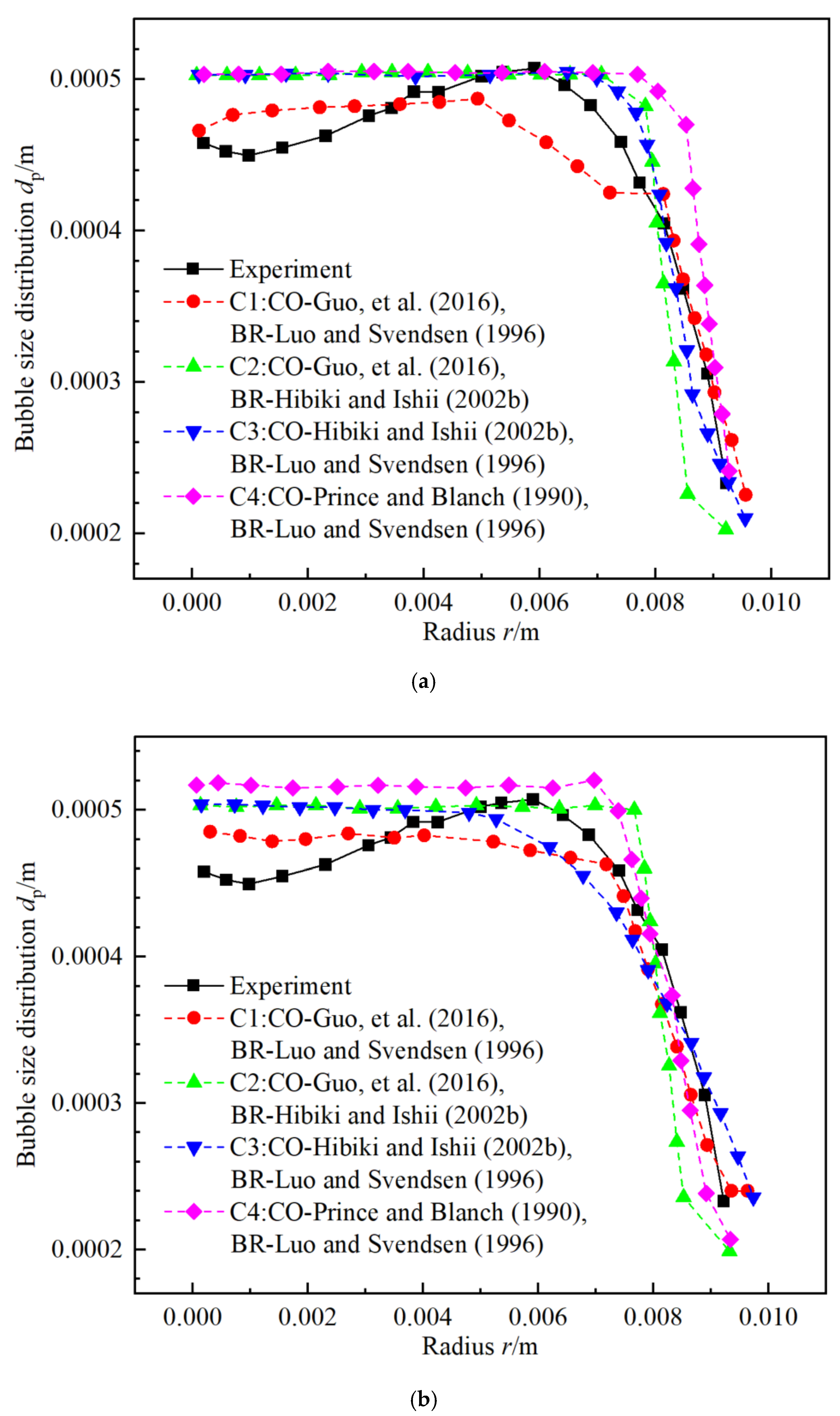
3.2. Analysis of Bubble Size Distribution d_p

In this section, the wall boiling model coupled with the coalescence and breakup kernels are considered for the analysis of the bubble size distribution. Additionally, the calculations of wall boiling models and combinations of coalescence and breakup kernels are analyzed and compared with DEBORA-1 (P = 2.62 MPa) for the first loop of the NPP (P = 15.70 MPa). Before the calculation, the mesh size independencies are carried out. Three mesh sizes of 250,000, 500,000, and 1,000,000 are conducted. For the Sauter mean diameter (SMD) d_p, the former two calculation results are compared with the finest one. Its relative errors of the d_p at the radius r = 0.007 m with z = 3.5 m are 2.9%, 0.2%, respectively. To ensure the accuracy and time, an appropriate mesh size of 500,000 are selected.

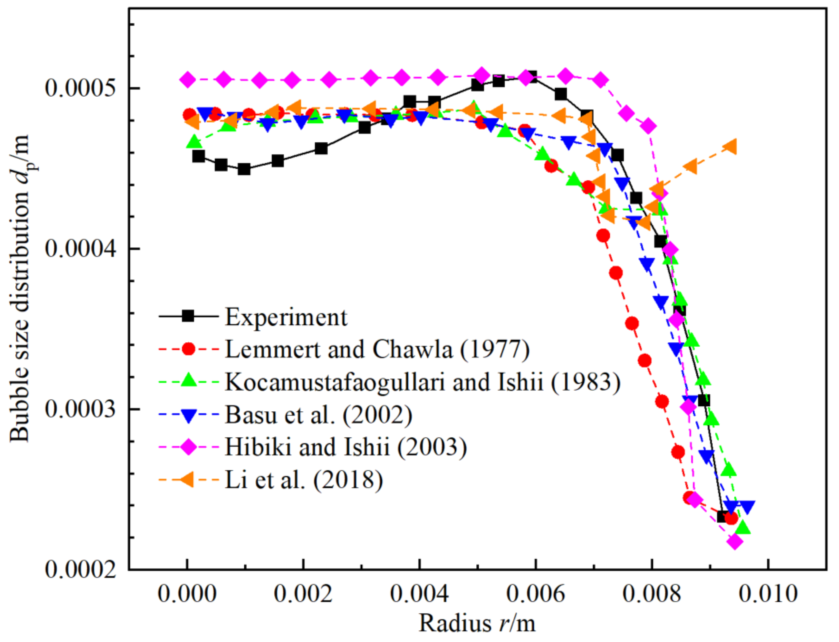
3.2.1. Influence of Wall Boiling Model with DEBORA-1 for First Loop of NPP

For the first loop of NPP, the SMD d_p with various typical models of the active nucleation site density N_n are shown in Figure 3. For the evaluation of the wall boiling models, the coalescence rate kernel of Guo [57] and breakup kernel of Luo and Svendsen [60] are adopted for the PBM model.

Figure 3. Bubble size distribution of SMD d_p of various typical models of N_n with model of D_d [8], f [46], a(d_i, d_j) [57], Ω(V_p), β(f_bv, 1) [54] and DEBORA-1 experiment (P = 2.62 MPa) [28] at z = 3.5 m.

From Figure 3, the maximum relative errors between various models of Lemmert and Chawla [35], Kocamustafaogullari and Ishii [36], Basu [40], Hibiki and Ishii [21], and Li [5] with experiment data from DEBORA-1 are 24.45%, 9.63%, 11.18%, 20.23% and 47.74% respectively. Therefore, the models of Kocamustafaogullari and Ishii [36] and Basu [40] are more accurate than that of Lemmert and Chawla [35], Hibiki and Ishii [21], and Li [5].

3.2.2. Combinations of Coalescence and Breakup Kernel with DEBORA-1 for First Loop of NPP

With the active nucleation site density models of Kocamustafaogullari and Ishii [36] and Basu [40], the SMD d_p with four combinations of coalescence and breakup kernels are conducted in the calculations as shown in Figure 4. In Figure 4a, numerical results of four combinations of C1, C2, C3, and C4 with the N_n model of Kocamustafaogullari and Ishii [36] are obtained. The maximum relative errors between numerical results of C1, C2, C3, and C4 with the DEBORA-1 experiment data are 9.63%, 37.54%, 12.97%, and 29.88%, correspondingly. Consequently, the N_n model of Kocamustafaogullari and Ishii [36] coupled with C1 have better results.

Figure 4. Bubble size distribution of SMD d_p of various combinations of coalescence and breakup kernel with model of D_d [8], f [46] and DEBORA-1 experiment (P = 2.62 MPa) [28] at z = 3.5 m. (a) with N_n of Kocamustafaogullari and Ishii [36], and (b) with N_n of Basu [40].

Similarly in Figure 4b, the maximum relative errors between numerical results of C1, C2, C3, C4 under the N_n model of Basu [40] with the DEBORA-1 experiment data are 11.18%, 34.86%, 25.72%, and 21.99%, respectively. Hence, the N_n model of Basu [40] coupled with C1 performs well. Furthermore, the N_n model of Kocamustafaogullari and Ishii [36] with C1 or Basu [40] with C1 have better performance for the bubble size distribution. Moreover, the N_n model of Kocamustafaogullari and Ishii [36] with C1 performs best in the DEBORA-1 experiment for the first loop of the NPP.

3.2.3. Error Analysis on Bubble Size Distribution

The maximum relative errors of the SMD d_p between numerical results with DEBORA-1 experiment data (P = 2.62 MPa) for the first loop of the NPP (P = 15.70 MPa) is shown in Table 8. For the first loop of the NPP, the N_n model of Kocamustafaogullari and Ishii [36] with C1 (maximum relative error 9.63%) performs better than others.

Table 8. Maximum relative errors between numerical results of d_p with DEBORA-1 experiment data (P = 2.62 MPa) for first loop of NPP (P = 15.70 MPa).

Wall Boiling Model with C1	Maximum Relative Error	Combinations with Kocamustafaogullari and Ishii, 1983	Maximum Relative Error	Combinations with Basu et al., 2002	Maximum Relative Error
Lemmert and Chawla, 1977 [35]	24.45%	C1	9.63%	C1	11.18%
Kocamustafaogullari and Ishii, 1983 [36]	9.63%	C2	37.54%	C2	34.86%
Basu et al., 2002 [40]	11.18%	C3	12.97%	C3	25.72%
Hibiki and Ishii, 2003 [21]	20.23%	C4	29.88%	C4	21.99%
Li et al., 2018 [5]	47.74%	~	~	~	~

On the one hand, the N_n model of Kocamustafaogullari and Ishii [36] relates with the nondimensional cavity radius $R_{\mathrm{c}}^{*}$, wall superheat ΔT_sup and density ratio ${\rho }^{*}$. On the other hand, the N_n model of Basu [40] relies on the wall superheat ΔT_sup and contact angle $\theta$. These two models have more insights into the wall boiling mechanisms for the subcooled boiling flow in the first loop of the NPP.

For the CO kernel of Guo [57], it contains four collision frequency mechanisms and more complete than others. At the same time, the BR kernel of Luo and Svendsen [54] which is based on the BR kernel of Lee [59] are more sophisticated. Therefore, the combinations of C1 (CO-Guo [57] &BR–Luo and Svendsen [54]) with the N_n model of Kocamustafaogullari and Ishii [36] or Basu [40] lead to better results.

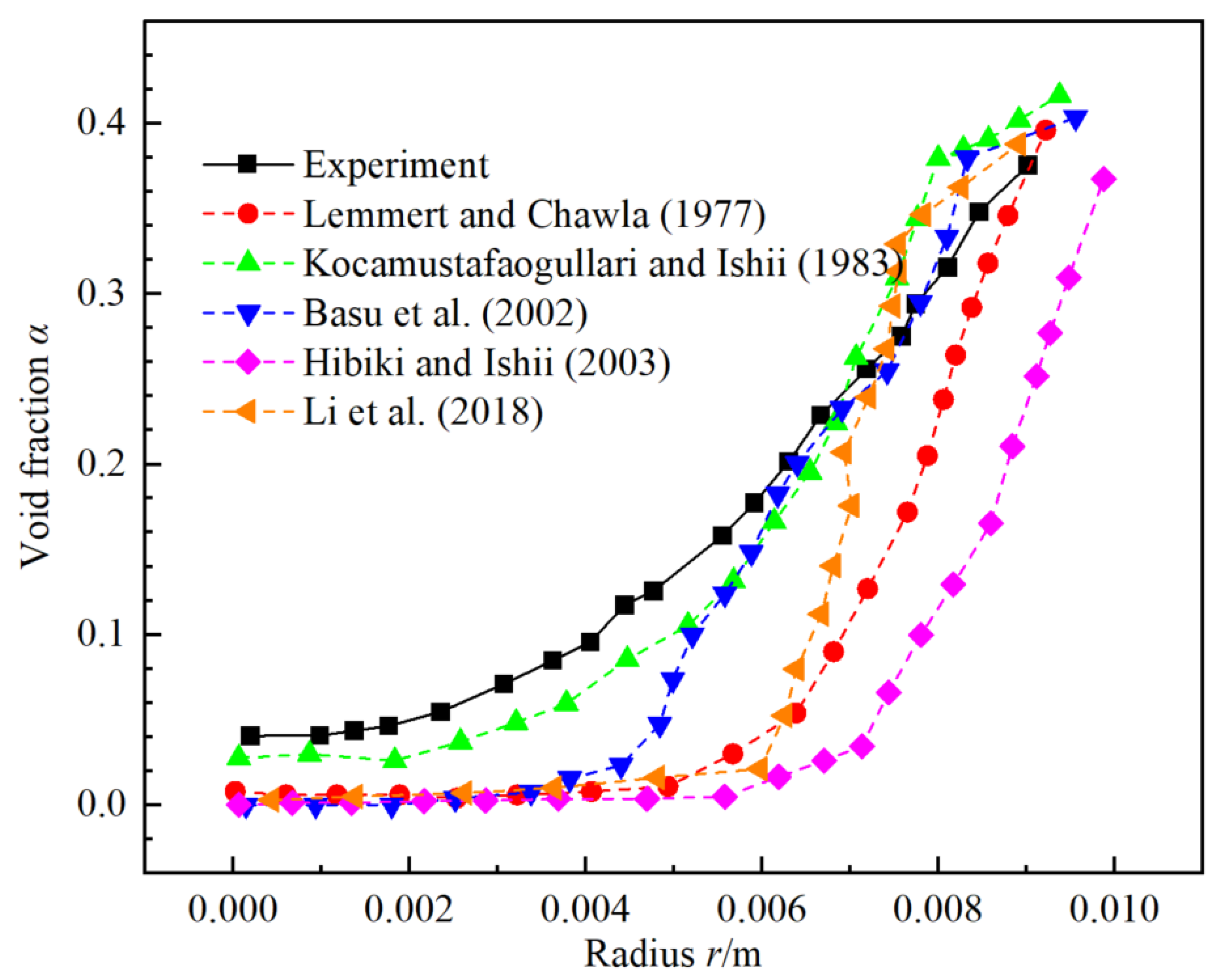
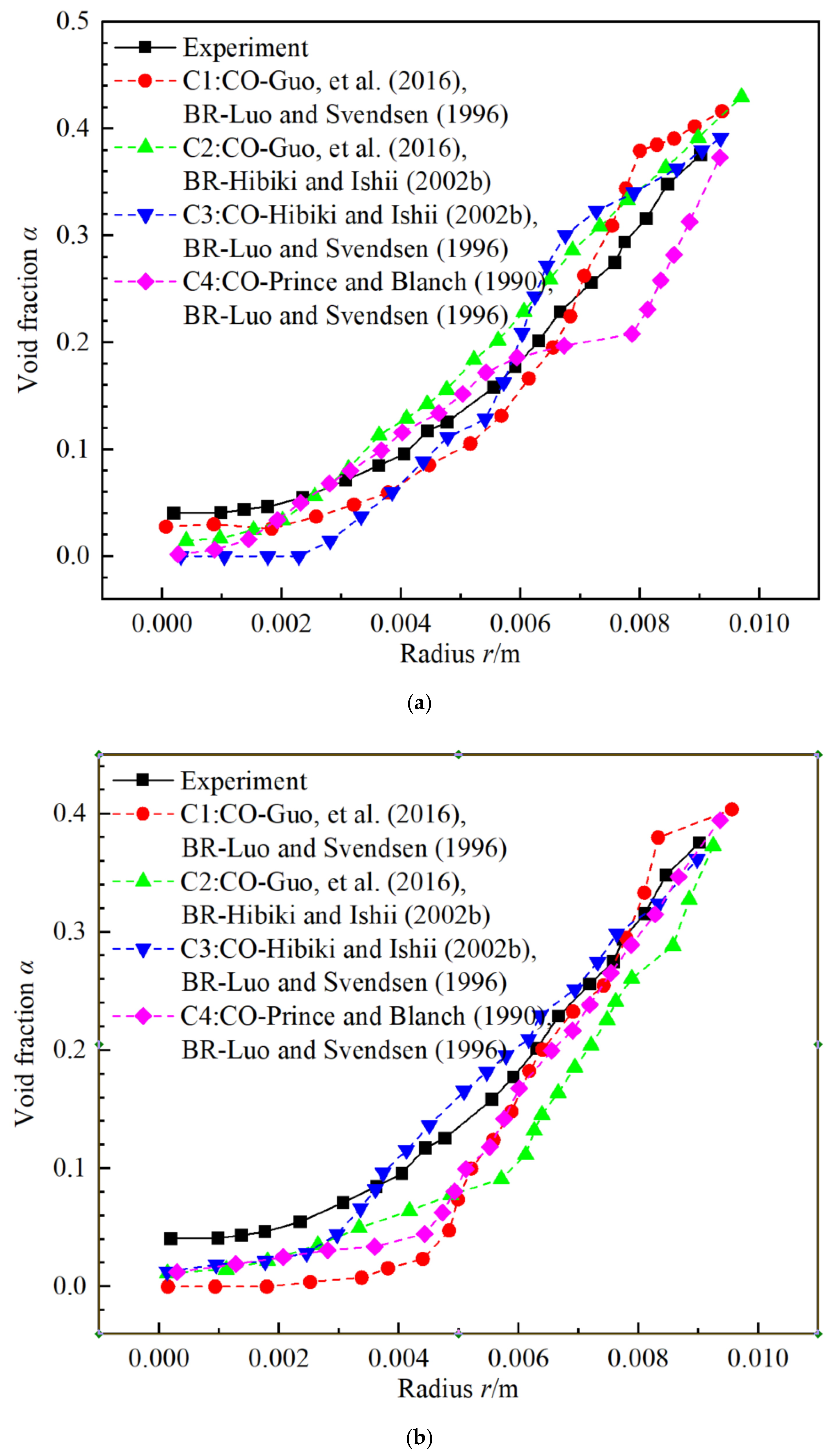
3.3. Calculation of Void Fraction α

Then, the wall boiling model coupled with the coalescence and breakup kernels are adopted for the calculation of the void fraction α in this section. Meanwhile, the influence of wall boiling models and combinations of coalescence and breakup kernels are considered with DEBORA-1 (P = 2.62 MPa) for the first loop of the NPP.

3.3.1. Influence of Wall Boiling Model with DEBORA-1 for First Loop of NPP

For the first loop of the NPP, the void fraction α with various typical models of the active nucleation site density N_n [5,21,35,36,40] are given in Figure 5.

Figure 5. Void fraction α distribution of various typical models of N_n with model of D_d [8], f [46], a(d_i, d_j) [57], Ω(V_p), β(f_bv, 1) [54] and DEBORA-1 experiment (P = 2.62 MPa) [28] at z = 3.5 m.

From Figure 5, the maximum relative errors between various models of Lemmert and Chawla [35], Kocamustafaogullari and Ishii [36], Basu [40], Hibiki and Ishii [21], and Li [5] with experiment data from DEBORA-1 are 96.41%, 29.64%, 80.07%, 90.65%, and 88.03%, respectively. Therefore, the model of Kocamustafaogullari and Ishii [36] are more accurate than that of Lemmert and Chawla [35], Basu [40], Hibiki and Ishii [21] and Li [5].

3.3.2. Combinations of Coalescence and Breakup Kernel with DEBORA-1 for First Loop of NPP

With the active nucleation site density models of Kocamustafaogullari and Ishii [36] and Basu [40], void fraction α with four combinations of coalescence and breakup kernels are conducted in the calculations in Figure 6.

Figure 6. Void fraction α distribution of various combinations of coalescence and breakup kernel with model of D_d [8], f [46] and DEBORA-1 experiment (P = 2.62 MPa) [28] at z = 3.5 m. (a) with Nn of Kocamustafaogullari and Ishii [36], (b) with N_n of Basu [40].

In Figure 6a, the maximum relative errors between four combinations of C1, C2, C3 and C4 under the N_n model of Kocamustafaogullari and Ishii [36] with the DEBORA-1 experiment data are 29.64%, 64.06%, 100.00% and 95.07% correspondingly. Consequently, the N_n model of Kocamustafaogullari and Ishii [36] coupled with C1 has relatively better results. Similarly in Figure 6b, the maximum relative errors between four combinations of C1, C2, C3, C4 under the N_n model of Basu [40] with the experiment data are 100.00%, 72.16%, 68.57%, and 69.82% respectively. Finally, the N_n model of Kocamustafaogullari and Ishii [36] coupled with C1 has nice behaviors.

3.3.3. Error Analysis on Void Fraction α

The maximum relative errors of the void fraction α between numerical results with DEBORA-1 experiment data (P = 2.62 MPa) for the first loop of the NPP (P = 15.70 MPa) is shown in Table 9.

Table 9. Maximum relative errors between numerical results of α with DEBORA-1 experiment data (P = 2.62 MPa) for first loop of NPP (P = 15.70 MPa).

Wall Boiling Model with C1	Maximum Relative Error	Combinations with Kocamustafaogullari and Ishii, 1983	Maximum Relative Error	Combinations with Basu et al., 2002	Maximum Relative Error
Lemmert and Chawla, 1977 [35]	96.41%	C1	29.64%	C1	100.00%
Kocamustafaogullari and Ishii, 1983 [36]	29.64%	C2	64.06%	C2	72.16%
Basu et al., 2002 [40]	80.07%	C3	100.00%	C3	68.57%
Hibiki and Ishii, 2003 [21]	90.65%	C4	95.07%	C4	69.82%
Li et al., 2018 [5]	88.03%	~	~	~	~

For the first loop of the NPP, the N_n model of Kocamustafaogullari and Ishii [36] with C1 (maximum relative error 29.64%) performs best than others. Models of Kocamustafaogullari and Ishii [36] have more insights into the wall boiling mechanisms for the subcooled boiling flow in the first loop of the NPP. Lastly, the combinations of C1 (CO-Guo [57] &BR-Luo and Svendsen [54]) are more complete and fully described than other combinations. This is consistent with that of the bubble size distribution in Section 3.2.3.

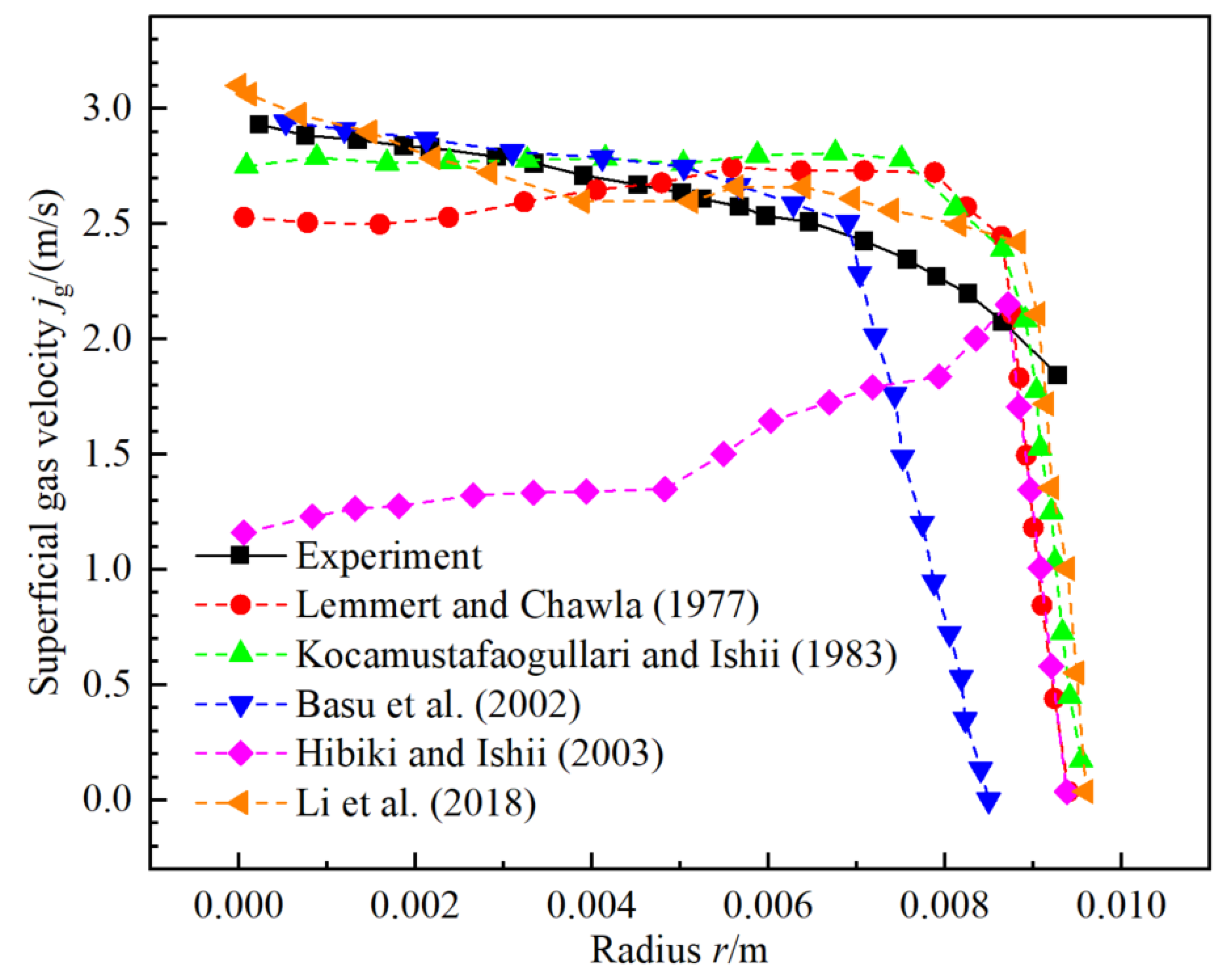
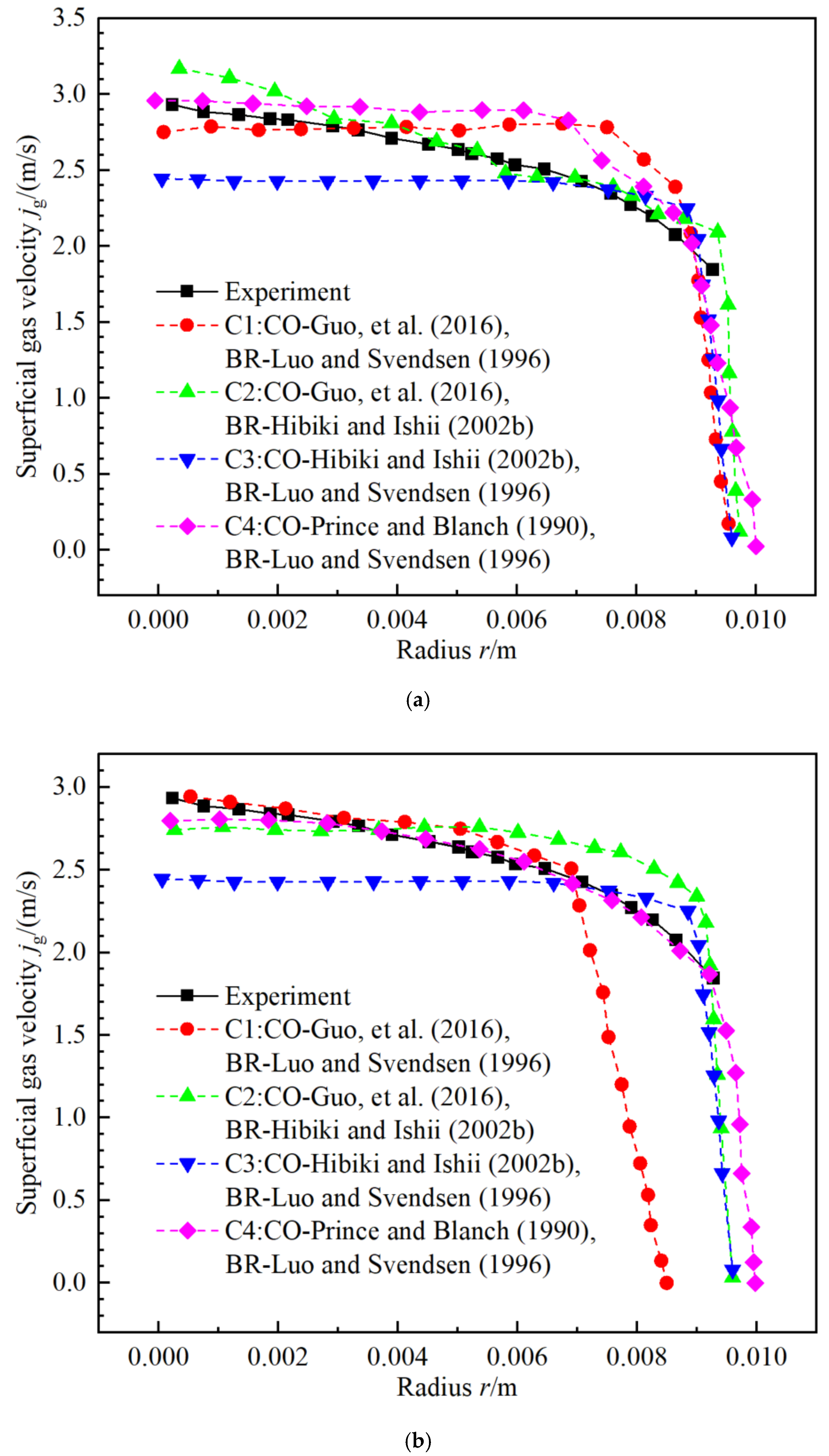
3.4. Comparison of Gas Superficial Velocity j_g

Furthermore, the wall boiling model coupled with the coalescence and breakup kernels are adopted for the calculation of the gas superficial velocity j_g in this section. At the same time, the influence of wall boiling models and combinations of coalescence and breakup kernels are taken into account with DEBORA-1 (P = 2.62 MPa) for the first loop of the NPP (P = 15.70 MPa).

3.4.1. Influence of Wall Boiling Model with DEBORA-1 for First Loop of NPP

For the first loop of the NPP, the gas superficial velocity j_g with various typical models of the active nucleation site density N_n [5,21,35,36,40] are presented in Figure 7.

Figure 7. Superficial gas velocity j_g distribution of various typical models of N_n with model of D_d [8], f [46], a(d_i, d_j) [57], Ω(V_p), β(f_bv, 1) [54] and DEBORA-1 experiment (P = 2.62 MPa) [28] at z = 3.5 m.

From Figure 7, except the near wall region, the maximum relative errors between various models of Lemmert and Chawla [35], Kocamustafaogullari and Ishii [36], Basu [40], Hibiki and Ishii [23] and Li [5] with experiment data from DEBORA-1 are 19.84%, 18.56%, 93.50%, 60.42%, and 13.65%, respectively. Therefore, the models of Kocamustafaogullari and Ishii [36] and Li [5] perform better than other models. To ensure the consistency with the previous analysis, the model of Kocamustafaogullari and Ishii [36] will be focused on as well as the model of Basu [40].

3.4.2. Combinations of Coalescence and Breakup Kernel with DEBORA-1 for First Loop of NPP

The gas superficial velocity j_g with four combinations of coalescence and breakup kernels are conducted in the calculations as given in Figure 8. It is coupled with the N_n models of Kocamustafaogullari and Ishii [36] and Basu [40].

Figure 8. Superficial gas velocity j_g distribution of various combinations of coalescence and breakup kernel with model of D_d [8], f [46] and DEBORA-1 experiment (P = 2.62 MPa) [28] at z = 3.5 m. (a) with Nn of Kocamustafaogullari and Ishii [36], and (b) with N_n of Basu [40].

In Figure 8a, except the near wall region (r > 8.5 mm), the relative errors between four combinations of C1, C2, C3, and C4 under the N_n model of Kocamustafaogullari and Ishii [36] with the experiment data are 18.56%, 8.06%, 16.65%, and 12.77% correspondingly. Thus, the N_n model of Kocamustafaogullari and Ishii [36] coupled with C2 has relatively better results.

As shown in Figure 8b, except the near wall region (r > 8.5 mm), the relative errors between four combinations of C1, C2, C3, and C4 under the N_n model of Basu [40] with the experiment data are 100.00%, 14.74%, 16.65%, and 4.67%, respectively. Hence, the N_n model of Basu [40] coupled with C4 behaves well. In summary, the N_n model of Basu [40] coupled with C4 performs best.

3.4.3. Error Analysis on Gas Superficial Velocity j_g

The maximum relative errors of the gas superficial velocity j_g between numerical results with DEBORA-1 experiment data (P = 2.62 MPa) for the first loop of the NPP (P = 15.70 MPa) is shown in Table 10.

Table 10. Maximum relative errors between numerical results of j_g with DEBORA-1 experiment data (P = 2.62 MPa) for first loop of NPP (P = 15.70 MPa).

Wall Boiling Model with C1	Maximum Relative Error	Combinations with Kocamustafaogullari and Ishii, 1983	Maximum Relative Error	Combinations with Basu et al., 2002	Maximum Relative Error
Lemmert and Chawla, 1977 [35]	19.84%	C1	18.56%	C1	100.00%
Kocamustafaogullari and Ishii, 1983 [36]	18.56%	C2	8.06%	C2	14.74%
Basu et al., 2002 [40]	93.50%	C3	16.65%	C3	16.65%
Hibiki and Ishii, 2003 [21]	60.42%	C4	12.77%	C4	4.67%
Li et al., 2018 [5]	13.65%	~	~	~	~

Considering the calculation of the gas superficial velocity j_g near the wall region is influenced by the wall effect and measurement discrepancy, the error analysis on the gas superficial velocity j_g are mainly except the near wall region. For the first loop of the NPP, the model of Basu [40] coupled with C4 (maximum relative error 4.67%) has nice behaviors.

For the first loop of the NPP, the combination C4 is more suitable than C1 for the calculation of the gas superficial velocity j_g. Compared C4 (CO-Prince and Blanch [53]&BR-Luo and Svendsen [54]) with C1 (CO-Guo [57]&BR-Luo and Svendsen [54]), the breakup kernel is the same while the coalescence kernel differs. For the collision frequency h(d_i, d_j), it is mainly due to four mechanisms: turbulence-induced collision; buoyancy-induced collision; wake-entrainment collision; viscous shear-induced collision. In addition, the coalescence kernel of Prince and Blanch [53] considers the turbulence-induced collision while the coalescence kernel of Guo [57] takes the four mechanisms together. Hence, the results show that the gas superficial velocity j_g could mainly dependent on the turbulence-induced collision which leads to better results.

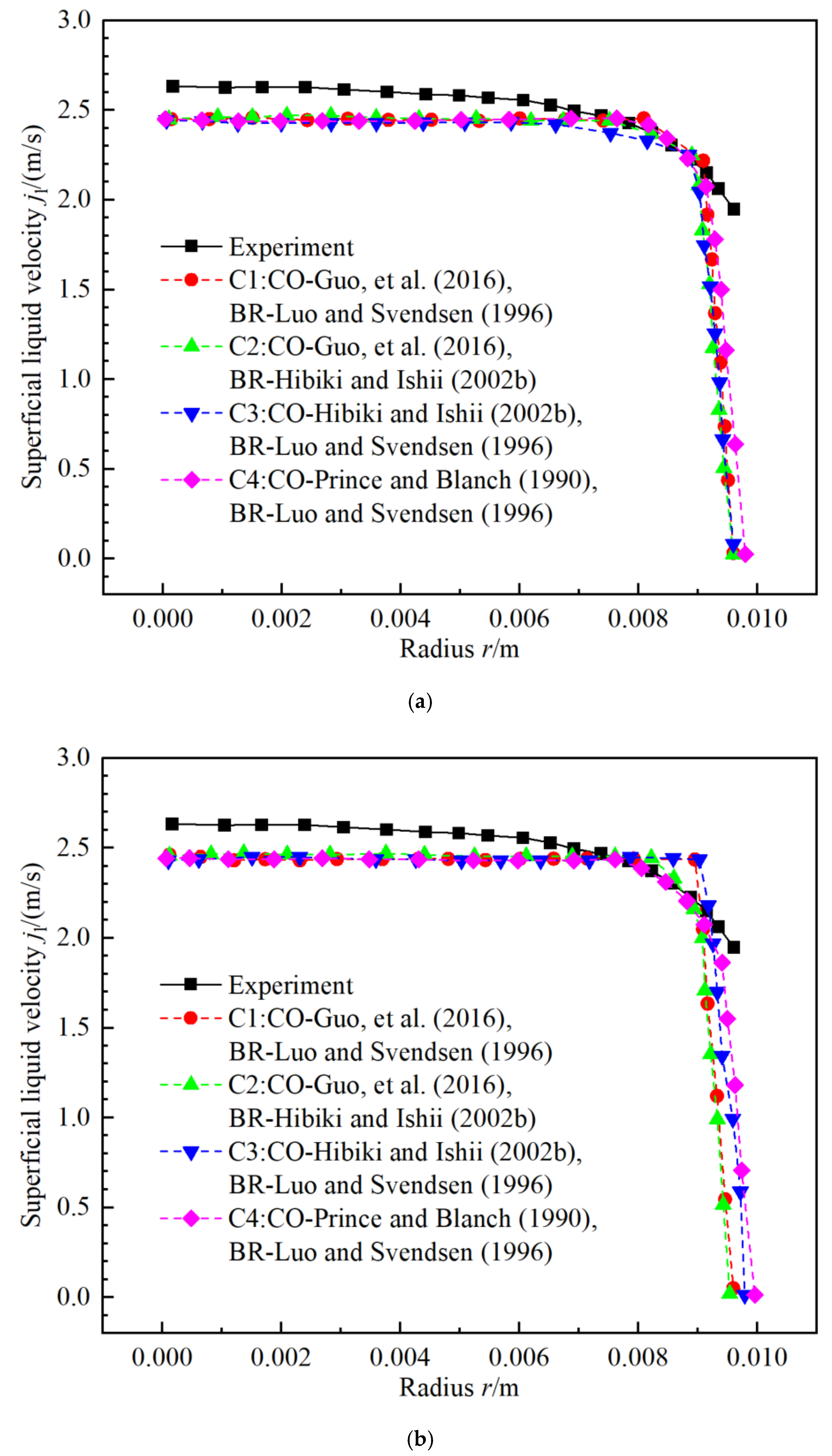
3.5. Tendency of Liquid Superficial Velocity j_l

Lastly, the wall boiling model coupled with the coalescence and breakup kernels are adopted for the calculation of the liquid superficial velocity j_l in this section. In the meantime, the results of wall boiling models and combinations of coalescence and breakup kernels are compared with DEBORA-1 (P = 2.62 MPa) for the first loop of the NPP (P = 15.70 MPa).

3.5.1. Influence of Wall Boiling Model with DEBORA-1 for First Loop of NPP

For the first loop of the NPP, the liquid superficial velocity j_l with various typical models of the active nucleation site density N_n [5,21,35,36,40] are presented in Figure 9.

Figure 9. Superficial liquid velocity j_l distribution of various typical models of N_n with model of D_d [8], f [46], a(d_i, d_j) [57], Ω(V_p), β(f_bv, 1) [54], and DEBORA-1 experiment (P = 2.62 MPa) [28] at z = 3.5 m.

From Figure 9, except the near wall region, the maximum relative errors between various models of Lemmert and Chawla [35], Kocamustafaogullari and Ishii [36], Basu [40], Hibiki and Ishii [21], and Li [5] with experiment data from DEBORA-1 are 25.95%, 6.97%, 6.50%, 28.12%, and 14.43%, respectively. Therefore, the models of Kocamustafaogullari and Ishii [36] and Li [40] perform better than other models.

3.5.2. Combinations of Coalescence and Breakup Kernel with DEBORA-1 for First Loop of NPP

The liquid superficial velocity j_l with four combinations of coalescence and breakup kernels are conducted in the calculations as given in Figure 10. In Figure 10a, except the near wall region (r > 8.5 mm), the maximum relative errors between four combinations of C1, C2, C3, and C4 under the N_n model of Kocamustafaogullari and Ishii [36] with the experiment data are 6.97%, 6.97%, 7.19%, and 6.97%, correspondingly. Thus, the N_n model of Kocamustafaogullari and Ishii [36] coupled with all combinations separately has relatively better results.

Figure 10. Superficial liquid velocity j_l distribution of various combinations of coalescence and breakup kernel with model of D_d [8], f [46] and DEBORA-1 experiment (P = 2.62 MPa) [28] at z = 3.5 m. (a) with N_n of Kocamustafaogullari and Ishii [36], and (b) with N_n of Basu [40].

As shown in Figure 10b, except the near wall region, the maximum relative errors between four combinations of C1, C2, C3, and C4 under the N_n model of Basu et al. (2002) with the experiment data are 6.50%, 6.63%, 7.68%, and 7.21%, respectively. Hence, the N_n model of Basu [40] coupled with all combinations alone behaves well.

3.5.3. Error Analysis on Liquid Superficial Velocity j_l

The maximum relative errors of the liquid superficial velocity j_l between numerical results with DEBORA-1 experiment data (P = 2.62 MPa) for the first loop of the NPP (P = 15.70 MPa) is shown in Table 11.

Table 11. Maximum relative errors between numerical results of j_l with DEBORA-1 experiment data (P = 2.62 MPa) for first loop of NPP (P = 15.70 MPa).

Wall Boiling Model with C1	Maximum Relative Error	Combinations with Kocamustafaogullari and Ishii, 1983	Maximum Relative Error	Combinations with Basu et al., 2002	Maximum Relative Error
Lemmert and Chawla, 1977 [35]	25.95%	C1	6.97%	C1	6.50%
Kocamustafaogullari and Ishii, 1983 [36]	6.97%	C2	6.97%	C2	6.63%
Basu et al., 2002 [40]	6.50%	C3	7.19%	C3	7.68%
Hibiki and Ishii, 2003 [21]	28.12%	C4	6.97%	C4	7.21%
Li et al., 2018 [5]	14.43%	~	~	~	~

Similarly, the liquid superficial velocity j_l near the wall region has large deviations due to the wall effect and measurement discrepancy. Hence, the error analysis in this section excludes the near wall region. For the first loop of the NPP, the N_n model of Basu [40] coupled with C1 (maximum relative error 6.50%) also has nice behaviors.

4. Conclusions

In this work, the wall boiling coupled with the PBM models including the wall nucleation, bubble departure, bubble condensation, coalescence, and breakup are analyzed for the gas-liquid subcooled boiling flow in the first loop of the NPP. Firstly, nondimensional numbers of the first loop of the NPP (P = 15.70 MPa) and experiment test cases DEBORA-1 (P = 2.62 MPa) are analyzed with approximation. Then, five active nucleation site density models coupled with the kernel combination C1 are calculated and analyzed with ANSYS fluent software using UDF. In addition, four combinations of the PBM kernels with the active nucleation site density models of Kocamustafaogullari and Ishii [36] and Basu [40] are evaluated for the first loop of the NPP. Lastly, various behaviors including the bubble size distribution d_p, void fraction α, gas superficial velocity j_g and liquid superficial velocity j_l are compared and validated with the DEBORA-1 (P = 2.62 MPa) of the DEBORA facility. Main conclusions are as below:

• Foremostly, the N_n model the models of Kocamustafaogullari and Ishii [36] and Basu [40] are suitable for the calculations of the subcooled boiling flow in the first loop of the NPP.
• Afterwards, for the bubble size distribution SMD d_p, the N_n model of Kocamustafaogullari and Ishii [36] with C1 (maximum relative error 9.63%) has relatively better behaviors for the first loop of the NPP.
• Then, for the void fraction α, the N_n model of Kocamustafaogullari and Ishii [36] with C1 (maximum relative error 29.64%) performs best than others for the first loop of the NPP.
• Furthermore, for the gas superficial velocity j_g, the model of Basu [40] coupled with C4 (maximum relative error 4.67%) has nice behaviors for the first loop of the NPP.
• Moreover, for the liquid superficial velocity j_l, the N_n model of Basu [40] coupled with C1 coupled with all combinations alone behaves well. In the first loop of the NPP, the N_n model of Basu [40] coupled with C1 (maximum relative error 6.50%) behaves best.
• In addition, the N_n model of Kocamustafaogullari and Ishii [36] relates with the nondimensional cavity radius $R_{\mathrm{c}}^{*}$, wall superheat ΔT_sup and density ratio ${\rho }^{*}$. On the other hand, the N_n model of Basu [40] relies on the wall superheat ΔT_sup and contact angle $\theta$. These two models have more insights into the wall boiling mechanisms for the subcooled boiling flow in the first loop of the NPP.
• Especially, the combination C4 is more suitable than C1 for the calculation of the gas superficial velocity j_g for the first loop of the NPP. The gas superficial velocity j_g could mainly dependent on the turbulence-induced collision which the C4 is mainly related with.
• At last, the CO kernel of Guo [57] contains four collision frequency mechanisms and more complete than others. At the same time, the BR kernel of Luo and Svendsen [54] which is based on the BR kernel of Lee [59] are more sophisticated. Therefore, the combinations of C1 are applicable for the calculation of the bubble size distribution d_p, void fraction α, and liquid superficial velocity j_l.

The results indicate that the detailed evaluation and comparison of the wall boiling coupled with PBM models are particularly crucial for the practical engineering issues. Evaluations on the wall boiling models coupled with PBM kernels are elaborated for the first loop of the NPP (P = 15.70 MPa). In the end, this paper can provide guidance for the numerical computation of the subcooled boiling flow of the first loop of the NPP.

References

- Situ, R.; Ishii, M.; Hibiki, T.; Tu, J.Y.; Yeoh, G.H.; Mori, M. Bubble departure frequency in forced convective subcooled boiling flow. Int. J. Heat Mass Transf. 2008, 51, 6268–6282. [Google Scholar] [CrossRef]
- Chuang, T.-J.; Hibiki, T. Vertical upward two-phase flow CFD using interfacial area transport equation. Prog. Nucl. Energy 2015, 85, 415–427. [Google Scholar] [CrossRef]
- Zhang, R.; Cong, T.; Tian, W.; Qiu, S.; Su, G. Effects of turbulence models on forced convection subcooled boiling in vertical pipe. Ann. Nucl. Energy 2015, 80, 293–302. [Google Scholar] [CrossRef]
- Situ, R.; Hibiki, T.; Ishii, M.; Mori, M. Bubble lift-off size in forced convective subcooled boiling flow. Int. J. Heat Mass Transf. 2005, 48, 5536–5548. [Google Scholar] [CrossRef] [Green Version]
- Li, Q.; Jiao, Y.; Avramova, M.; Chen, P.; Yu, J.; Chen, J.; Hou, J. Development, verification and application of a new model for active nucleation site density in boiling systems. Nucl. Eng. Des. 2018, 328, 1–9. [Google Scholar] [CrossRef]
- Krepper, E.; Končar, B.; Egorov, Y. CFD modelling of subcooled boiling—Concept, validation and application to fuel assembly design. Nucl. Eng. Des. 2007, 237, 716–731. [Google Scholar] [CrossRef]
- Yeoh, G.; Tu, J. Numerical modelling of bubbly flows with and without heat and mass transfer. Appl. Math. Model. 2006, 30, 1067–1095. [Google Scholar] [CrossRef]
- Krepper, E.; Rzehak, R.; Lifante, C.; Frank, T. CFD for subcooled flow boiling: Coupling wall boiling and population balance models. Nucl. Eng. Des. 2013, 255, 330–346. [Google Scholar] [CrossRef]
- Liao, Y.; Lucas, D. Possibilities and limitations of CFD simulation for flashing flow scenarios in nuclear applications. Energies 2017, 10, 139. [Google Scholar] [CrossRef]
- Deju, L.; Cheung, S.C.P.; Yeoh, G.H.; Qi, F.; Tu, J. Comparative Analysis of Coalescence and Breakage Kernels in Vertical Gas-Liquid Flow. Can. J. Chem. Eng. 2015, 93, 1295–1310. [Google Scholar] [CrossRef]
- Hu, G.; Ma, Y.; Zhang, H.; Liu, Q. Investigation on Sub-models of Population Balance Model for Subcooled Boiling in Vertical Gas-liquid Flow by Comprehensive Evaluation. Int. J. Heat Mass Transf. 2021, 167, 120816. [Google Scholar] [CrossRef]
- Bridgeman, J.; Jefferson, B.; Parsons, S.A. Computational fluid dynamics modelling of flocculation in water treatment: A review. Eng. Appl. Comput. Fluid Mech. 2009, 3, 220–241. [Google Scholar] [CrossRef] [Green Version]
- Cheung, S.C.P.; Deju, L.; Yeoh, G.H.; Tu, J.Y. Modeling of bubble size distribution in isothermal gas-liquid flows: Numerical assessment of population balance approaches. Nucl. Eng. Des. 2013, 265, 120–136. [Google Scholar] [CrossRef]
- Liao, Y.; Krepper, E.; Lucas, D. A baseline closure concept for simulating bubbly flow with phase change: A mechanistic model for interphase heat transfer coefficient. Nucl. Eng. Des. 2019, 348, 1–13. [Google Scholar] [CrossRef]
- Halfi, E.; Arad, A.; Brenner, A.; Katoshevski, D. Development of an oscillation-based technology for the removal of colloidal particles from water: CFD modeling and experiments. Eng. Appl. Comput. Fluid Mech. 2020, 14, 622–641. [Google Scholar] [CrossRef] [Green Version]
- Liao, Y. Update to the MUSIG model in ANSYS CFX for reliable modelling of bubble coalescence and breakup. Appl. Math. Model. 2020, 81, 506–521. [Google Scholar] [CrossRef]
- Warrier, G.R.; Dhir, V.K. Heat transfer and wall heat flux partitioning during subcooled flow nucleate boiling-a review. J. Heat Transf. 2006, 128, 1243–1256. [Google Scholar] [CrossRef]
- Kurul, N.; Podowski, M.Z. Multidimensional effects in forced convection subcooled boiling. In Proceedings of the 9th International Heat Transfer Conference, Jerusalem, Israel, 19–24 August 1990. [Google Scholar]
- Yao, W.; Morel, C. Volumetric interfacial area prediction in upward bubbly two-phase flow. Int. J. Heat Mass Transf. 2004, 47, 307–328. [Google Scholar] [CrossRef]
- Colombo, M.; Fairweather, M. Accuracy of Eulerian–Eulerian, two-fluid CFD boiling models of subcooled boiling flows. Int. J. Heat Mass Transf. 2016, 103, 28–44. [Google Scholar] [CrossRef]
- Hibiki, T.; Ishii, M. Active nucleation site density in boiling systems. Int. J. Heat Mass Transf. 2003, 46, 2587–2601. [Google Scholar] [CrossRef]
- Chen, P.; Sanyal, J.; Duduković, M.P. Numerical simulation of bubble columns flows: Effect of different breakup and coalescence closures. Chem. Eng. Sci. 2005, 60, 1085–1101. [Google Scholar] [CrossRef]
- Liao, Y.; Lucas, D. A literature review of theoretical models for drop and bubble breakup in turbulent dispersions. Chem. Eng. Sci. 2009, 64, 3389–3406. [Google Scholar] [CrossRef]
- Liao, Y.; Lucas, D. A literature review on mechanisms and models for the coalescence process of fluid particles. Chem. Eng. Sci. 2010, 65, 2851–2864. [Google Scholar] [CrossRef]
- Yun, B.; Bae, B.; Euh, D.; Park, G.; Song, C.-H. Characteristics of the local bubble parameters of a subcooled boiling flow in an annulus. Nucl. Eng. Des. 2010, 240, 2295–2303. [Google Scholar] [CrossRef] [Green Version]
- Chu, I.C.; Lee, S.J.; Youn, Y.J.; Park, J.K.; Choi, H.S.; Euh, D.J.; Song, C.H. Experimental evaluation of local bubble parameters of subcooled boiling flow in a pressurized vertical annulus channel. Nucl. Eng. Des. 2017, 312, 172–183. [Google Scholar] [CrossRef]
- Yao, W.; Morel, C. Prediction of parameters distribution of upward boiling two-phase flow with two-fluid models. In Proceedings of the International Conference on Nuclear Engineering, Arlington, VA, USA, 14–18 April 2002; pp. 801–808. [Google Scholar]
- Krepper, E.; Rzehak, R. CFD for subcooled flow boiling: Simulation of DEBORA experiments. Nucl. Eng. Des. 2011, 241, 3851–3866. [Google Scholar] [CrossRef]
- Roy, R.P.; Kang, S.; Zarate, J.A.; LaPorta, A. Turbulent Subcooled Boiling Flow—Experiments and Simulations. J. Heat Transf. 2001, 124, 73–93. [Google Scholar] [CrossRef]
- Lee, T.H.; Park, G.C.; Lee, D.J. Local flow characteristics of subcooled boiling flow of water in a vertical concentric annulus. Int. J. Multiph. Flow 2002, 28, 1351–1368. [Google Scholar] [CrossRef]
- Yeoh, G.; Tu, J. A unified model considering force balances for departing vapour bubbles and population balance in subcooled boiling flow. Nucl. Eng. Des. 2005, 235, 1251–1265. [Google Scholar] [CrossRef]
- Situ, R.; Hibiki, T.; Sun, X.; Mi, Y.; Ishii, M. Flow structure of subcooled boiling flow in an internally heated annulus. Int. J. Heat Mass Transf. 2004, 47, 5351–5364. [Google Scholar] [CrossRef] [Green Version]
- Hu, G.; Ma, Y.; Zhang, H.; Liu, Q. A mini-review on population balance model for gas-liquid subcooled boiling flow in nuclear industry. Ann. Nucl. Energy 2021, 157, 108174. [Google Scholar] [CrossRef]
- Yeoh, G.; Tu, J. Two-fluid and population balance models for subcooled boiling flow. Appl. Math. Model. 2006, 30, 1370–1391. [Google Scholar] [CrossRef] [Green Version]
- Lemmert, M.; Chawla, J.M. Influence of flow velocity on surface boiling heat transfer coefficient. In Heat Transfer in Boiling; Hahne, E., Grigull, U., Eds.; Academic Press and Hemisphere: New York, NY, USA, 1977; pp. 237–247. [Google Scholar]
- Kocamustafaogullari, G.; Ishii, M. Interfacial area and nucleation site density in boiling systems. Int. J. Heat Mass Transf. 1983, 26, 1377–1387. [Google Scholar] [CrossRef]
- Bae, B.-U.; Yun, B.-J.; Yoon, H.-Y.; Song, C.-H.; Park, G.-C. Analysis of subcooled boiling flow with one-group interfacial area transport equation and bubble lift-off model. Nucl. Eng. Des. 2010, 240, 2281–2294. [Google Scholar] [CrossRef]
- Gu, J.; Wang, Q.; Wu, Y.; Lyu, J.; Li, S.; Yao, W. Modeling of subcooled boiling by extending the RPI wall boiling model to ultra-high pressure conditions. Appl. Therm. Eng. 2017, 124, 571–584. [Google Scholar] [CrossRef]
- Khoshnevis, A.; Sarchami, A.; Ashgriz, N. Effect of nucleation bubble departure diameter and frequency on modeling subcooled flow boiling in an annular flow. Appl. Therm. Eng. 2018, 135, 280–288. [Google Scholar] [CrossRef]
- Basu, N.; Warrier, G.R.; Dhir, V.K. Onset of nucleate boiling and active nucleation site density during subcooled flow boiling. J. Heat Transf. 2002, 124, 717–728. [Google Scholar] [CrossRef] [Green Version]
- Tolubinsky, V.I.; Kostanchuk, D.M. Vapour bubbles growth rate and heat transfer intensity at subcooled water boiling. In Proceedings of the 4th International Heat Transfer Conference, Paris, France, 31 August–5 September 1970. [Google Scholar]
- Hatton, A.P.; Hall, I.S. Photographic study of boiling on prepared surfaces. In Proceedings of the Third International Heat Transfer Conference, Chicago, IL, USA, 7–12 August 1966. [Google Scholar]
- Ivey, H. Relationships between bubble frequency, departure diameter and rise velocity in nucleate boiling. Int. J. Heat Mass Transf. 1967, 10, 1023–1040. [Google Scholar] [CrossRef]
- Stephan, K. Heat Transfer in Condensation and Boiling; Springer: New York, NY, USA, 1992. [Google Scholar]
- Kocamustafaogullari, G.; Ishii, M. Foundation of the interfacial area transport equation and its closure relations. Int. J. Heat Mass Transf. 1995, 38, 481–493. [Google Scholar] [CrossRef]
- Brooks, C.S.; Hibiki, T. Wall nucleation modeling in subcooled boiling flow. Int. J. Heat Mass Transf. 2015, 86, 183–196. [Google Scholar] [CrossRef]
- Kocamustafaogullari, G.; Huang, W.; Razi, J. Measurement and modeling of average void fraction, bubble size and interfacial area. Nucl. Eng. Des. 1994, 148, 437–453. [Google Scholar] [CrossRef]
- Hibiki, T.; Ishii, M. Interfacial area concentration of bubbly flow systems. Chem. Eng. Sci. 2002, 57, 3967–3977. [Google Scholar] [CrossRef]
- Hibiki, T.; Lee, T.H.; Lee, J.Y.; Ishii, M. Interfacial area concentration in boiling bubbly flow systems. Chem. Eng. Sci. 2006, 61, 7979–7990. [Google Scholar] [CrossRef]
- Labuntzov, D.A.; Lolchugin, B.A.; Golovin, V.S.; Zakharova, E.A.; Vladimirova, L.N. High speed camera investigation of bubble growth for saturated water boiling in a wide range of pressure variations. Thermophys. High Temp. 1964, 2, 446–453. [Google Scholar]
- Chen, Y.M.; Mayinger, F. Measurement of heat transfer at the phase interface of condensing bubbles. Int. J. Multiph. Flow 1992, 18, 877–990. [Google Scholar] [CrossRef]
- Tomiyama, A. Progress in computational bubble dynamics. In Proceedings of the 7th Workshop on Multiphase Flow, Dresden, Germany, 26 May 2009. [Google Scholar]
- Prince, M.J.; Blanch, H.W. Bubble coalescence and break-up in air-sparged bubble columns. AIChE J. 1990, 36, 1485–1499. [Google Scholar] [CrossRef]
- Luo, H. Coalescence, Breakup and Liquid Circulation in Bubble Column Reactors. Ph.D. Thesis, Norwegian Institute of Technology, Trondheim, Norway, 1993. [Google Scholar]
- Hibiki, T.; Ishii, M. Development of one-group interfacial area transport equation in bubbly flow systems. Int. J. Heat Mass Transf. 2002, 45, 2351–2372. [Google Scholar] [CrossRef]
- Wang, T.; Wang, J.; Jin, Y. Population balance model for gas-liquid flows: Influence of bubble coalescence and breakup models. Ind. Eng. Chem. Res. 2005, 44, 7540–7549. [Google Scholar] [CrossRef]
- Guo, X.; Zhou, Q.; Li, J.; Chen, C. Implementation of an improved bubble breakup model for TFM-PBM simulations of gas–liquid flows in bubble columns. Chem. Eng. Sci. 2016, 152, 255–266. [Google Scholar] [CrossRef] [Green Version]
- Coulaloglou, C.; Tavlarides, L. Description of interaction processes in agitated liquid-liquid dispersions. Chem. Eng. Sci. 1977, 32, 1289–1297. [Google Scholar] [CrossRef]
- Lee, C.H.; Erickson, L.E.; Glasgow, L.A. Bubble breakup and coalescence in turbulent gas-liquid dispersions. Chem. Eng. Communications. 1987, 59, 65–84. [Google Scholar] [CrossRef]
- Luo, H.; Svendsen, H.F. Theoretical model for drop and bubble breakup in turbulent dispersions. AIChE J. 1996, 42, 1225–1233. [Google Scholar] [CrossRef]
- Patil, D.P.; Andrews, J.R. An analytical solution to continuous population balance model describing floc coalescence and breakage-a special case. Chem. Eng. Sci. 1998, 53, 599–601. [Google Scholar] [CrossRef]
- Ho, M.; Yeoh, G.; Tu, J. Population balance models for subcooled boiling flows. Int. J. Numer. Methods Heat Fluid Flow 2008, 18, 160–172. [Google Scholar] [CrossRef]
- Petitti, M.; Nasuti, A.; Marchisio, D.L.; Vanni, M.; Baldi, G.; Mancini, N.; Podenzani, F. Bubble size distribution modeling in stirred gas-liquid reactors with QMOM augmented by a new correction algorithm. AIChE J. 2010, 56, 36–53. [Google Scholar] [CrossRef]
- Dutta, A.; Constales, D.; Heynderickx, G.J. Applying the direct quadrature method of moments to improve multiphase FCC riser reactor simulation. Chem. Eng. Sci. 2012, 83, 93–109. [Google Scholar] [CrossRef]
- Frank, T.; Zwart, P.J.; Shi, J.; Krepper, E.; Lucas, D.; Rohde, U. Inhomogeneous MUSIG model-A population balance approach for polydispersed bubbly flows. In Proceedings of the International Conference for Nuclear Energy for New Europe, Bled, Slovenia, 5–8 September 2005. [Google Scholar]
- Krepper, E.; Lucas, D.; Frank, T.; Prasser, H.-M.; Zwart, P.J. The inhomogeneous MUSIG model for the simulation of polydispersed flows. Nucl. Eng. Des. 2008, 238, 1690–1702. [Google Scholar] [CrossRef]
- Mali, C.R.; Vinod, V.; Patwardhan, A.W. Comparison of phase interaction models for high pressure subcooled boiling flow in long vertical tubes. Nucl. Eng. Des. 2017, 324, 337–359. [Google Scholar] [CrossRef]
- Ishii, M.; Zuber, N. Drag coefficient and relative velocity in bubbly, droplet or particulate flows. AIChE J. 1979, 25, 843–855. [Google Scholar] [CrossRef]
- Tomiyama, A. Struggle with computational bubble dynamics. Multiph. Sci. Technol. 1998, 10, 369–405. [Google Scholar]
- Antal, S.P.; Lahey, R.T., Jr.; Flaherty, J.E. Analysis of phase distribution in fully developed laminar bubbly two-phase flow. Int. J. Multiph. Flow. 1991, 17, 635–652. [Google Scholar] [CrossRef]
- Burns, A.D.; Frank, T.; Hamill, I.; Shi, J.M. The Favre averaged drag model for turbulent dispersion in Eulerian multi-phase flows. In Proceedings of the 5th International Conference on Multiphase Flow, ICMF, Yokohama, Japan, 30 May–4 June 2004; pp. 1–17. [Google Scholar]
Publisher’s Note: MDPI stays neutral with regard to jurisdictional claims in published maps and institutional affiliations. |
© 2021 by the authors. Licensee MDPI, Basel, Switzerland. This article is an open access article distributed under the terms and conditions of the Creative Commons Attribution (CC BY) license (https://creativecommons.org/licenses/by/4.0/).