
Vibration Characteristics of a Hydroelectric Generating System with Different Hydraulic-Mechanical-Electric Parameters in a Sudden Load Increasing Process


Abstract
:1. Introduction
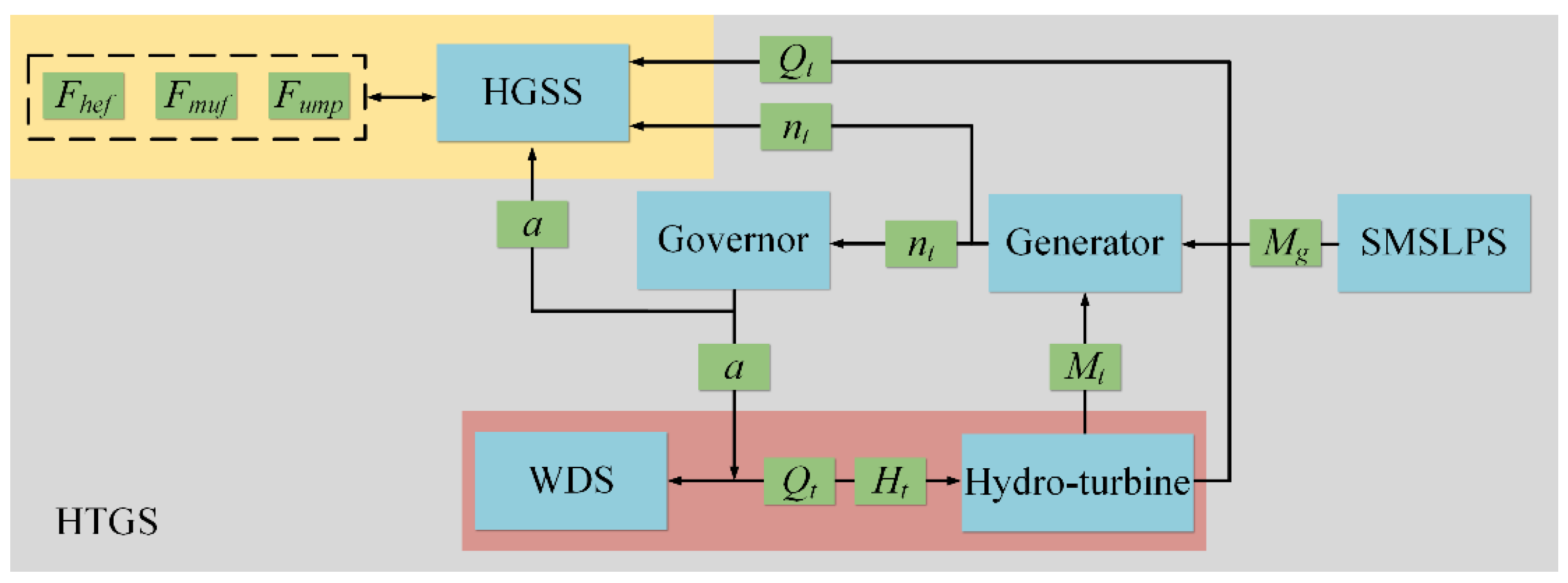
2. Transient Nonlinear Coupling Model of HGS
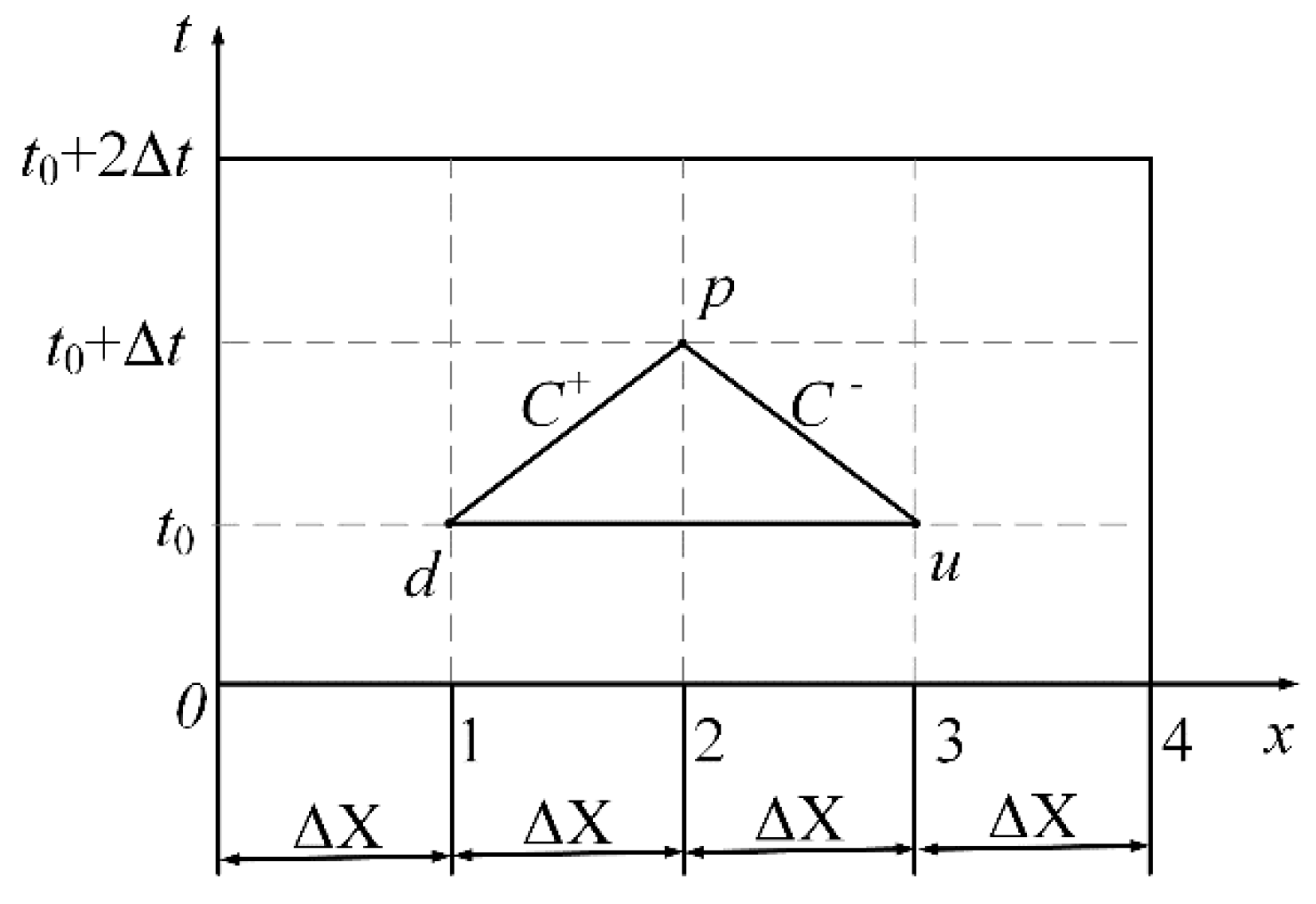
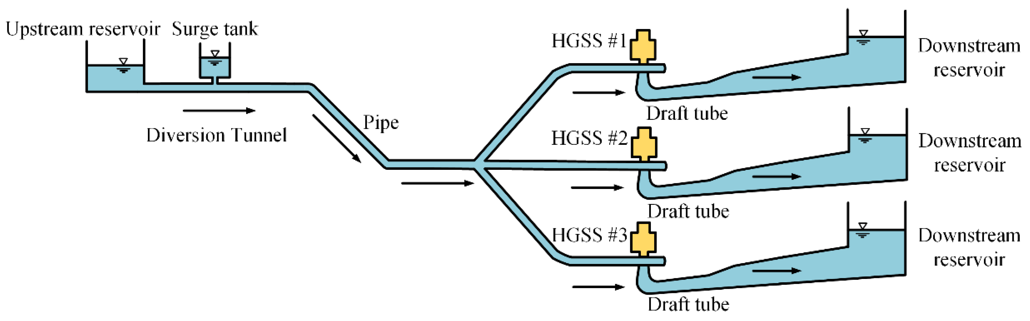
2.1. Model of WDS
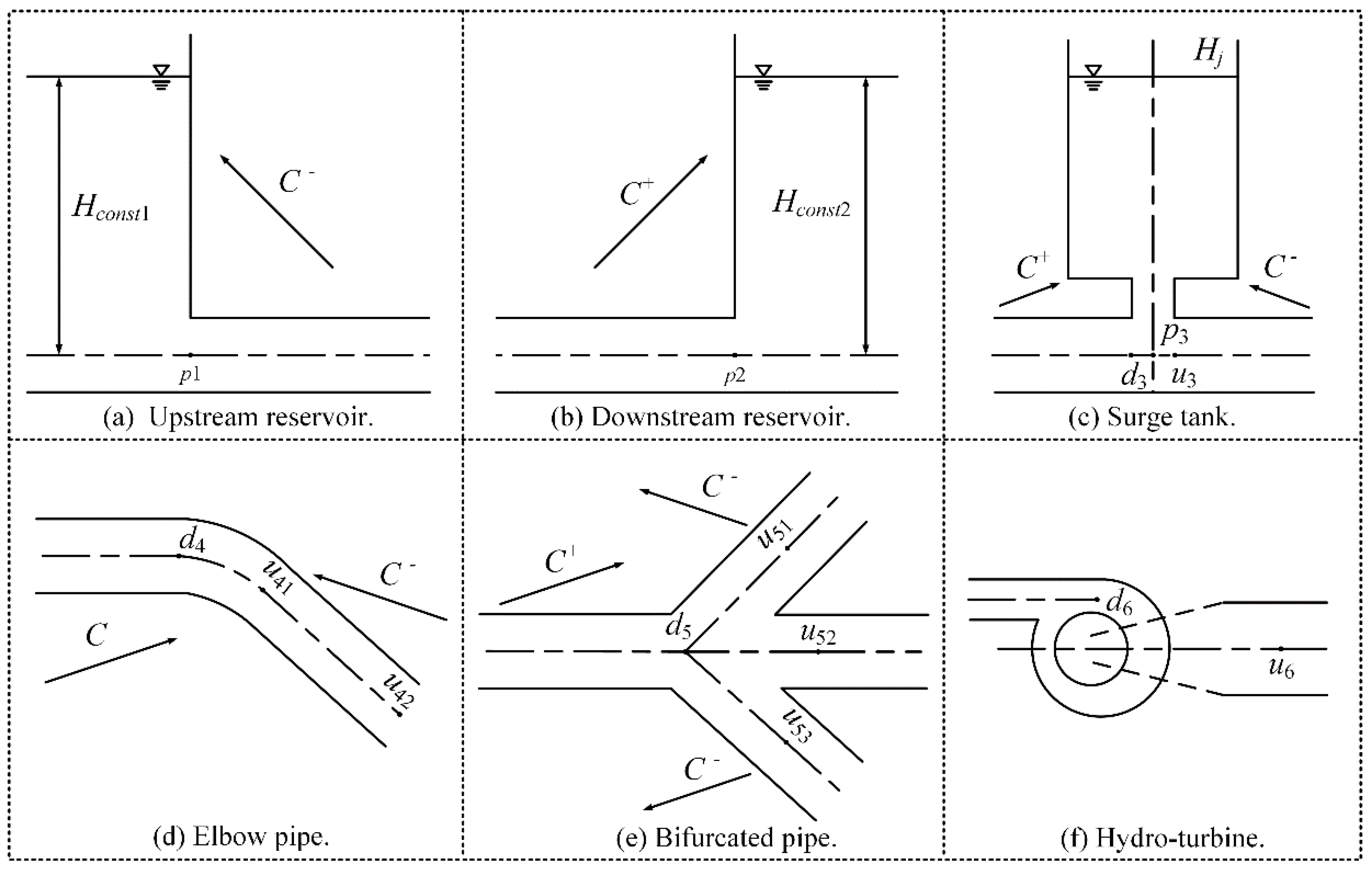
2.2. The Boundary Conditions of WDS
- (1)
- Upstream and downstream reservoirs
- (2)
- Surge tank
- (3)
- Elbow pipe and bifurcated pipe
- (4)
- Hydro-turbine
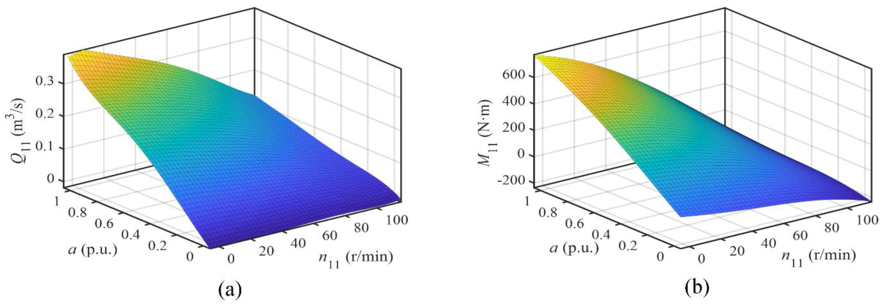
2.3. Model of Hydro-Turbine
2.4. Model of Generator and Load
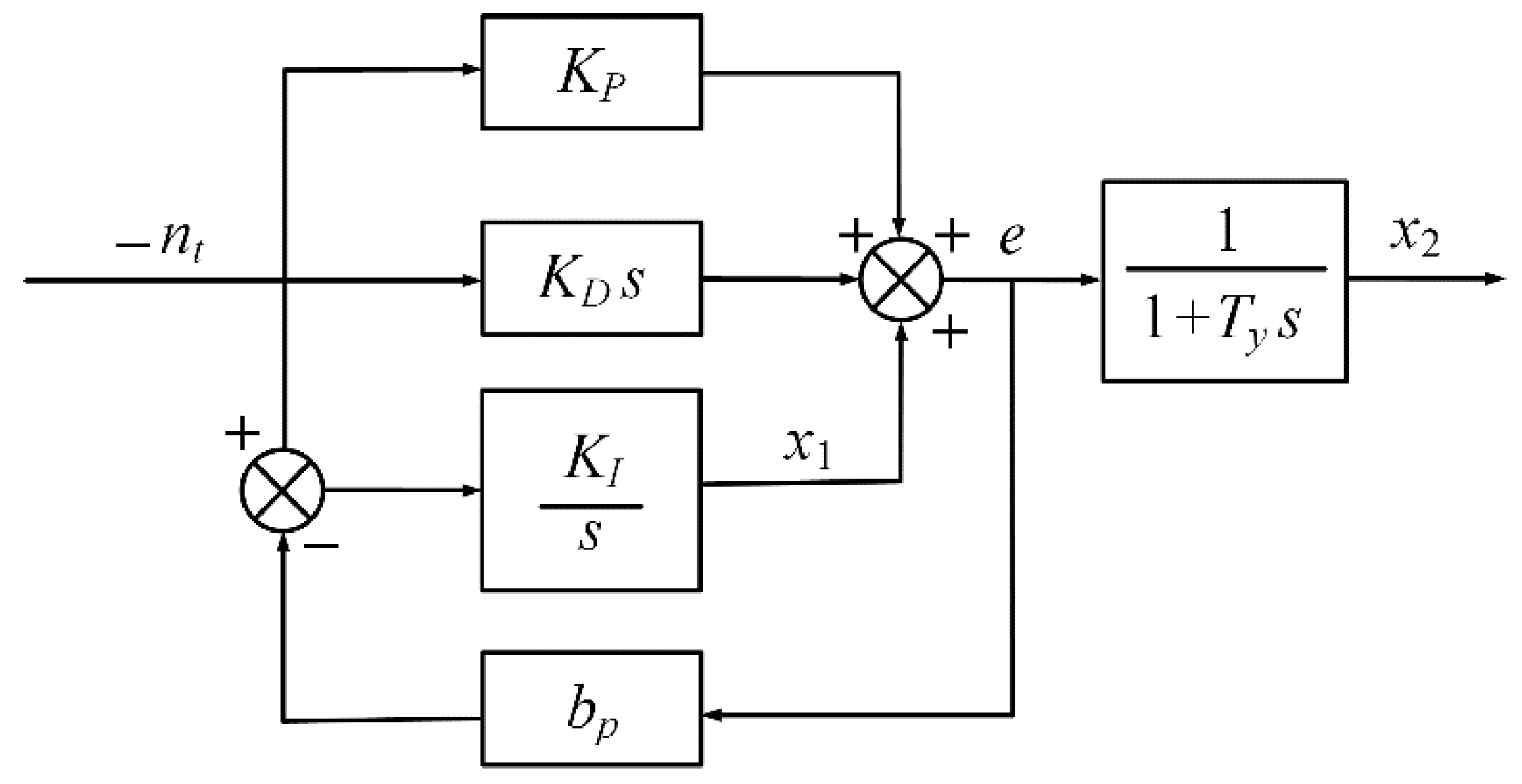
2.5. Model of PID Governor
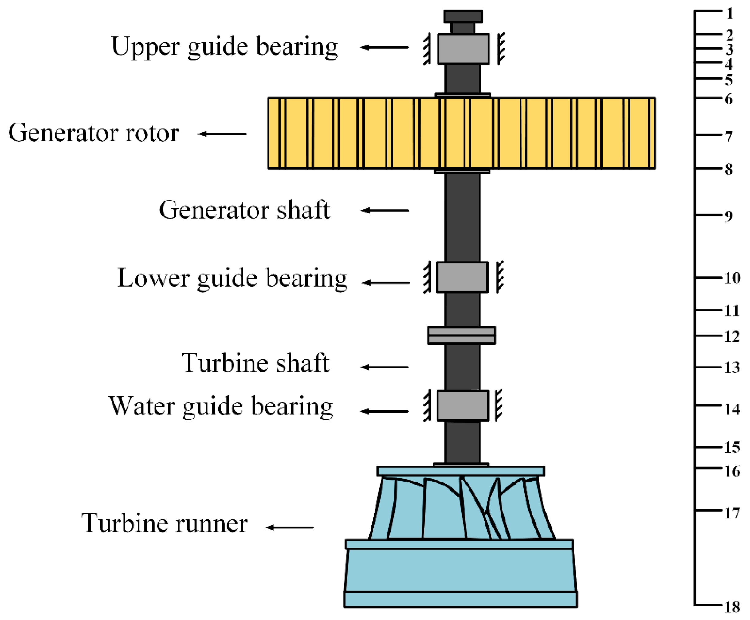
2.6. Model of HGSS
- (1)
- WNIM
- (2)
- Differential equations of motion:
- (3)
- RTMM
2.7. Additional Forces on HGSS
- (1)
- Nonlinear oil film force
- (2)
- Mechanical unbalance force
- (3)
- UMP
- (4)
- Hydraulic excitation force
2.8. Model Validation
3. Numerical Simulation and Result Analysis
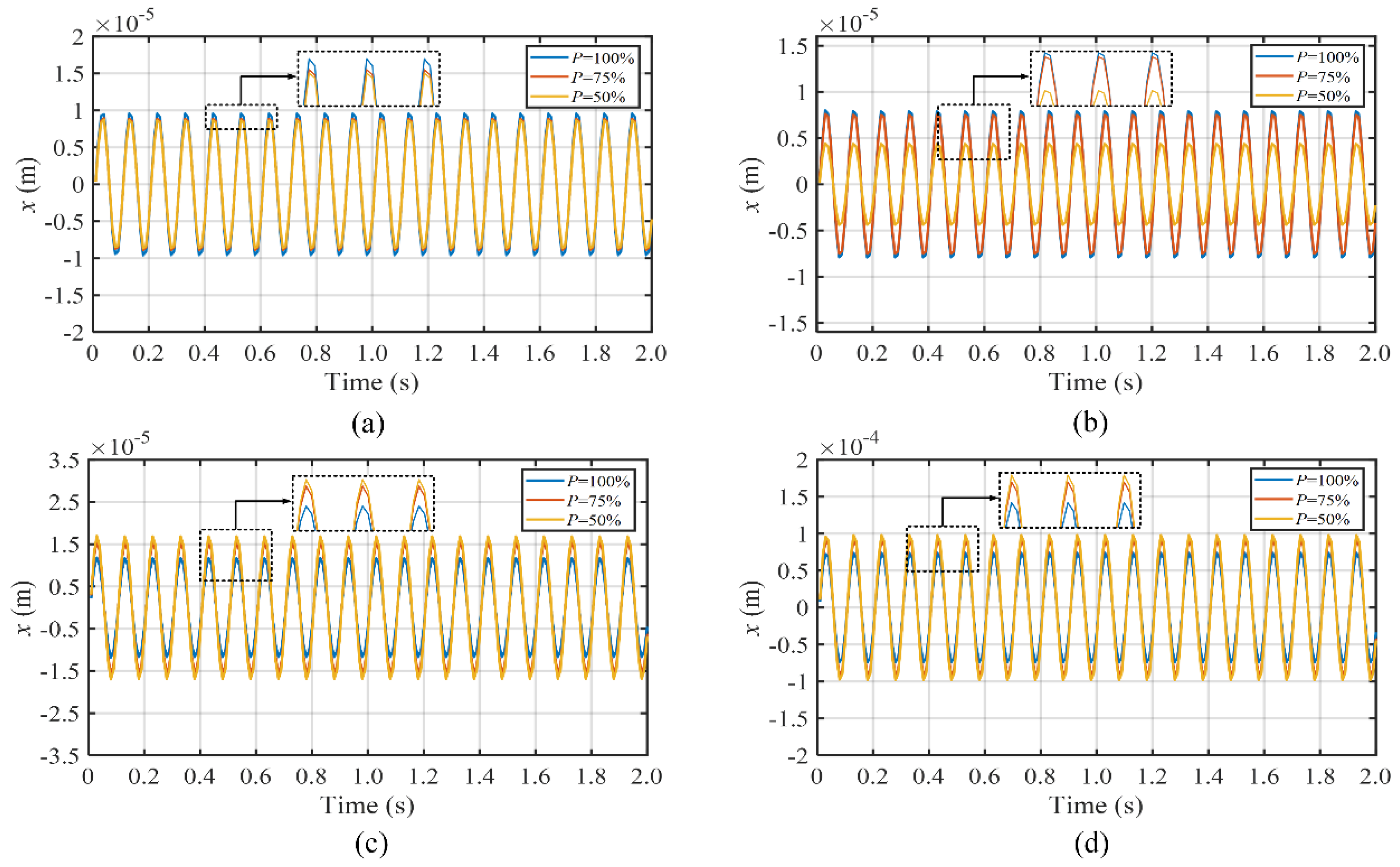
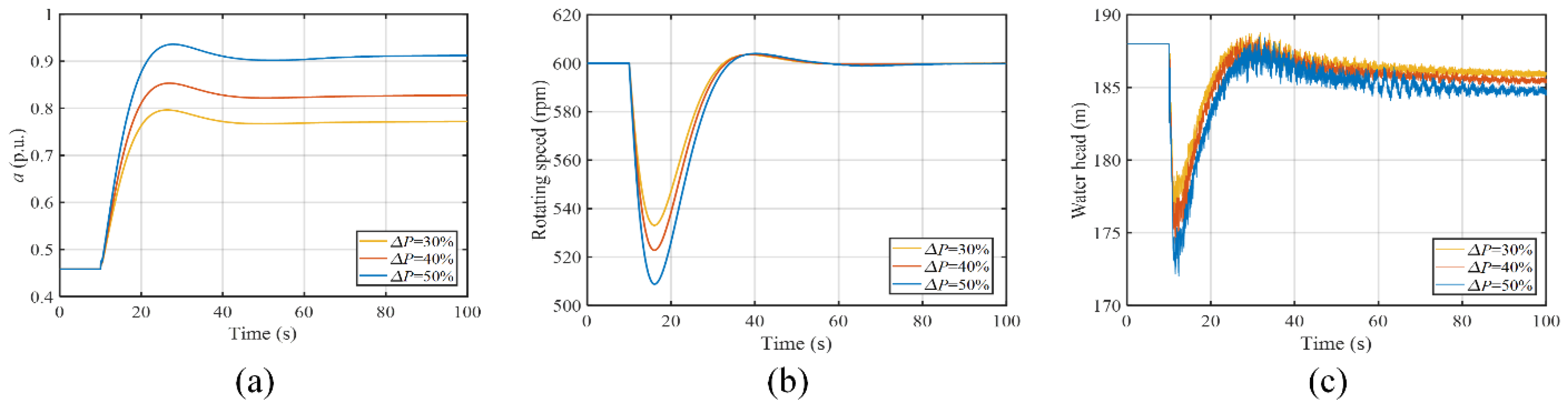
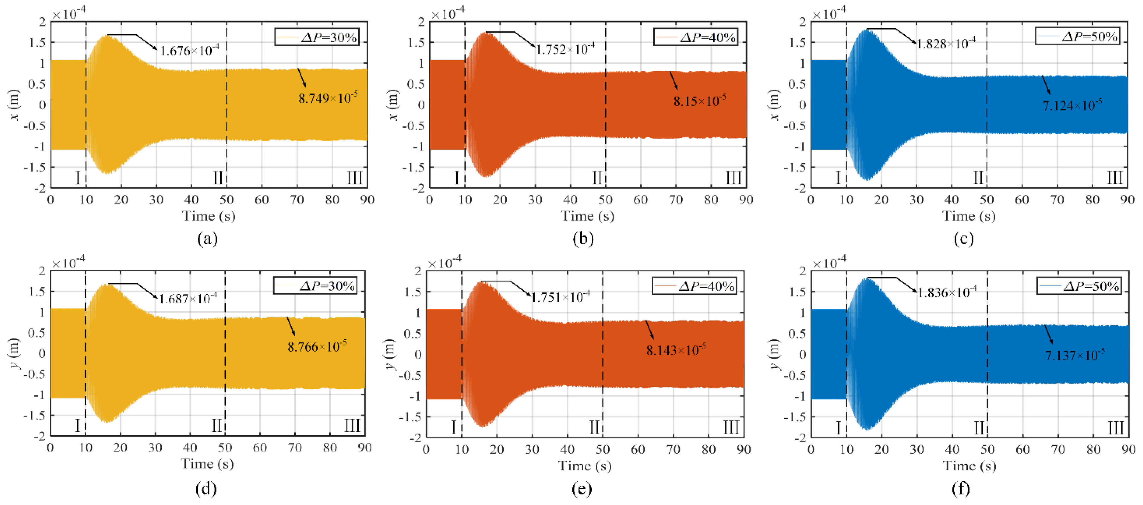
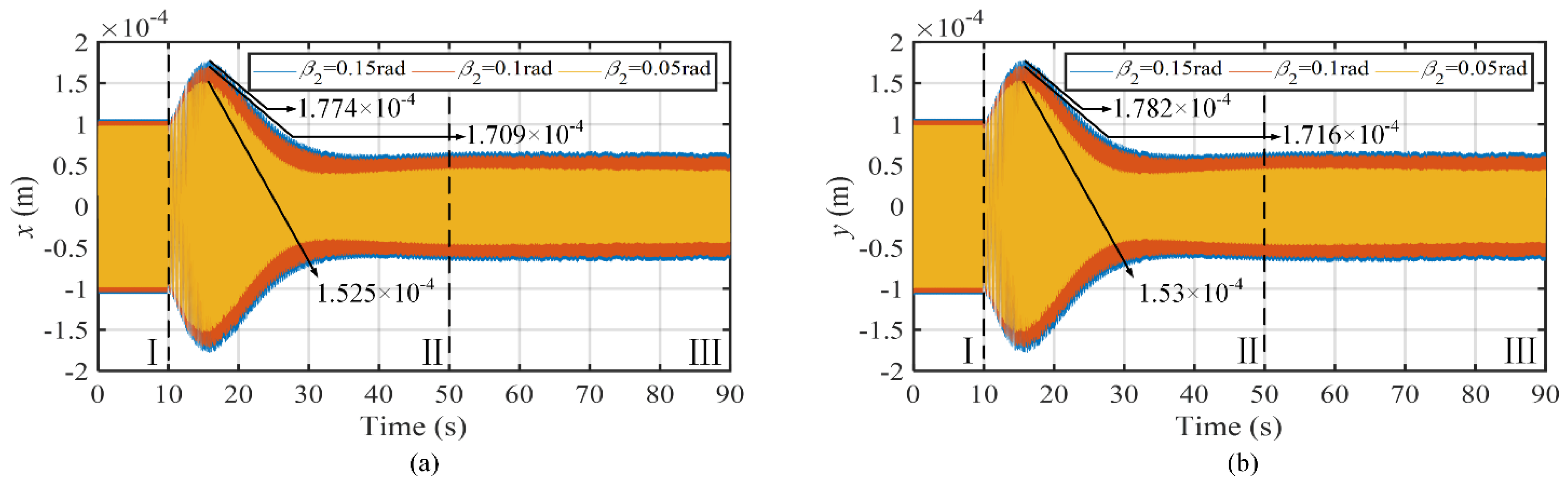
3.1. Hydraulic Factors
- (1)
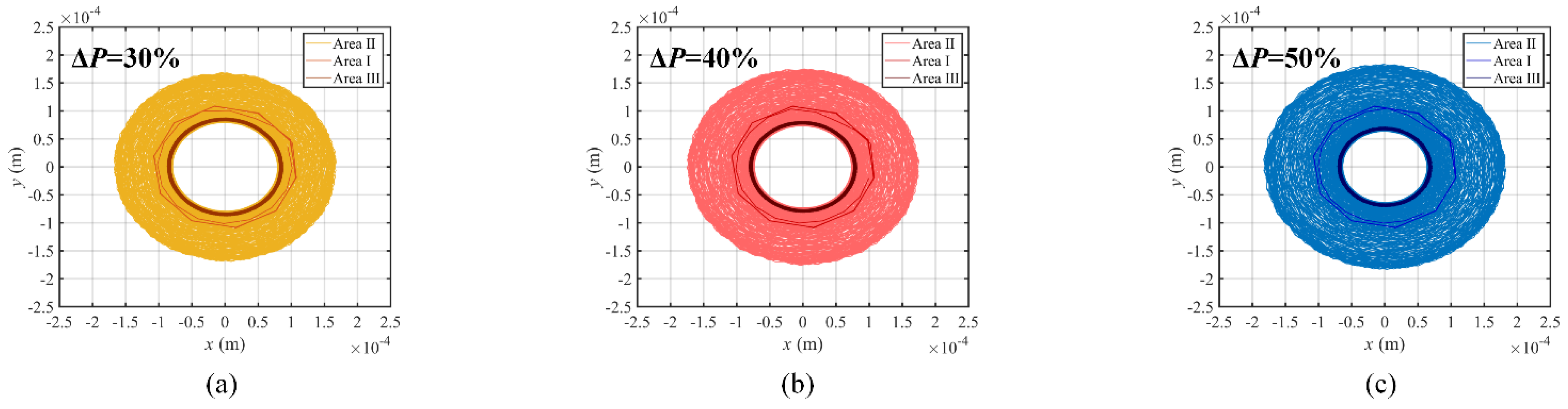
- Sudden load increasing amount
- (2)
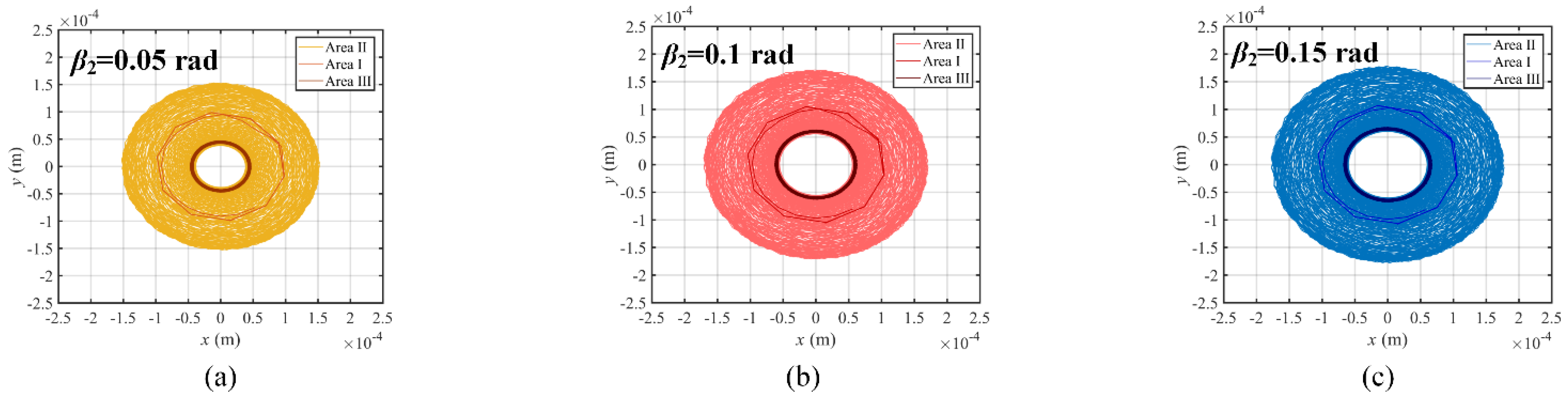
- Blade exit flow angle
3.2. Mechanical Factors
- (1)
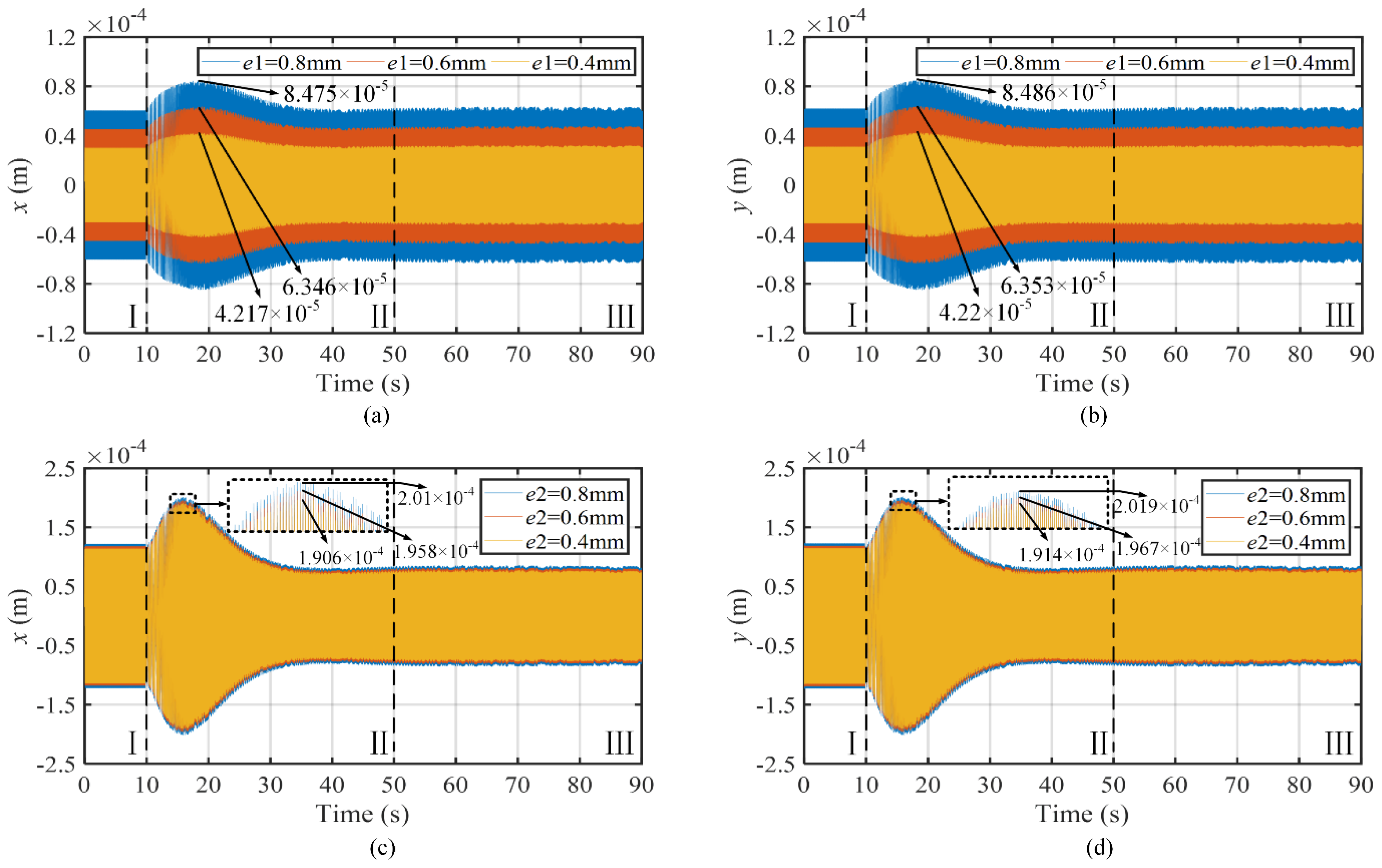
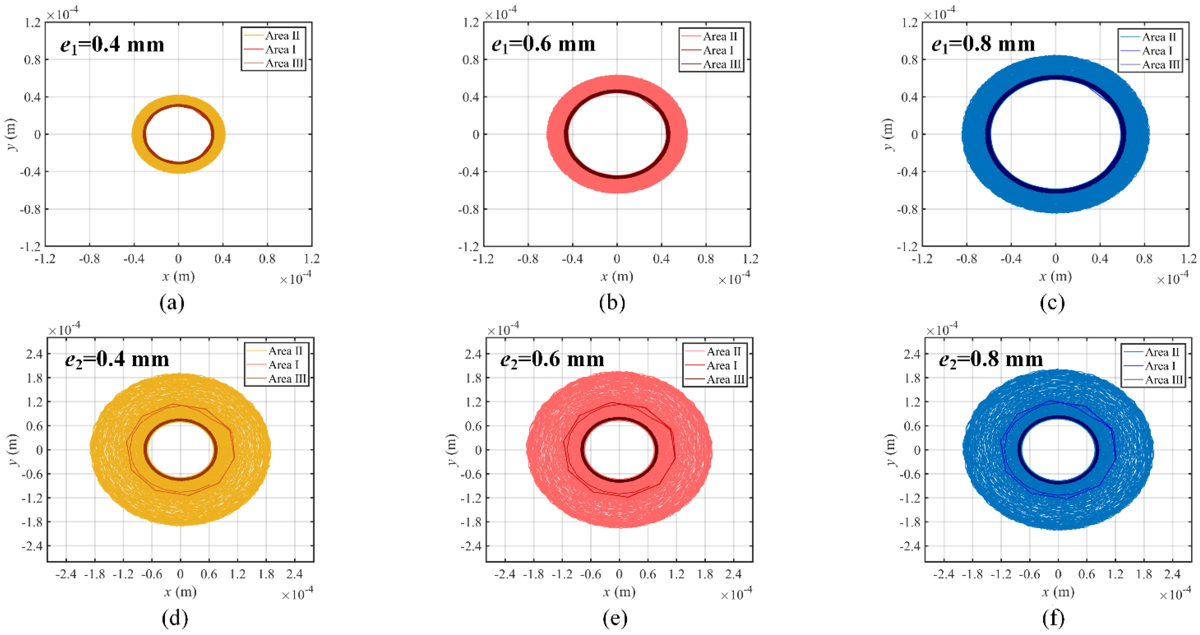
- Mass eccentricity
- (2)
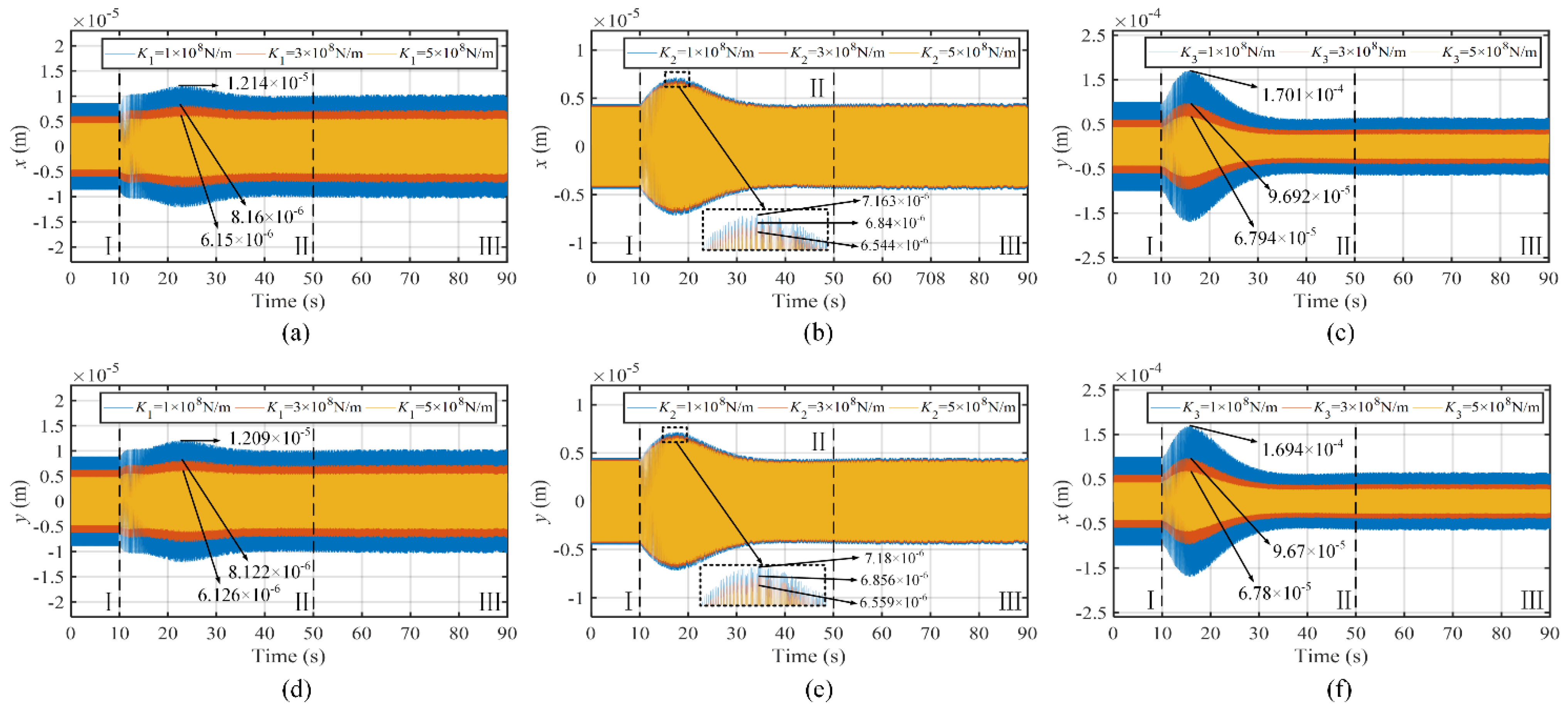
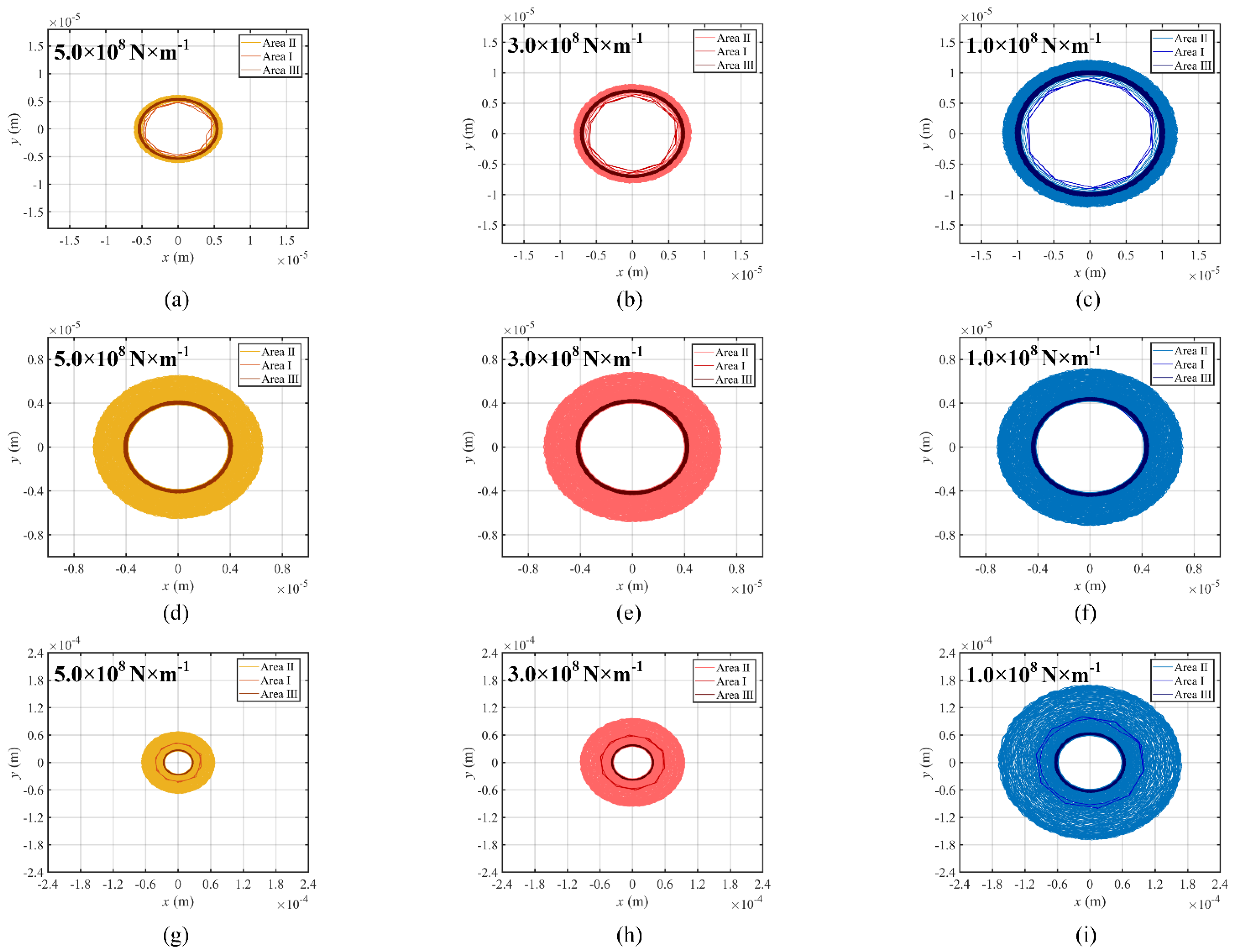
- Guide bearing stiffness
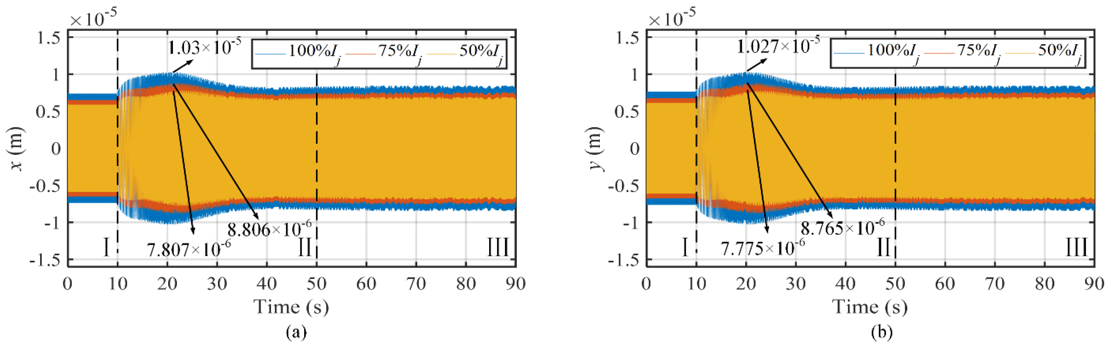
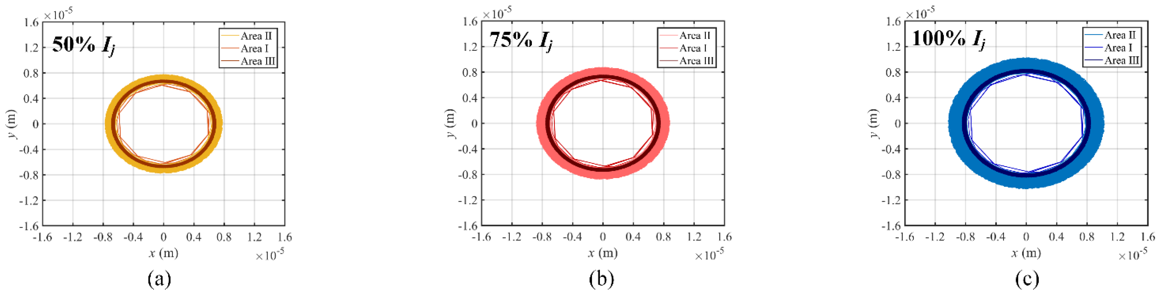
3.3. Electric Factors
- (1)
- Excitation current
- (2)
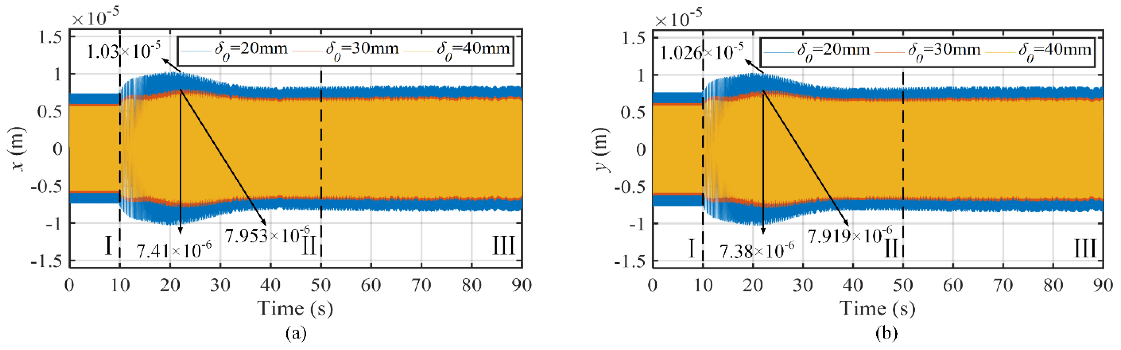
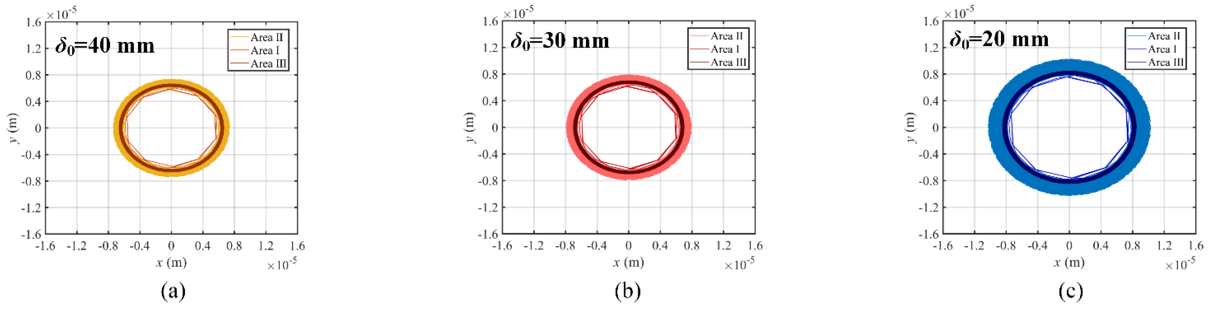
- Average air gap between stator and rotor
4. Conclusions
- (1)
- For hydraulic factors, the greater the sudden load increasing amount and blade exit flow angle, the greater the vibration of the hydro-turbine runner. The maximum vibration amplitude is increased by 69.95%, compared with that under stable operating conditions. Moreover, the vibration under a partial load is greater than that under a rated load. Hydraulic factors determine the tendency of vibration at hydro-turbine runner.
- (2)
- For mechanical factors, the vibration of HGSS increases as mass eccentricity increases and guide bearing stiffness decreases. The maximum vibration amplitude is increased by 70.46%, compared with that under stable operating conditions. The mass eccentricity has a great impact on the generator rotor, but a lesser impact on the hydro-turbine runner. The influence of the water guide bearing stiffness on the vibration response is greater than that of the upper guide bearing and the lower guide bearing.
- (3)
- For electric factors, the vibration of the generator rotor increases as the excitation current increases and the average air gap between the stator and rotor decreases. The maximum vibration amplitude is increased by 40%, compared with that under stable operating conditions.
Author Contributions
Funding
Institutional Review Board Statement
Informed Consent Statement
Conflicts of Interest
Abbreviations
| SLIP | Sudden Load Increasing Process |
| HMEPs | Hydraulic-Mechanical-Electric Parameter |
| HGSS | Hydro-turbine Generator Shafting System |
| UMP | Unbalanced Magnetic Pull |
| MOC | Method Of Characteristics |
| WNIM | Wilson-θ Numerical Integration Method |
| HGS | Hydroelectric Generating System |
| HTGS | Hydro-Turbine Governing System |
| SMSLPS | Single-Machine Single-Load Power System |
| WDS | Water Diversion System |
| RTMM | Riccati Transfer Matrix Method |
References
- Dehghani, M.; Riahi-Madvar, H.; Hooshyaripor, F.; Mosavi, A.; Shamshirband, S.; Zavadskas, E.K.; Chau, K.-W. Prediction of Hydropower Generation Using Grey Wolf Optimization Adaptive Neuro-Fuzzy Inference System. Energies 2019, 12, 289. [Google Scholar] [CrossRef] [Green Version]
- Guo, W.C. A review of the hydraulic transient and dynamic behavior of hydropower plants with sloping ceiling tailrace tunnels. Energies 2019, 12, 3220. [Google Scholar] [CrossRef] [Green Version]
- Sipahutar, R.; Bernas, S.M.; Imanuddin, M.S. Renewable energy and hydropower utilization tendency worldwide. Renew. Sustain. Energy Rev. 2013, 17, 13–15. [Google Scholar]
- Singh, V.K.; Singal, S.K. Operation of hydro power plants-a review. Renew. Sustain. Energy Rev. 2017, 69, 610–619. [Google Scholar] [CrossRef]
- Chazarra, M.; Garcia-Gonzalez, J.; Perez-Diaz, J.I.; Arteseros, M. Stochastic optimization model for the weekly scheduling of a hy-dropower system in day-ahead and secondary regulation reserve markets. Electr. Power Syst. Res. 2016, 130, 67–77. [Google Scholar] [CrossRef]
- Trivedi, C. Study of pressure pulsations in a Francis turbine designed for frequent start-stop. J. Energy Resour. Technol. 2021, 143, 1–24. [Google Scholar] [CrossRef]
- Guo, P.C.; Zhang, H.; Gou, D.M. Dynamic characteristics of a hydro-turbine governing system considering draft tube pressure pulsation. IET Renew. Power Gener. 2020, 14, 1210–1218. [Google Scholar] [CrossRef]
- Li, H.; Chen, D.; Tolo, S.; Xu, B.; Patelli, E. Hamiltonian Formulation and Analysis for Transient Dynamics of Multi-Unit Hydropower System. J. Comput. Nonlinear Dyn. 2018, 13, 101004. [Google Scholar] [CrossRef]
- Pan, Z.; Dai, Y. The influence of the overspeed protection control for the isolated grid stability. In Proceedings of the International Conference on Power System Technology, Hangzhou, China, 24–28 October 2010; pp. 1–6. [Google Scholar]
- Yan, D.L.; Wang, W.Y.; Chen, Q.J. Nonlinear modeling and dynamic analyses of the hydro-turbine governing system in the load shedding transient regime. Energies 2018, 11, 1244. [Google Scholar] [CrossRef] [Green Version]
- Liao, C.W.; Zhang, J.S. Analysis of the breast wall collapse of the surge shaft of Tianshengqiao-II hydropower station. Water Power 1994, 10, 24–26. (In Chinese) [Google Scholar]
- Ishida, Y.; Liu, J.; Inoue, T.; Suzuki, A. Vibrations of an Asymmetrical Shaft with Gravity and Nonlinear Spring Characteristics (Isolated Resonances and Internal Resonances). J. Vib. Acoust. Trans. ASME 2008, 130, 041004. [Google Scholar] [CrossRef]
- Xu, B.; Chen, D.; Behrens, P.; Ye, W.; Guo, P.; Luo, X. Modeling oscillation modal interaction in a hydroelectric generating system. Energy Convers. Manag. 2018, 174, 208–217. [Google Scholar] [CrossRef]
- Zhuang, K.; Gao, C.; Li, Z.; Yan, D.; Fu, X. Dynamic Analyses of the Hydro-Turbine Generator Shafting System Considering the Hydraulic Instability. Energies 2018, 11, 2862. [Google Scholar] [CrossRef] [Green Version]
- Favrel, A.; Junior, J.G.P.; Müller, A.; Landry, C.; Yamamoto, K.; Avellan, F. Swirl number based transposition of flow-induced mechanical stresses from reduced scale to full-size Francis turbine runners. J. Fluids Struct. 2020, 94, 102956. [Google Scholar] [CrossRef]
- Al-Hussain, K.M.; Redmond, I. Dynamic response of two rotors connected by rigid mechanical coupling with parallel misalignment. J. Sound Vib. 2002, 249, 483–498. [Google Scholar] [CrossRef]
- Yong-Wei, T.; Jian-Gang, Y. Research on vibration induced by the coupled heat and force due to rotor-to-stator rub. J. Vib. Control 2011, 17, 549–566. [Google Scholar] [CrossRef]
- Calleecharan, Y.; Aidanpaa, J.O. Dynamics of a hydropower generator subjected to unbalanced magnetic pull. Proc. Inst. Mech. Eng. Part C J. Mech. Eng. Sci. 2011, 225, 2076–2088. [Google Scholar] [CrossRef]
- Xu, Y.; Li, Z.H. Computational model for investigating the influence of unbalanced magnetic pull on the radial vibration of large hydro-turbine generators. J. Vib. Acoust. Trans. ASME 2012, 134, 051013. [Google Scholar] [CrossRef]
- Li, H.; Chen, D.; Zhang, X.; Wu, Y. Dynamic analysis and modelling of a Francis hydro-energy generation system in the load rejection transient. IET Renew. Power Gener. 2016, 10, 1140–1148. [Google Scholar] [CrossRef]
- Zeng, Y.; Zhang, L.; Guo, Y.; Qian, J.; Zhang, C. The generalized Hamiltonian model for the shafting transient analysis of the hydro turbine generating sets. Nonlinear Dyn. 2014, 76, 1921–1933. [Google Scholar] [CrossRef] [Green Version]
- Zhang, L.; Wu, Q.; Ma, Z.; Wang, X. Transient vibration analysis of unit-plant structure for hydropower station in sudden load increasing process. Mech. Syst. Signal Process. 2019, 120, 486–504. [Google Scholar] [CrossRef]
- Wu, Q.Q.; Zhang, L.K.; Ma, Z.Y. A model establishment and numerical simulation of dynamic coupled hydraulic–mechanical–electric–structural system for hydropower station. Nonlinear Dyn. 2016, 87, 459–474. [Google Scholar] [CrossRef]
- Guo, B.Q.; Xu, B.B.; Chen, D.Y.; Li, F.; Behrens, P.; Egusquiza, E. Vibration characteristics of the hydroelectric generating systems during load rejection transient process. J. Comput. Nonlinear Dyn. 2019, 14, 071006. [Google Scholar] [CrossRef]
- Rezghi, A.; Riasi, A. Sensitivity analysis of transient flow of two parallel pump-turbines operating at runaway. Renew. Energy 2016, 86, 611–622. [Google Scholar] [CrossRef]
- Chaudhry, M.H. Characteristics and finite-difference methods. Appl. Hydraul. Transients 2014, 94, 65–113. [Google Scholar]
- Riasi, A.; Tazraei, P. Numerical analysis of the hydraulic transient response in the presence of surge tanks and relief valves. Renew. Energy 2017, 107, 138–146. [Google Scholar] [CrossRef] [Green Version]
- Karlsson, M.; Aidanpää, J.-O.; Perers, R.; Leijon, M. Rotor Dynamic Analysis of an Eccentric Hydropower Generator with Damper Winding for Reactive Load. J. Appl. Mech. 2007, 74, 1178–1186. [Google Scholar] [CrossRef]
- Rezghi, A.; Riaasi, A.; Tazraei, P. Multi-objective optimization of hydraulic transient condition in a pump-turbine hydropower considering the wicket-gates closing law and the surge tank position. Renew. Energy 2020, 148, 478–491. [Google Scholar] [CrossRef]
- Yang, W.; Yang, J.; Guo, W.; Zeng, W.; Wang, C.; Saarinen, L.; Norrlund, P. A Mathematical Model and Its Application for Hydro Power Units under Different Operating Conditions. Energies 2015, 8, 10260–10275. [Google Scholar] [CrossRef]
- Guo, W.C.; Yang, J.D. Stability performance for primary frequency regulation of hydro-turbine governing system with surge tank. Appl. Math. Model. 2017, 54, 446–466. [Google Scholar] [CrossRef]
- Hou, J.; Li, C.; Tian, Z.; Xu, Y.; Lai, X.; Zhang, N.; Zheng, T.; Wu, W. Multi-Objective Optimization of Start-up Strategy for Pumped Storage Units. Energies 2018, 11, 1141. [Google Scholar] [CrossRef] [Green Version]
- Li, C.; Zhang, N.; Lai, X.; Zhou, J.; Xu, Y. Design of a fractional-order PID controller for a pumped storage unit using a gravitational search algorithm based on the Cauchy and Gaussian mutation. Inf. Sci. 2017, 396, 162–181. [Google Scholar] [CrossRef]
- Huang, S.; Chi, X.; Xu, Y.; Sun, Y. Dynamic characteristics of coupling shaft system in tufting machine based on the Riccati whole transfer matrix method. Proc. Inst. Mech. Eng. Part C J. Mech. Eng. Sci. 2016, 231, 356–371. [Google Scholar] [CrossRef]
- Yin, S.H. Vibration of a simple beam subjected to a moving sprung mass with initial velocity and constant acceleration. Int. J. Struct. Stab. Dyn. 2016, 16, 176–185. [Google Scholar] [CrossRef]
- Cui, Y.; Liu, Z.; Wang, Y.; Ye, J. Nonlinear Dynamic of a Geared Rotor System with Nonlinear Oil Film Force and Nonlinear Mesh Force. J. Vib. Acoust. 2012, 134, 041001. [Google Scholar] [CrossRef]
- Gao, H.; Song, W. Analysis on unbalance vibration and compensation for maglev flywheel. Int. J. Appl. Electromagn. Mech. 2016, 50, 177–187. [Google Scholar] [CrossRef]
- Zhang, L.; Ma, Z.; Wu, Q.; Wang, X. Vibration analysis of coupled bending-torsional rotor-bearing system for hydraulic generating set with rub-impact under electromagnetic excitation. Arch. Appl. Mech. 2016, 86, 1665–1679. [Google Scholar] [CrossRef]
- Wang, M.H. Study on Calculation of Transition Process of Long-Loaded Hydropower Station. Master’s Thesis, North China University of Water Resources and Electric Power, Zhengzhou, China, 2019. [Google Scholar]
- General Administration of Quality Supervision. Specification Installation of Hydraulic Turbine Generator Units; GB/T 8564-2003; China Standards Press: Beijing, China, 2004. (In Chinese) [Google Scholar]


| Model Parameter | Symbol | Value | Unit |
|---|---|---|---|
| Length of the tunnel | TL | 5693 | m |
| Length of the surge tank | STL | 2.3 | m |
| Length of the penstock behind the surge tank | PBSTL | 84 | m |
| Length of the sloping penstock | SPL | 58.97 | m |
| Length of the penstock behind the sloping penstock | PBSPL | 562.44 | m |
| Length of pipe 1/2/3 | PL1/PL2/PL3 | 360.6 | m |
| Diameter of the tunnel | TD | 3.2 | m |
| Diameter of the surge tank | STD | 6 | m |
| Diameter of the surge tank impedance | STID | 2.3 | m |
| Diameter of the penstock behind the surge tank | PBSTD | 3.2 | m |
| Diameter of the sloping penstock | SPD | 3 | m |
| Diameter of the penstock behind the sloping penstock | PBSPD | 3 | m |
| Diameter of pipe 1/2/3 | PD1/PD2/PD3 | 1.73 | m |
| Upstream water level | Hstart | 3456 | m |
| Downstream water level | Hend | 3252.05 | m |
| Rated output | Pr | 11 | MW |
| Rated flow rate | nr | 600 | rpm |
| Rated water head | Qr | 6.8 | m3/s |
| Runner diameter | D1 | 1.4 | m |
| Generator rotor diameter | D2 | 3.144 | m |
| Guide bearing stiffness | K | 1 × 10⁸ | N/m |
| Generator rotor mass eccentricity | e1 | 1 × 10⁻⁴ | m |
| Runner mass eccentricity | e2 | 1 × 10⁻⁴ | m |
| Uniform air gap thickness | δ0 | 2 × 10⁻² | m |
| Air permeability | μ0 | 4π × 10−7 | H/m |
| Result | Upper and Lower Water Level (m) | HGSS | The Maximum Pressure Head at the Volute (m) | The Minimum Pressure Head at the Volute (m) | The Maximum Speed Rise Rate (%) | The Maximum and Minimum Surge Level in Surge Tank (m) |
|---|---|---|---|---|---|---|
| The simulation | 3456.00 3252.05 | #1 | 252.75 | 180.01 | 58.98 | 3471.7 3453.0 |
| #2 | 252.76 | 180.03 | 58.96 | |||
| #3 | 252.74 | 180.01 | 58.95 | |||
| The experiment | 3456.00 3252.05 | #1 | 243.45 | 185.18 | 59.07 | 3476.29 3442.43 |
| #2 | 243.12 | 184.92 | 58.97 | |||
| #3 | 243.36 | 184.94 | 59.03 |
Publisher’s Note: MDPI stays neutral with regard to jurisdictional claims in published maps and institutional affiliations. |
© 2021 by the authors. Licensee MDPI, Basel, Switzerland. This article is an open access article distributed under the terms and conditions of the Creative Commons Attribution (CC BY) license (https://creativecommons.org/licenses/by/4.0/).
Share and Cite
Guo, Y.; Liang, X.; Niu, Z.; Cao, Z.; Lei, L.; Xiong, H.; Chen, D. Vibration Characteristics of a Hydroelectric Generating System with Different Hydraulic-Mechanical-Electric Parameters in a Sudden Load Increasing Process. Energies 2021, 14, 7319. https://doi.org/10.3390/en14217319
Guo Y, Liang X, Niu Z, Cao Z, Lei L, Xiong H, Chen D. Vibration Characteristics of a Hydroelectric Generating System with Different Hydraulic-Mechanical-Electric Parameters in a Sudden Load Increasing Process. Energies. 2021; 14(21):7319. https://doi.org/10.3390/en14217319
Chicago/Turabian StyleGuo, Yixuan, Xiao Liang, Ziyu Niu, Zezhou Cao, Liuwei Lei, Hualin Xiong, and Diyi Chen. 2021. "Vibration Characteristics of a Hydroelectric Generating System with Different Hydraulic-Mechanical-Electric Parameters in a Sudden Load Increasing Process" Energies 14, no. 21: 7319. https://doi.org/10.3390/en14217319
APA StyleGuo, Y., Liang, X., Niu, Z., Cao, Z., Lei, L., Xiong, H., & Chen, D. (2021). Vibration Characteristics of a Hydroelectric Generating System with Different Hydraulic-Mechanical-Electric Parameters in a Sudden Load Increasing Process. Energies, 14(21), 7319. https://doi.org/10.3390/en14217319