
Blade Dimension Optimization and Performance Analysis of the 2-D Ugrinsky Wind Turbine

Abstract
:1. Introduction
2. Numerical Methods
2.1. Regularized Lattice Boltzmann Method
2.2. Virtual Flux Method
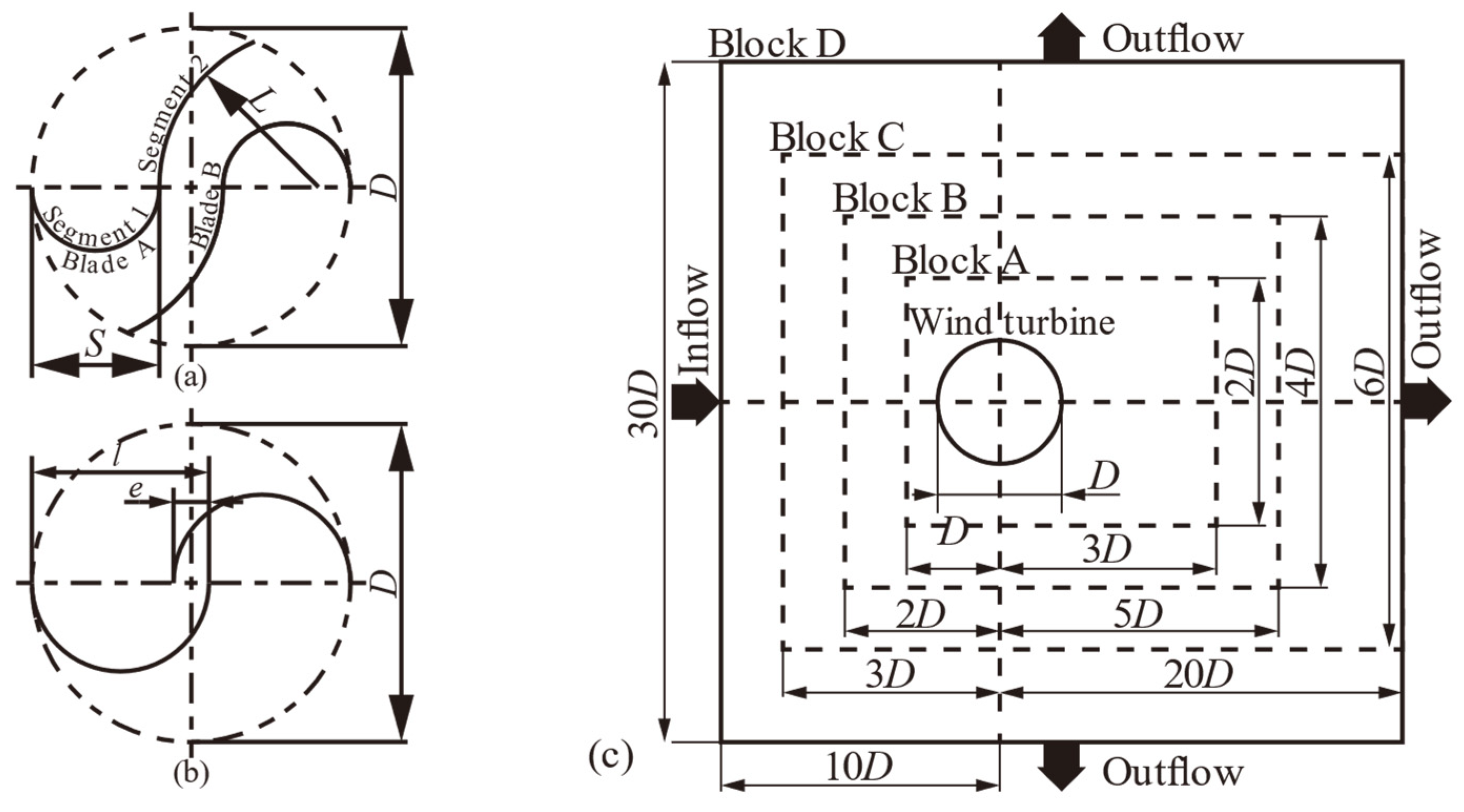
2.3. Computational Models
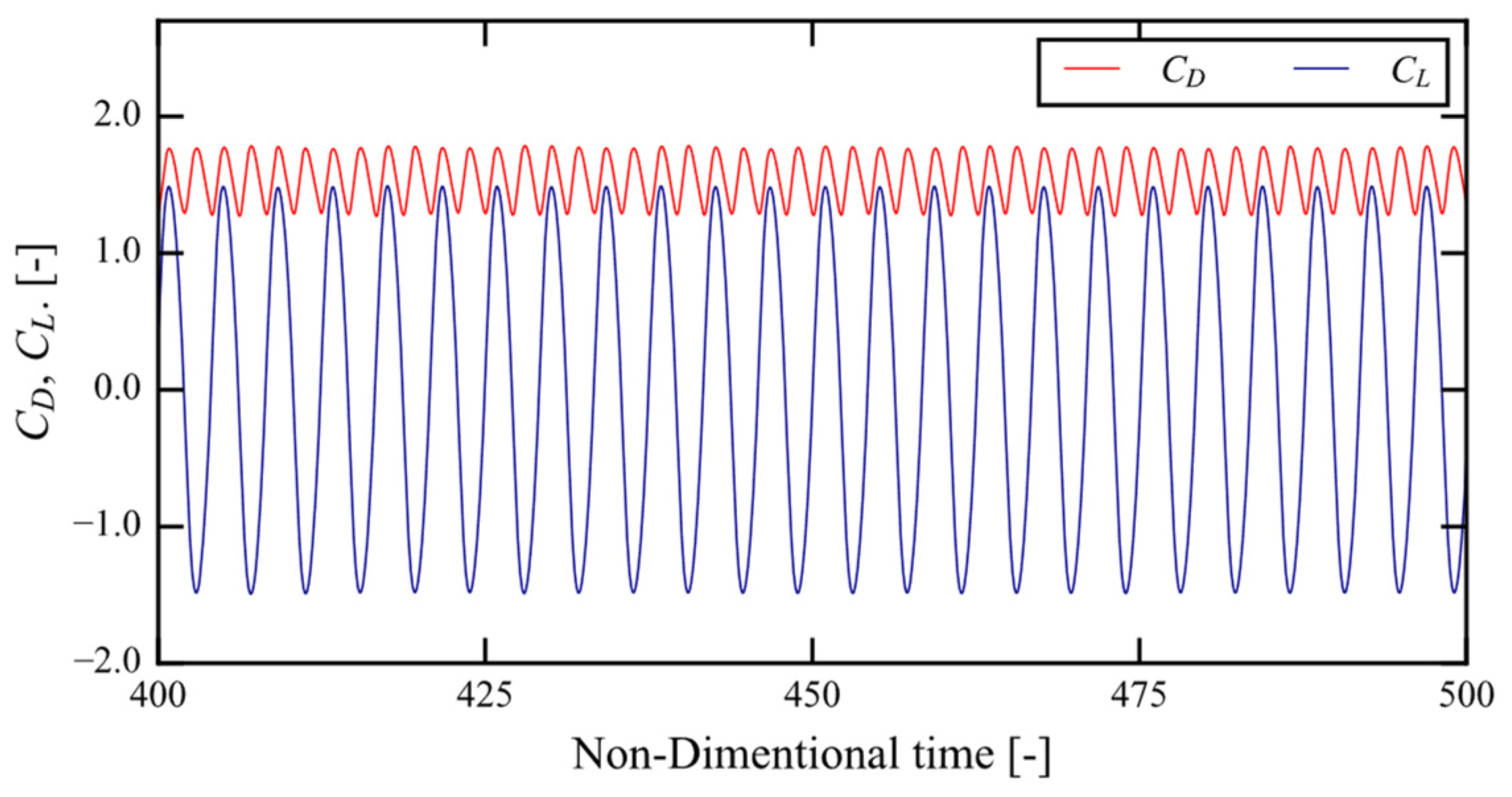
2.4. Validation
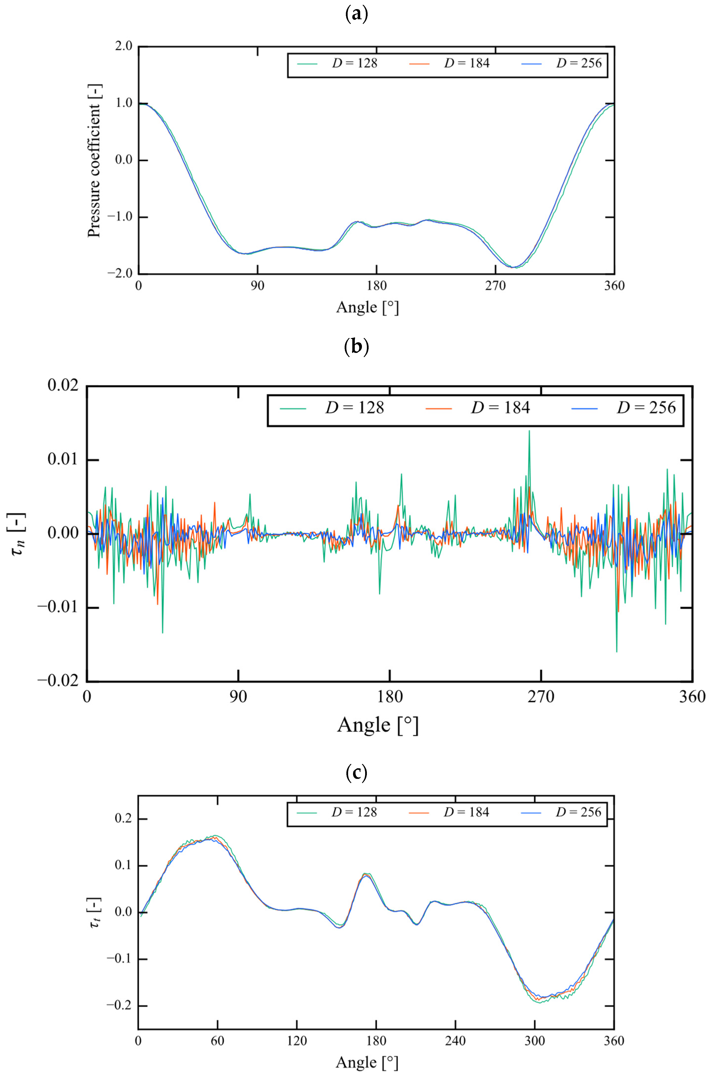
2.5. Verification
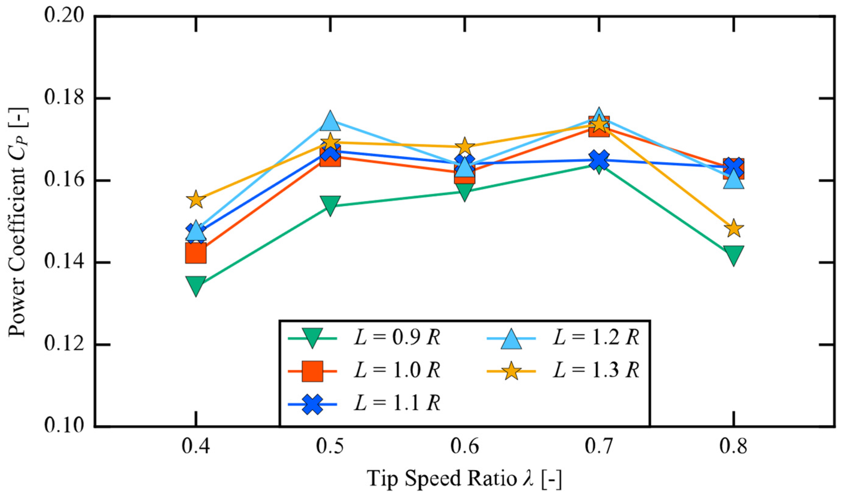
3. Results and Discussion for the Optimization of S = 0.30D and 0.40D Models
4. Conclusions
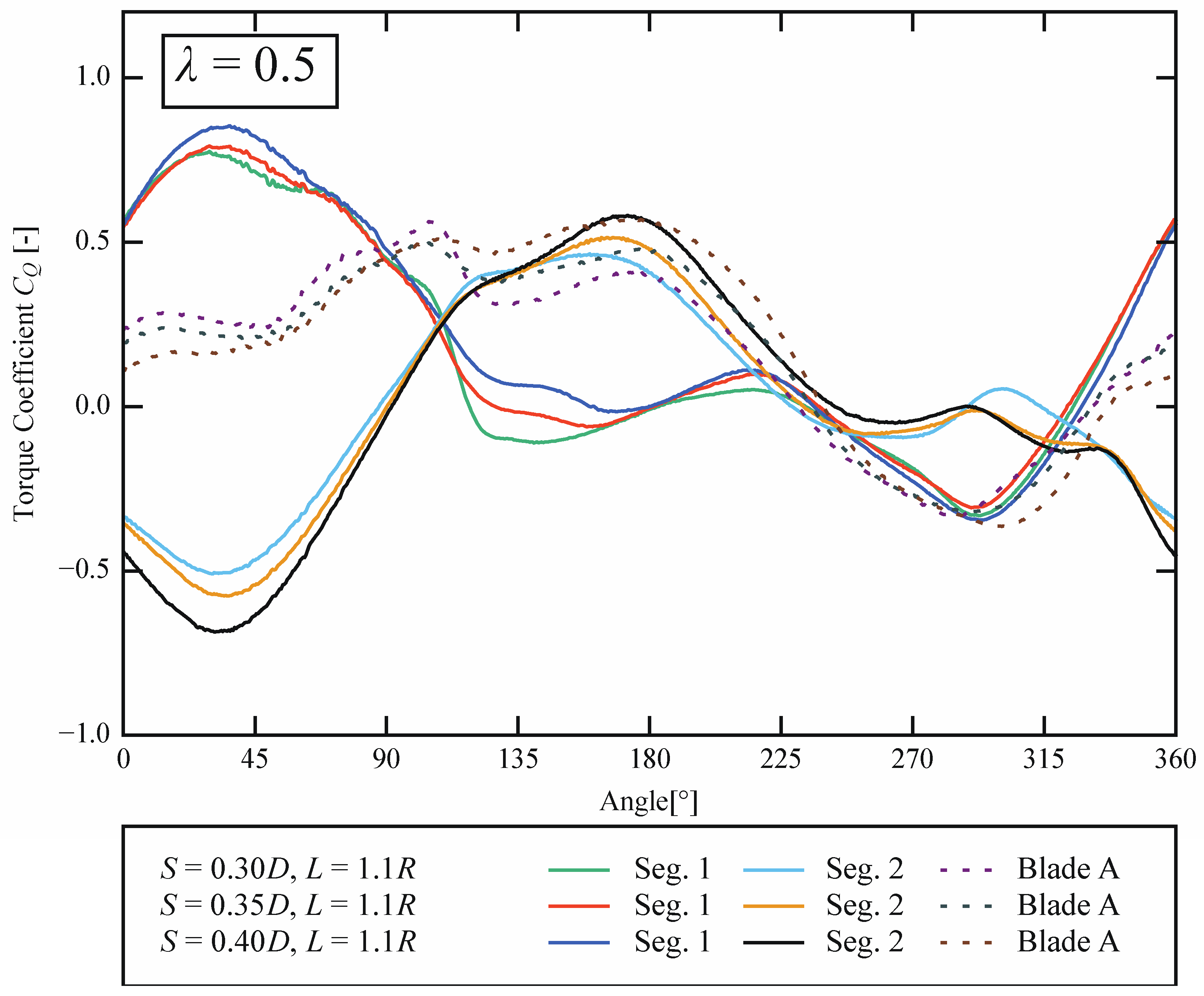
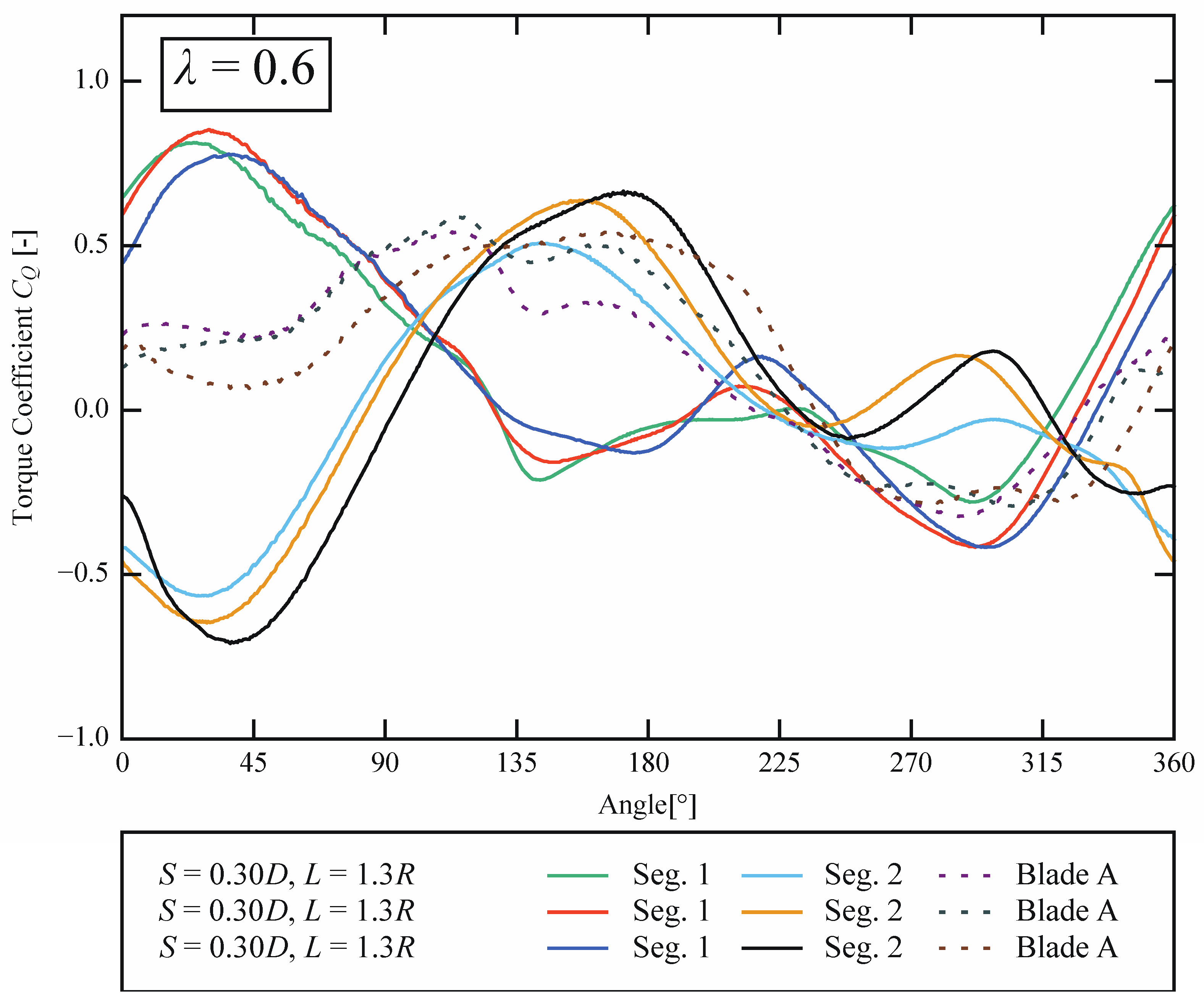
- The geometrical properties are dominant in the returning blade period of Segment 2 regardless of the TSR, and an increase in torque arm length may increase the negative torque.
- The geometrical properties are dominant in the advancing blade period of Segment 1 at λ = 0.5; however, the increase in the wind-receiving area (swept area) may not benefit at λ = 0.6.
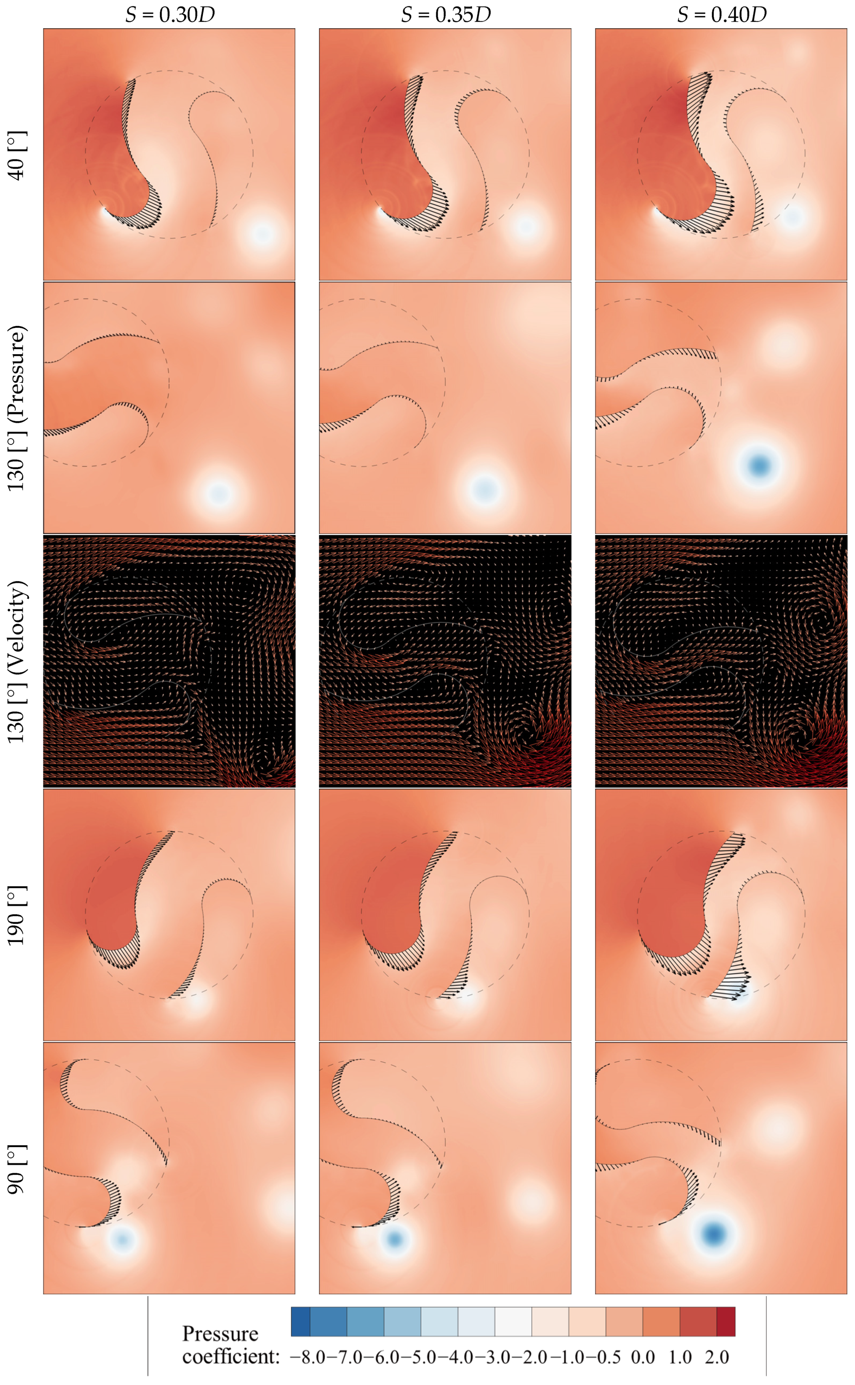
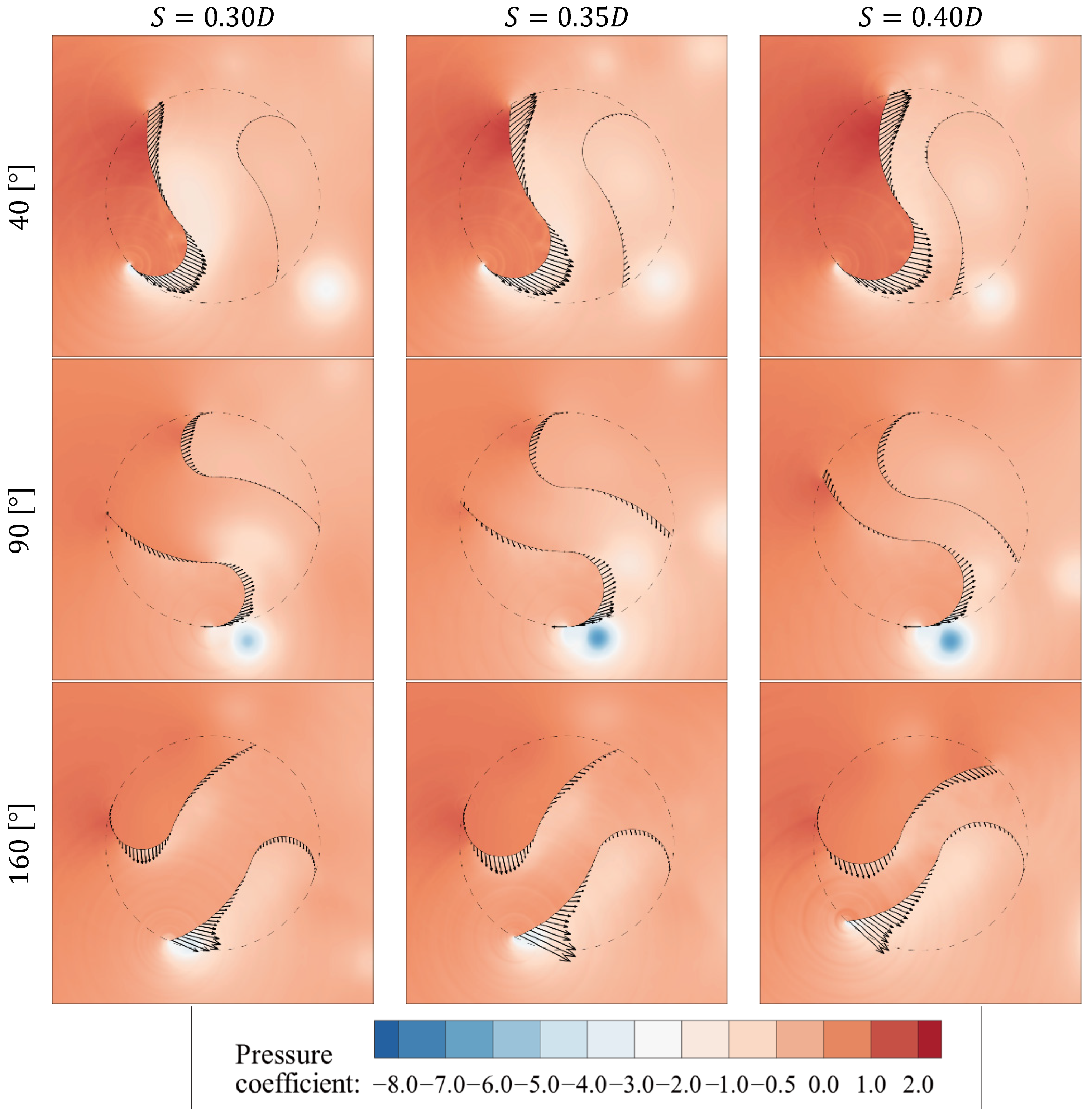
- The distance between edge vortices created on each segment may affect the growth of those vortices. This study demonstrates that a shorter distance benefits the growth of the vortex and lowers the central pressure of the vortex.
Author Contributions
Funding
Informed Consent Statement
Data Availability Statement
Conflicts of Interest
References
- Jang, H.; Kim, D.; Hwang, Y.; Paek, I.; Kim, S.; Baek, J. Analysis of Archimedes Spiral Wind Turbine Performance by Simulation and Field Test. Energies 2019, 12, 4624. [Google Scholar] [CrossRef] [Green Version]
- Roy, S.; Saha, U.K. Review on the numerical investigations into the design and development of Savonius wind rotors. Renew. Sustain. Energy Rev. 2013, 24, 73–83. [Google Scholar] [CrossRef]
- Mitchell, S.; Ogbonna, I.; Volkov, K. Improvement of Self-Starting Capabilities of Vertical Axis Wind Turbines with New Design of Turbine Blades. Sustainability 2021, 13, 3854. [Google Scholar] [CrossRef]
- Tian, W.; Song, B.; Van Zwieten, J.H.; Pyakurel, P. Computational Fluid Dynamics Prediction of a Modified Savonius Wind Turbine with Novel Blade Shapes. Energies 2015, 8, 7915–7929. [Google Scholar] [CrossRef]
- Zhang, B.; Song, B.; Mao, Z.; Tian, W.; Li, B.; Li, B. A Novel Parametric Modeling Method and Optimal Design for Savonius Wind Turbines. Energies 2017, 10, 301. [Google Scholar] [CrossRef] [Green Version]
- Alaimo, A.; Esposito, A.; Milazzo, A.; Orlando, C.; Trentacosti, F. Slotted Blades Savonius Wind Turbine Analysis by CFD. Energies 2013, 6, 6335–6351. [Google Scholar] [CrossRef]
- Chakroun, Y.; Bangga, G. Aerodynamic Characteristics of Airfoil and Vertical Axis Wind Turbine Employed with Gurney Flaps. Sustainability 2021, 13, 4284. [Google Scholar] [CrossRef]
- Müller, G.; Chavushoglu, M.; Kerri, M.; Tsuzaki, T. A resistance type vertical axis wind turbine for building integration. Renew. Energy 2017, 111, 803–814. [Google Scholar] [CrossRef] [Green Version]
- IRENA. Renewables for Refugee Settlements: Sustainable Energy Access in Humanitarian Situations; International Renewable Energy Agency: Abu Dhabi, United Arab Emirate, 2019; p. 4. [Google Scholar]
- Feng, F.; Tong, G.; Ma, Y.; Li, Y. Numerical Simulation and Wind Tunnel Investigation on Static Characteristics of VAWT Rotor Starter with Lift-Drag Combined Structure. Energies 2021, 14, 6167. [Google Scholar] [CrossRef]
- Ushiyama, I. Introduction to Wind Turbine Engineering, 2nd ed.; Morikita Publishing: Tokyo, Japan, 2013; pp. 53–60. (In Japanese) [Google Scholar]
- Ushiyama, I.; Nagai, H.; Shinoda, J. Experimentally determining the optimum design configuration for Savonius rotors. Trans. Jpn. Soc. Mech. Eng. Ser. B 1986, 52, 2973–2981. [Google Scholar] [CrossRef] [Green Version]
- Mohamed, M.; Gábor, J.; Elemér, P.; Dominique, T. Optimization of Savonius turbines using an obstacle shielding the returning blade. Renew. Energy 2010, 35, 2618–2626. [Google Scholar] [CrossRef]
- El-Askary, W.A.; Nasef, M.H.; AbdEL-hamid, A.A.; Gad, H.E. Harvesting wind energy for improving performance of Savonius rotor. J. Wind Eng. Ind. Aerodyn. 2015, 139, 8–15. [Google Scholar] [CrossRef]
- Roy, S.; Ducoin, A. Unsteady analysis on the instantaneous forces and moment arms acting on a novel Savonius-style wind turbine. Energy Convers. Manag. 2016, 121, 281–296. [Google Scholar] [CrossRef]
- Matsui, T.; Fukui, T.; Morinishi, K. Computational fluid dynamics on a newly developed Savonius rotor by adding sub-buckets for increase of the tip speed ratio to generate higher output power coefficient. J. Fluid Sci. Technol. 2020, 15, JFST0009. [Google Scholar] [CrossRef] [Green Version]
- Kazhinsky, B.B. Low-Capacity Free-Flow Hydroelectric Power Plants; Gosenergoizdat: Moscow, Russia, 1950; pp. 30–32. (In Russian) [Google Scholar]
- Sakamoto, L.; Fukui, T.; Morinishi, K. Performance Evaluation of Ugrinsky Wind Turbine using Numerical Simulation. In Proceedings of the Fluids Engineering Conference, Osaka, Japan, 6 November 2020. (In Japanese). [Google Scholar]
- Sakamoto, L.; Fukui, T.; Morinishi, K. Numerical Study on the Performance of 2-D Ugrinsky Wind Turbine Model. WIT Trans. Ecol. Environ. 2021, 254, 113–124. [Google Scholar]
- Izham, M.; Fukui, T.; Morinishi, K. Application of Regularized Lattice Boltzmann Method for Incompressible Flow Simulation at High Reynolds Number and Flow with Curved Boundary. J. Fluid Sci. Technol. 2011, 6, 812–822. [Google Scholar] [CrossRef] [Green Version]
- Tanno, I.; Morinishi, K.; Matsuno, K.; Nishida, H. Validation of Virtual Flux Method for Forced Convection Flow. JSME Int. J. Ser. B 2006, 46, 1141–1148. [Google Scholar] [CrossRef] [Green Version]
- Morinishi, K.; Fukui, T. An Eulerian approach for fluid-structure interaction problems. Comput. Fluids 2012, 65, 92–98. [Google Scholar] [CrossRef]
- Yu, D.; Mei, R.; Shyy, W. A multi-block lattice Boltzmann method for viscous fluid flows. Int. J. Numer. Methods Fluids 2002, 39, 99–120. [Google Scholar] [CrossRef]
- Chen, S.; Doolen, G.D. Lattice Boltzmann method for fluid flows. Annu. Rev. Fluid Mech. 1998, 30, 329–364. [Google Scholar] [CrossRef] [Green Version]
- Tsutahara, M.; Hiraishi, M. Study of Outflow Boundary Condition for Finite Difference Lattice Boltzmann Method. Trans. Jpn. Soc. Comput. Eng. Sci. 2006, 6, 7–12. [Google Scholar]
- Lei, C.; Cheng, L.; Kavanagh, K. A finite difference solution of the shear flow over a circular cylinder. Ocean Eng. 2000, 27, 271–290. [Google Scholar] [CrossRef]
- Matsumiya, H.; Kieda, K.; Taniguchi, N.; Kobayashi, T. Numerical Simulation of 2D Flow around a Circular Cylinder by the Third- Order Upwind Finite-Difference Method. Trans. Jpn. Soc. Mech. Eng. Ser. B 1993, 59, 2937–2943. [Google Scholar] [CrossRef] [Green Version]
- Mittal, S.; Kumar, V. Flow-induced vibrations of a light circular cylinder at reynolds numbers 103 to 104. J. Sound Vib. 2001, 245, 923–946. [Google Scholar] [CrossRef] [Green Version]
- Stinger, R.M.; Zang, J.; Hillis, A.J. Unsteady RANS computations of flow around a circular cylinder for a wide range of Reynolds numbers. Ocean Eng. 2014, 87, 1–9. [Google Scholar] [CrossRef] [Green Version]
- Fujii, K. Numerical Method for Computational Fluid Dynamics; University of Tokyo Press: Tokyo, Japan, 1994; pp. 174–180. (In Japanese) [Google Scholar]


| Data Provenance | St |
|---|---|
| Present (256 cells/D) | 0.240 |
| Lei [26] | 0.240 |
| Matsumia [27] | 0.220 |
| Mittai [28] | 0.250 |
| Stinger [29] | 0.227 |
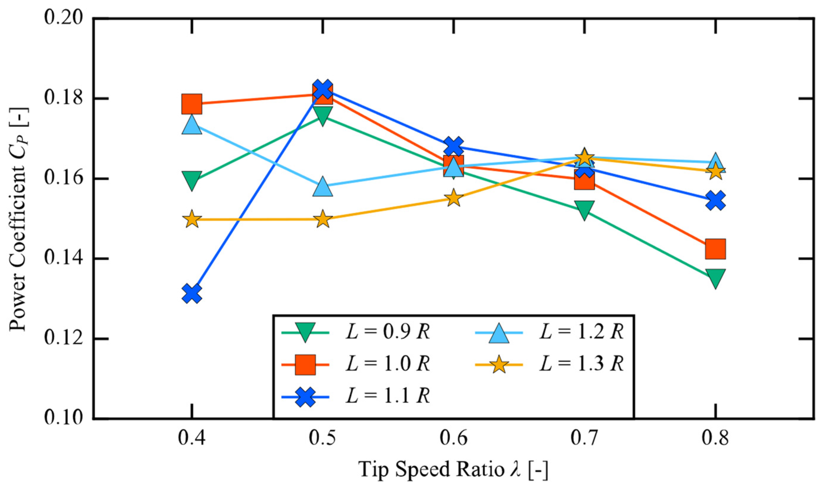
| Segment 2 | Max. CP | Ave. CP |
|---|---|---|
| 0.9L | 0.164 (λ = 0.7) | 0.158 (λ = 0.5–0.7) |
| 1.0L | 0.173 (λ = 0.7) | 0.167 (λ = 0.5–0.7) |
| 1.1L | 0.167 (λ = 0.5) | 0.165 (λ = 0.5–0.7) |
| 1.2L | 0.175 (λ = 0.7) | 0.171 (λ = 0.5–0.7) |
| 1.3L | 0.174 (λ = 0.7) | 0.170 (λ = 0.5–0.7) |
| Segment 2 | Max. CP | Ave. CP |
|---|---|---|
| 0.9L | 0.176 (λ = 0.5) | 0.166 (λ = 0.4–0.6) |
| 1.0L | 0.181 (λ = 0.5) | 0.174 (λ = 0.4–0.6) |
| 1.1L | 0.182 (λ = 0.5) | 0.171 (λ = 0.5–0.7) |
| 1.2L | 0.174 (λ = 0.4) | 0.166 (λ = 0.4–0.5) |
| 1.3L | 0.165 (λ = 0.7) | 0.161 (λ = 0.6–0.8) |
| Segment 1 | Vortex-Vortex Distance [D] |
|---|---|
| S = 0.30D | 1.02 |
| S = 0.35D | 0.86 |
| S = 0.40D | 0.76 |
Publisher’s Note: MDPI stays neutral with regard to jurisdictional claims in published maps and institutional affiliations. |
© 2022 by the authors. Licensee MDPI, Basel, Switzerland. This article is an open access article distributed under the terms and conditions of the Creative Commons Attribution (CC BY) license (https://creativecommons.org/licenses/by/4.0/).
Share and Cite
Sakamoto, L.; Fukui, T.; Morinishi, K. Blade Dimension Optimization and Performance Analysis of the 2-D Ugrinsky Wind Turbine. Energies 2022, 15, 2478. https://doi.org/10.3390/en15072478
Sakamoto L, Fukui T, Morinishi K. Blade Dimension Optimization and Performance Analysis of the 2-D Ugrinsky Wind Turbine. Energies. 2022; 15(7):2478. https://doi.org/10.3390/en15072478
Chicago/Turabian StyleSakamoto, Luke, Tomohiro Fukui, and Koji Morinishi. 2022. "Blade Dimension Optimization and Performance Analysis of the 2-D Ugrinsky Wind Turbine" Energies 15, no. 7: 2478. https://doi.org/10.3390/en15072478
APA StyleSakamoto, L., Fukui, T., & Morinishi, K. (2022). Blade Dimension Optimization and Performance Analysis of the 2-D Ugrinsky Wind Turbine. Energies, 15(7), 2478. https://doi.org/10.3390/en15072478