Abstract
In this paper, the problem of modeling memristors is studied. Two types of memristors with carbon and tungsten doping fabricated by the Knowm Inc. are tested. The memristors have been examined with either sinusoidal or triangle voltage wave periodic excitation. Some different frequencies, amplitudes and signal shapes have been applied. The collected data have been averaged and subjected to high frequency filtering. The quality of measurement data has also been discussed. The averaged measurement has been modeled using three popular memristor models: Strukov, Biolek and VTEAM. Some additional feathers to the considered models have been proposed and tested. Memristor is usually modeled by a set of algebraic-differential equations which link both electrical values (i.e., voltage and current) and the internal variable(s) responsible for the element dynamics. The interior-point with box constrains optimization method has been used to obtain the optimal parameters of the memristor model that fit best to the collected data. The results of the optimization process have been discussed and compared. The sensitivity to the different frequency range has been also examined and reviewed. Some conclusions and future work ideas have been postulated.
Keywords:
SDC memristor; memristor modeling; measurements; Strukov model; Biolek window; VTEAM model 1. Introduction
Memristor devices are an emerging topic that have attracted many researchers to study the possibility of using them in applications including in-memory computations, neuromorphic computing and also as non-volatile memory elements. This attraction has boosted up right after the discovery of the real memristors in May 2008 by a team of scientists from HP Labs, under the leadership of R. Stanley Williams [1]. It is claimed that memristors can be used for building efficient memory structures with larger capacity and improved performance [2]. It is shown that memristor based memories may have densities two orders of magnitude larger than RAM memories. The in-memory computation concept is very interesting considering the problem well known as the von Neumann bottleneck, i.e., the restrictive limit of data bandwidth between the CPU and RAM [3]. Memristors are also considered as a good candidate for analog filters tuned by changing the resistance of the memristors [4], switches, registers, and many more. Furthermore, networks of memristor based oscillators may achieve the processing power of biological systems due to their high connectivity and capabilities of carrying out parallel computations [5]. The bio-inspired or even brain-inspired computation concept seems to be very attractive for the solution of many complex tasks with higher efficiency then contemporary computer systems [6,7].
Memristor is a two-terminal passive element that has the ability to retain its state. In general, the state is expressed by its resistance, which depends on the history of the magnetic flux or the electric charge of the element. This concept has been introduced by L. O. Chua in their famous paper published in the year 1971 [8]. In other words, when the power supply is switched off, the element retains the state (no charge or no flux in the element). This element is the complement to four known elements R, L and C. Chua has defined a number of properties expressing the element to be considered as a memristor, known as the memristor fingerprints [9]. One of the properties is that under any bipolar periodic stimulation one gets a particular hysteresis loop that passes through the origin on the plane. This property expresses the element to be passive (dissipative) and explains its resistance variation. The frequency of the bipolar stimulus changes the loop’s shape. Its area decreases monotonically when f grows [10]. In theory when the frequency of the excitation signal goes to infinity the loop becomes a curve passing through zero. The real memristors exhibit this phenomena already for very large frequencies.
The HP lab proposed the sandwiched structure of metal-insulator-metal (MIM). The basic idea is that when a strong electric field is applied to the element, a conductive filament is formed in a dielectric layer, which under small electric fields works as an insulator. The oxide film is less than 5 nm thick and contains two layers. First insulating and second with the high conductivity property oxygen-poor . Then under the voltage that in such small dimensions creates the high electric field in the active layer. The excited electric field is sufficient that oxygen vacancies start to drift, shifting the dividing line between and . The ions drift forms conductive filaments in the oxide film. This shift of the dividing line has a strong impact on the structure conductivity. The geometrical limitation creates two border lines of the possible memristor state. Therefore, one can distinguish two physical states: the low resistance state (LRS) and the high resistance state (HRS). Several memristor elements based on various materials have been proposed after the fabrication of the HP memristor: semiconductor spintronics devices [11], amorphous silicon based devices [12] and memristors in ferroelectric tunnel barriers [13].
In this paper, the investigated elements are the self-directed channel (SDC) memristors [14]. These elements are ion-conducting devices. The active layer of the device is made of chalcogenide material GeSe/SnSe/Ag. Unlike the previously described metal–ion devices where the electric field creates conducting filaments between metal electrodes, the SDC device constrains the Ag ions movement into the chemically created channels. Permanent conductive channels in the SDC device are generated by inducing an electric field which causes the metal-catalyzed reaction. The device conductivity is determined by the amount of Ag within the channel [15]. The SDC memristor has the active layer doped to enhance and optimize the memristor properties. In this work, we consider the SDC memristors with two kinds of doping agents, i.e., tungsten or carbon. These devices have been purchased from Knowm Inc. Memristors are packaged in an encapsulated edge board with 16 elements and provided with a breakout board, which makes the measurements simpler and more reliable. In general, the behavior of the devices of a given kind is similar, but to keep the consistency of the acquired data, the authors selected the memristor element and all measurements were performed over the same two elements with the given doping agent.
2. Memristors Models
Two existing memristor models are considered in this work: the Strukov model [1] and the VTEAM model [16]. Two window functions are considered for the Strukov model: the rectangular window and the Biolek window [17]. Some improvements of the model have been proposed. It is important to add that the selected models are simple and have a compact structure, which is attractive when the nonlinear optimization algorithms are involved.
2.1. Strukov Model
In the Strukov model, also referred to as the linear ion drift model, it is assumed that the velocity of the ions drift is linearly proportional to the electric field. For this model, the relation between the current i and the voltage v is given by
where represents the relative width of the low-resistance region. It also takes a role of the state variable of the element. The minimal and maximal element resistances are described by and accordingly. They represent the low and high resistance element states. The relative width changes with the current according to the formula:
The relative width is the continued function on the interval . The requirement that is fulfilled by multiplying the RHS of the above equation by the rectangular window function
In Equation (2), the constant k depends on the properties of the material used and the geometry of the memristor element. The Strukov model depends on three real-valued parameters, i.e., , and k.
2.2. Biolek Window Function
Proposed in the previous section, the rectangular window function does not characterize certain physical phenomena in the memristor structure. It is noticed that the dynamics of the model described in Section 2.1 slows down when x is close to zero or one. One of the possible amendments is to update the window function (3). In the literature, several different window functions have been urged [17,18,19]. Here, the Biolek window function [17] is used.
, denotes for the sign function, and p is a positive integer. The Biolek window function defined by Equation (4) is modified by introducing the absolute value instead of parentheses around the factor [20]. This allows us to consider all integers p instead of only even numbers as in the original.
2.3. Asymmetric Strukov Model
Fabricated memristor nano-devices cannot be considered as symmetric because different switching phenomena are observed under different polarities of applied voltage or the current direction. This forces us to modify the model (2) described in Section 2.1. One of the possible options of model modification is to use different model parameters for different polarities of the input signal. Then the dynamic part of the modified Strukov model can be presented as:
The parameters and define the memristor dynamics for positive and negative polarity of the current i. Additionally, the modified Strukov model is presented with two different window functions and which also depend on the current direction. In the case of Biolek window, it means that window functions have two additional different p parameters and .
Six parameters define the asymmetric Strukov model with Biolek windows: , , , , and . Four of them are real-valued and two are integer-valued numbers.
2.4. Vteam Model
In the intensive measurement of the real memristors, it has been noticed that there exists a certain current (voltage) threshold below which the device does not change its state variable, i.e., the memristor dynamic disappears. In other words, in order to change the resistance of the memristor, one has to apply the input signal exceeding a certain threshold. The Voltage ThrEshold Adaptive Memristor (VTEAM) model is based on that phenomenon [16]. In this work, author uses the modified VTEAM model proposed in [20]. The internal state variable w is confined to the interval . Then the VTEAM model is defined by:
If the voltage v belongs to the interval of , then w does not change the threshold phenomenon. Six parameters of the VTEAM model are real-valued (, , , , , ) while two of them are integer-valued ( and ). Note that the variable has only a scaling effect on the local resistance, so it can be fixed to a certain value, thus it does not need to be considered in the optimization process. In this work, the authors set .
3. Experimental
In this section, the memristor measurement setup will be explained. Moreover, the measurement results are discussed and compared.
3.1. Measurement Setup
The devices under study were SDC memristors with two kinds of doping agents, i.e., tungsten and carbon. In order to measure the characteristics of the memristor device it is connected in series with the linear resistor . Its main role is to protect the memristor device from burning out by limiting the current. Some manufacturer recommendations for the current limits of the tested devices were applied. Two different series resistors were used. In the case of tungsten dopant, it was which limits the current with the applied voltages amplitudes below , and for memristors with carbon dopant the series resistor was as the recommended current needs to be lower then 50 A. The voltage measured over the series resistor is proportional to the current, so this measurement permits obtaining the relation of the element.
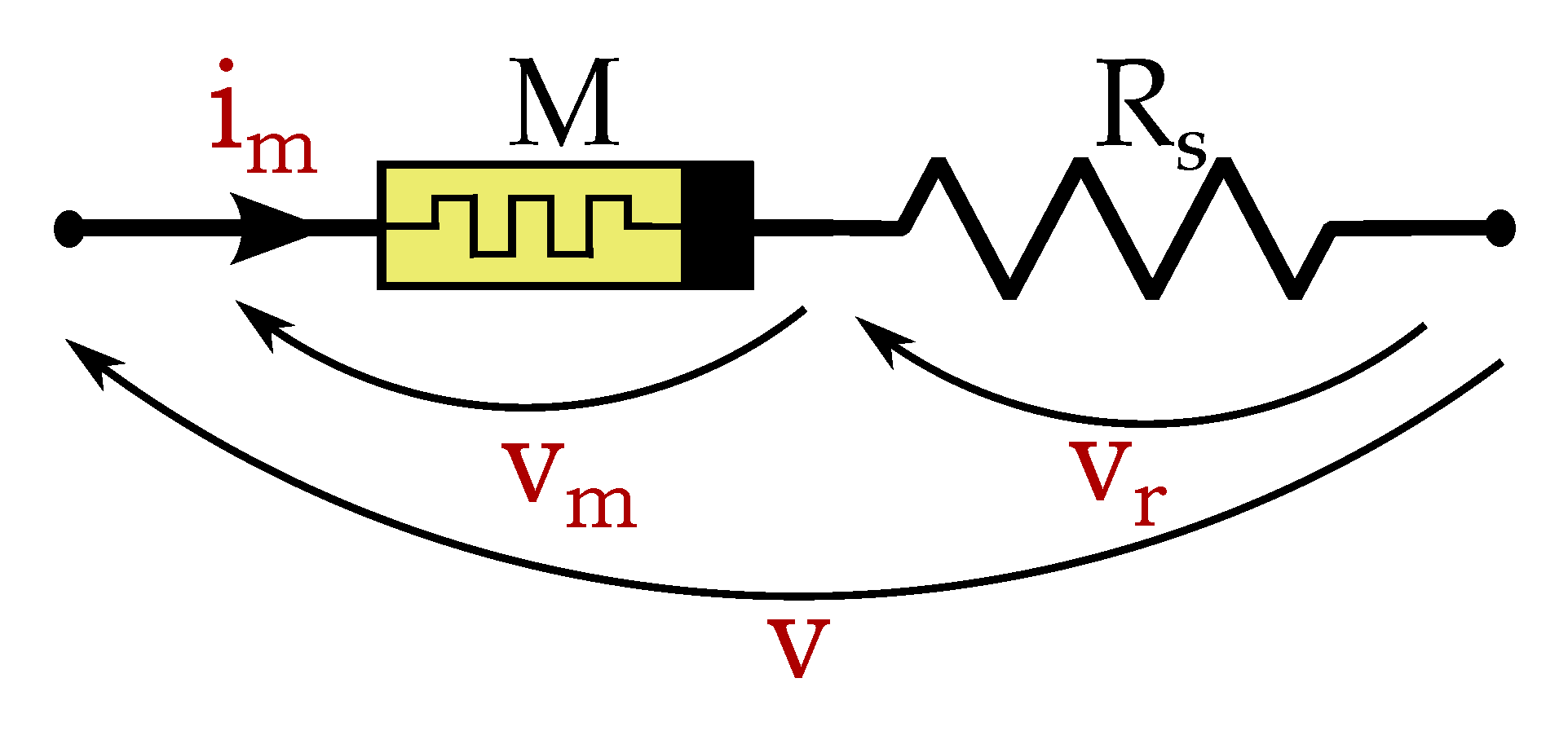
The setup of the measurement connection with the provided voltage indications used in this work has been presented in Figure 1. Signal has been generated by the signal generator device RIGOL DG1020. The response signals and were acquired using a myDAQ oscilloscope manufactured by National Instruments. All acquisition setup was carried out with the LabVIEW software environment.

Figure 1.
Measurement circuit.
Before testing procedures, the memristor needs to be formed. Forming entails applying a gradually increasing voltage until the necessary conductive pathways are formed. After the forming procedure, the measurement circuit is excited by the periodic signal . In this work, the memristor was tested by the sinusoidal voltage wave signal and the triangle wave signal that can be expressed as . Three different amplitudes of the sinusoidal signal were chosen, i.e, and . In the case of the triangle wave signal, the amplitudes of the signal have been recalculated to keep RMS values equal for both proposed voltage shapes. This allows us to compare the results for different signal shapes but with the same energy dissipation in the memristor over the period of the signal. To fulfill this requirement, the relationship between the signal amplitudes is , thus and . Moreover, different frequencies of the exciting signal were applied. In this work, the following frequencies of the signals were considered: . Combining all this, the author performed 36 measurements for each kind of device.
3.2. Measurement Results
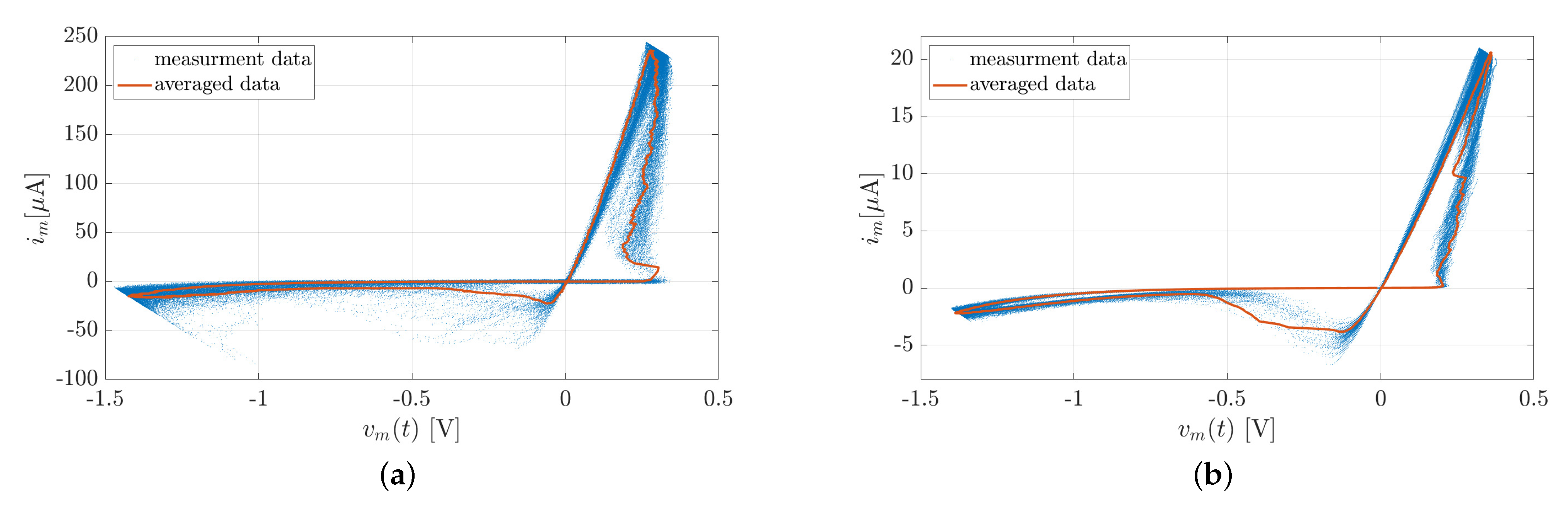
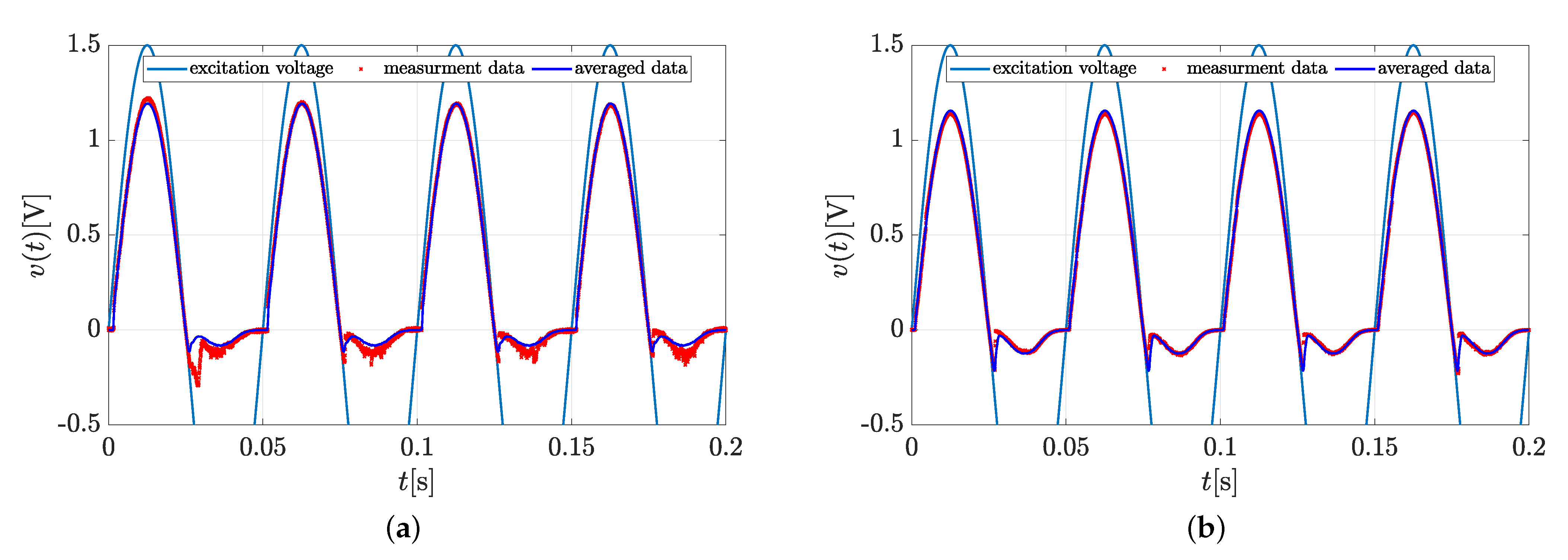
Applying the setup described in Section 3.1, the data have been acquired. For each combination of excitation voltage amplitude, the shape and frequency author always acquired data points, applying the rate of acquisition to the level where 100 periods of the response signal were always measured. For example, for the rate of acquisition was . During the measurement, some level of error has been observed. The Savitzky–Golay filter [21] has been applied to remove errors related to high frequencies components in the acquired data. To prepare the reference signal 1000 points from a single period of the output signal have been estimated. The estimation was the average signal over all 100 acquired periods of the signal. In Figure 2, one can find the example plot of the measured data compared with the averaged data. The plot represents the acquired data excited with the sinusoidal wave voltage of the amplitude and frequency . A typical hysteresis loop can be observed. One can also note two straight lines crossing the domain at the origin. These lines represent the high and low memristor resistances. Note that the transition is more stable in case of switching to LRS (the low resistance state). In general, the device with a carbon dopant has better stability then with the tungsten doping agent. This is also observed in Figure 3 where first four periods of the acquired data are shown. The averaged data are repeated over each presented period for comparison purposes. Furthermore the excitation data are limited for better visibility of the figure.
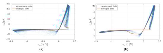
Figure 2.
plot of the measurement and the reference averaged data of the memristors with two kind of dopants. (sine wave, and ). (a) Tungsten dopant; (b) Carbon dopant.
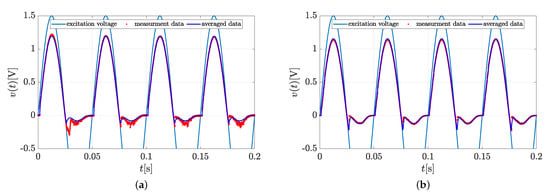
Figure 3.
Acquired time signals for the for the first 4 periods corresponding to the plots presented in Figure 2. (a) Tungsten dopant; (b) Carbon dopant.
3.3. Results Discussion
For understanding the quality of acquired data, some statistical factors have been proposed. To compare the acquired data for each period j (in this work ) with the averaged data the standard deviation normalized over the average value factor can be formulated as:
where is the number of data points in one period, and at the j-th period and are the i-th acquired and averaged voltage data points accordingly (). To estimate the error over all periods of the sample, another quadratic mean factor is proposed and defined as:
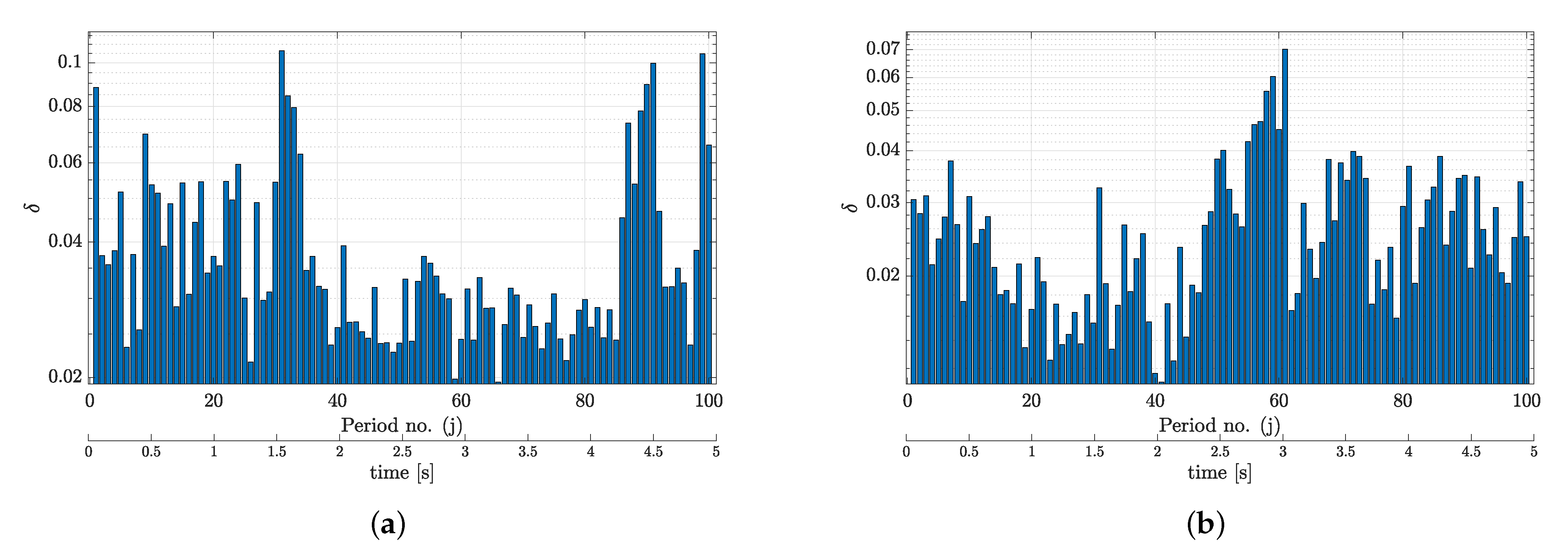
where m is the number of acquired periods of the measured signal (in this work ), and and are defined in Equation (8). For example, in Figure 4 the distribution of the deviation factor defined in (8) over each j-th period is presented. The graphs correspond to the samples presented in Figure 2. For better visibility the axis is in logarithmic scale. The maximum deviation is bigger for tungsten than for the memristor with carbon dopant. The graphs also show the quite big probabilistic behavior of the memristive elements. For the tungsten doped element, the maximum and minimum values of the deviation factor is 0.106491 and 0.019543 accordingly for 31st and 66th period. In case of carbon doping, these values are 0.070173 and 0.011106 for 61st and 41st period. It can be also noted that carbon doped element is more stable than doped with tungsten which can be measured using the error estimation defined in (9): and .
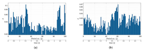
Figure 4.
Distribution of the deviation factor for the measured data. The graphs correspond to the samples presented in Figure 2. (a) Tungsten dopant; (b) Carbon dopant.
In Table 1, one can find all the errors defined in Equation (9) for all possible combinations of the excitation signal. The worst sample is for the memristor with tungsten dopant and for a triangle signal of frequency and the amplitude where . The best of the acquired signal with is for the signal measured on memristor with carbon dopant and for sinusoidal excitation of the frequency and amplitude . Note that in the case of memristor with carbon dopant the higher frequency is, the device responds with better stability.

Table 1.
The values of the error defined in Equation (9) of the acquired signals for two tested kinds of memristors and different combinations of voltage amplitude, shapes, and frequencies of the excitation signals. The highest and lowest numbers are indicated with bold font type.
4. Optimization Procedure
In this section, the optimization procedure is going to be described. The goal of this procedure is to find the optimal fitting parameters of the described in Section 2 memristor models that minimize some cost function. Cost function compares the results obtained from the model simulation with the reference signal. The models considered have parameters either real or integer valued. Let and be, respectively, the vector of real- and integer-valued parameters of the selected model. The cost function is defined as:
where n is the number of points in the reference signal (here one signal period with data points), for is the current at point in the reference signal, and is the current at point computed using the model for the given optimal parameters and . The reference current is simply computed from the averaged voltage data divided by the linear series resistor .
During the optimization process, one needs to find the the optimal parameters that minimize the cost function . Those optimal parameters represent the best model fit to the acquired real memristor data. Parameters represented as reals and integers are treated differently. Optimal real-valued parameter represented by the vector is determined for fixed integer-valued parameter . This process is carried out for all integer-valued parameters from the proposed set from the fixed range. The vector and minimizing the cost function Equation (10) is chosen as the optimal solution. The integer-valued parameters range from 1 to 10. Therefore, in the case of the asymmetric Strukov model and the VTEAM model, this means that the optimization process has to be repeated 100 times, which significantly extends the computation time. Similarly to the integer-valued parameters, the real-valued parameters are also subject to some box constrains. As the excitation signal is described by the continuous and periodic function, then the clearly modeled problem needs to be periodic in general. The internal state variables of the model also need to be expressed by the continuous function. To ensure that the continuity condition holds, the process of integration the dynamical part of the model is repeated until the condition is met, i.e., the transient time is finished and the system works in steady state. This condition requires to estimate an additional real-valued parameter that tells when the integration should start to get the memristor in steady state. All applied constraints to the real-valued parameters are indicated in Table 2.
Table 2.
Box constrains for the real-valued parameters of vector .
The interior-point algorithm [22] has been used in the optimization process. This algorithm is implemented as the fmincon function in the MATLAB optimization toolbox. This Matlab function is recommended for the optimization problems dealt in this work, it can handle the box constrains and the situations when the constraints are not valid or cannot be determined. Here the author noticed some problems with the internal variables continuity condition. In some cases, due to the lack of continuity condition, the fulfilling the cost function could not be determined, so this second Matlab function’s property was very useful. In [23], it was shown that the standard explicit Runge–Kutta (4,5) formula, which is implemented in Matlab as ode45 demonstrates some numerical errors while integrating the examined models with some discontinuities. The first-order Euler method was used to simulate memristor models. The Euler method offers reasonably fast integration with controlled step size and can deal with the problems mentioned above.
5. Results
In this section, the results of the optimization process are presented and discussed. The accumulated results are presented in Table 3. The best and worst modeled memristors for each model are indicated with the pink background. The memristor models are nonlinear, so the cost function (10) is also strongly nonlinear. Obtained results usually are rather local and it would be very hard to obtain the global minimum. Thus, the performance of the optimization procedure strongly depends on the initial point in the possible solution space provided to the algorithm. The initial points are prepared by hand performing some optimization tests before and then fixed for one model with all combinations of measurement data.
Table 3.
The results of the optimization procedure over all models considered. The maximum and minimum values of the cost function for each model are indicated with bold font type.
5.1. Strukov Model, Rectangular Window
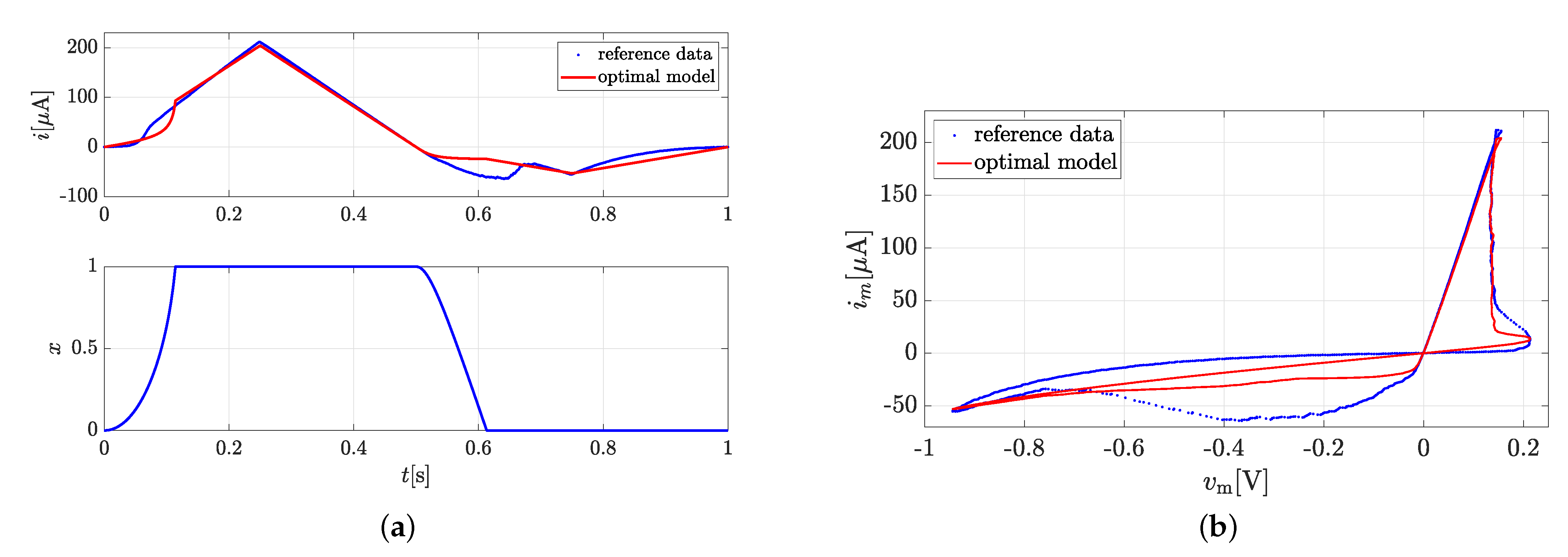
Comparison of the signal obtained from the optimal Strukov model with the rectangular window and the reference signal is presented in Figure 5 and Figure 6. The asymmetric Strukov model with rectangular window outperforms the symmetric Strukov model. The cost function value is times lower in case of the asymmetric model. The fitting parameters for the symmetric models are: , , and . For the asymmetric model, the parameters are: , , , and . The presented data for the best model are obtained using the Strukov model. From Table 3, one can notice that while the frequency increases, the model performance decreases and the proposed model is not sufficiently reflecting the real data.
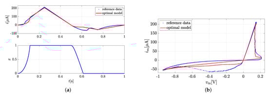
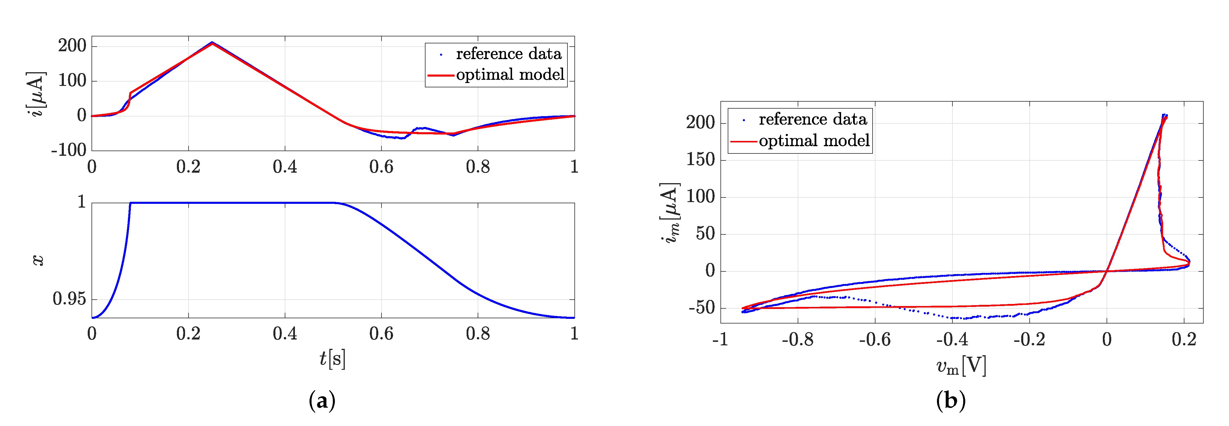
Figure 5.
Optimization results obtained for the Strukov model with rectangular window for memristor with tungsten dopant and triangle wave excitation voltage with and . . (a) Comparison graph of the memristor current obtained from the model and the reference data, and the internal variable ; (b) Corresponding plot.
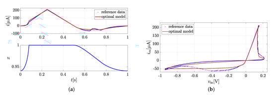
Figure 6.
Optimization results obtained for the asymmetric Strukov model with rectangular window for the same reference data presented in Figure 5. . (a) Comparison graph of the memristor current obtained from the model and the reference data, and the internal variable ; (b) Corresponding plot.
5.2. Strukov Model, Biolek Window
Comparison of the signal obtained from the optimal Strukov model with the Biolek window and the reference signal is presented is Figure 7. The reference data are obtained for a carbon doped memristor with the sine wave of the applied excitation voltage with the frequency and the amplitude . The obtained fitting parameters are: , , , and . This result can be compared with the asymmetric model which is presented in Figure 8 where the obtained fitting parameters are: , , , , , and . The cost function value for the asymmetric model is 15% lower then for the symmetric model. Unfortunately, as for Strukov with a rectangular window, it can be observed from Table 3 that when the frequency of the signal increases, the model performance decreases. Additionally, it has to be pointed out that in general, the asymmetric model is not always better than the symmetric one and the fitting cost function values are on similar levels.
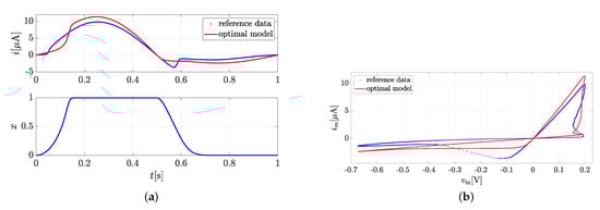
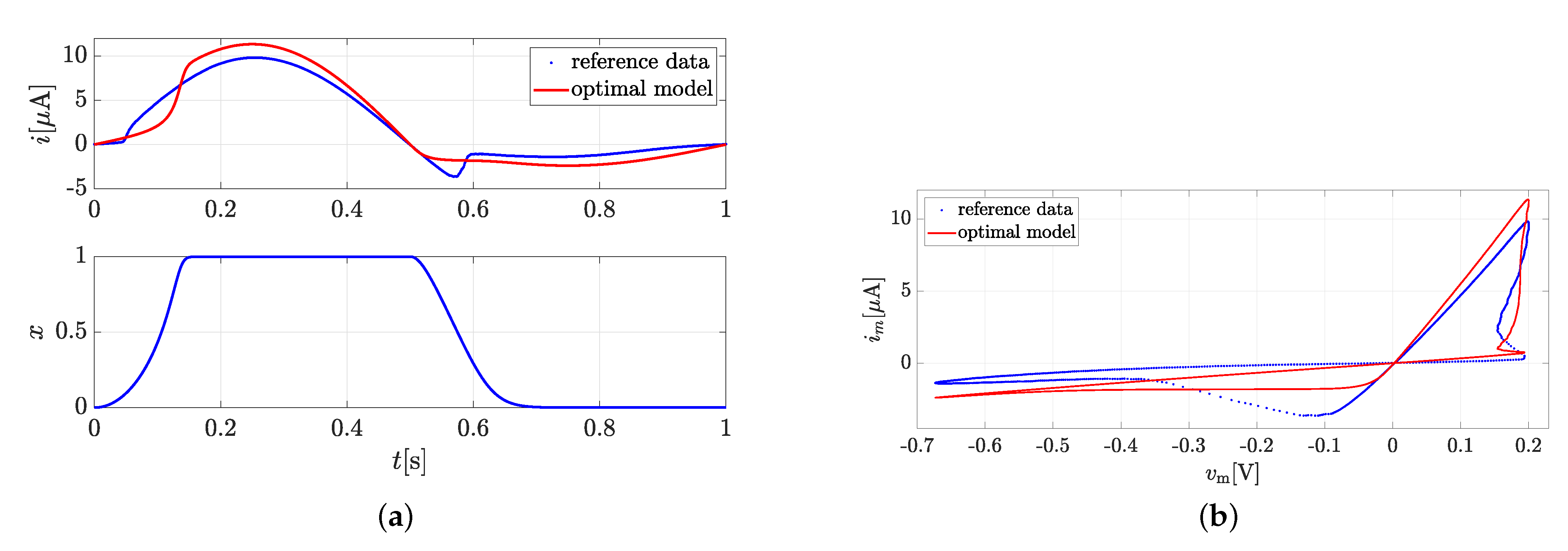
Figure 7.
Optimization results obtained for the Strukov model with Biolek window for memristor with carbon dopant and sine wave excitation voltage with and . . (a) Comparison graph of the memristor current obtained from the model and the reference data, and the internal variable ; (b) Corresponding plot.
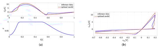
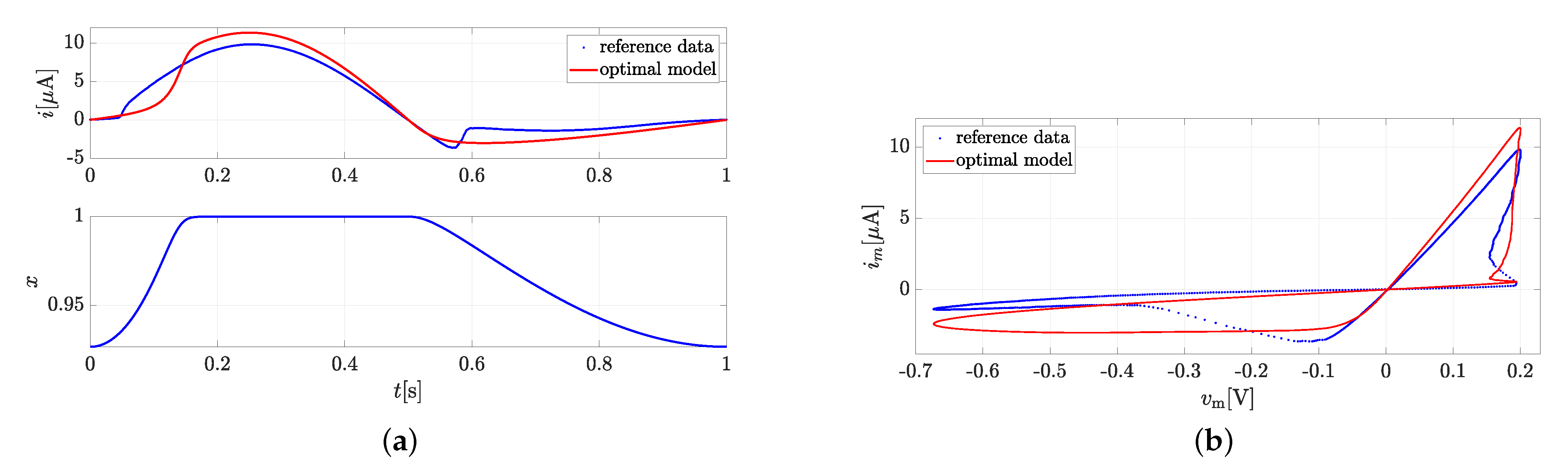
Figure 8.
Results of the optimization using the asymmetric Strukov model with Biolek window for the same reference data presented in Figure 7. . (a) Comparison graph of the memristor current obtained from the model and the reference data, and the internal variable ; (b) Corresponding plot.
5.3. VTEAM
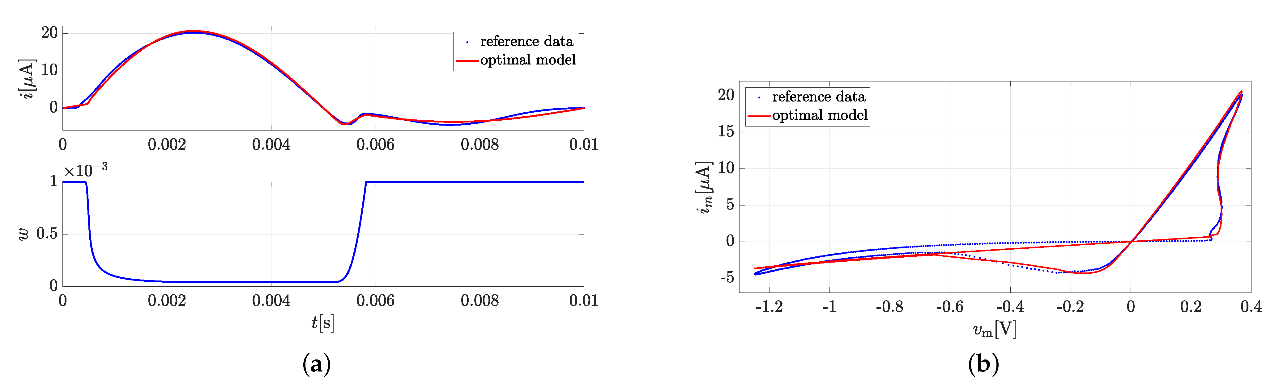
Figure 9 presents the comparison plot of the solution using the VTEAM model and the reference data. The fitting parameters of the model are: , , , , , , , and . In this case the value of the cost function is significantly lower than the result from the rest of the considered models. In general, the VTEAM model fits much better then the other models considered in this work. One needs always to remember that the solution might be better if different initial points are provided to the optimization algorithm.

Figure 9.
Optimization results obtained for the VTEAM model for memristor with carbon dopant and sine wave excitation voltage with and . . (a) Comparison graph of the memristor current obtained from the model and the reference data, and the internal variable ; (b) Corresponding plot.
5.4. Model Performance with Varying Frequency
In this subsection, the behavior of the VTEAM model is studied when frequencies of the input signal are varied. The authors consider the VTEAM model only as it outperforms the other considered models. The optimal model obtained for a given frequency is applied to other frequencies. The results are presented in Table 4. The model is optimized for the fixed frequency f reported in the third column of Table 4. The values of the cost function obtained for other frequencies are presented in the following columns. All this is presented for all combinations of the excitation voltage and the type of memristor dopant. In general, it can be noticed that the cost function values for the frequency combinations laying outside the diagonals are higher. It is interesting that there are some exceptions, e.g., for the tungsten doped memristor and with triangle excitation voltage of amplitude the performance of the model with the parameters obtained for frequency and applied to the data of the frequencies , and performs even better then for original one. There are also some worse scenarios. For example, the carbon doped memristor with sine voltage function and the parameters obtained for frequency applied to produce almost a 600 times worse fit compared to the reference data.
Table 4.
Cost function values if the optimal model parameters obtained for certain frequency are applied for the data of different frequency. The VTEAM model is considered.
6. Conclusions
The main goal of this work was to check the performance of the memristor models. As possible memristor applications are very wide, scientists and engineers expect a model that can provide some level of certainty independent of the excitation conditions. In the modeled devices, one can observe the bistability phenomenon. The problem is the transient state when the memristor switches. From the collected data, one can observe that switching from the HRS to LRS is more stable, but when the state changes in the opposite direction, one can find a much bigger stochastic behavior. Memristors with a carbon doping agent seem to be more stable than the device doped with tungsten. However, it is an interesting fact that the stability is on the higher level in comparison with the Pt/HfO/Ti/Pt memristor [24]. This uncertain behavior is modeled using some stochastic models [25,26,27,28]. There are some interesting approaches for the stochastic models adding the additional noise source [29,30,31]. It was also noticed that the considered noise and periodic signals can generate much more interesting and complex phenomena [32]. This manifests as an additional memristor property of stochastic multistable nonlinear systems. In the author’s opinion, this is interesting, but on the other hand this approach can model the element only with the certain fixed data measurement. Actually, the electronic engineers dispose of the appropriate models for standard electronic devices like diodes, transistors, operational amplifiers etc. The main goal of the model is to be as general as possible and it should fit to the modeled device under a big variety of excitation signals or even physical conditions. That is why in this work some memristor models have been tested. The response of the model parameters obtained for one frequency to the other frequency has also been analyzed. The result looks to be promising. In some cases, the performance is weak but there are also some contrary positive examples.
In this work, it has been shown that among all memristor models considered, the VTEAM model significantly outperforms the other ones. This conclusion can be seen analyzing the data presented in Table 5 where the average cost function values of the models are presented grouped by the excitation voltage, wave shape, and the doping agent. The threshold idea was the right choice to model the memristor behavior; on the other hand, the proposed asymmetric models do not increase significantly the model performance. It can be noticed that in the case of Strukov model with Biolek window, the symmetric model is even a little better then the asymmetric one for the case of memristor with tungsten dopant. Moreover, it has to be mentioned that in general, the Strukov model performance is limited to the frequency in the low range.
Table 5.
Average cost function values for all tested models grouped by the doping agent and the wave shape of the excitation voltage.
In the future work, authors can introduce some amendments to the tested models and apply the multi-objective optimization approach to improve their performance over a wider frequency range. The improvement of the measurement set-up is going to be introduced to avoid some data acquisition errors, especially for low currents. The author is going to implement the achieved results to test the memory devices as multi-bit memory cells.
The total results of the models with their fitting parameters are not presented in this work for paper clarity, but they can be provided by the author on any request.
Funding
The researches presented in the paper were financed by the Polish Ministry of Science and Higher Education, by a subvention of AGH University of Science and Technology, Krakow, Poland.
Institutional Review Board Statement
Not applicable.
Informed Consent Statement
Not applicable.
Data Availability Statement
Not applicable.
Acknowledgments
This work has benefited from discussions and advises from Zbigniew Galias from the AGH UST.
Conflicts of Interest
The author declares no conflict of interest.
References
- Strukov, D.B.; Snider, G.S.; Steward, D.R.; Williams, R.S. The missing memristor found. Nature 2008, 453, 80–83. [Google Scholar] [CrossRef] [PubMed]
- Pal, S.; Gupta, V.; Ki, W.H.; Islam, A. Design and development of memristor-based RRAM. IET Circuits Devices Syst. 2019, 13, 548–557. [Google Scholar] [CrossRef]
- Nugent, M.A.; Molter, T.W. AHaH Computing-From Metastable Switches to Attractors to Machine Learning. PLoS ONE 2014, 9, e85175. [Google Scholar] [CrossRef] [PubMed]
- Faridi, J.; Ansari, M.S. Memristor-Based Tunable Analog Filter for Physiological Signal Acquisition for Electrooculography. In Smart Technologies and Innovation for a Sustainable Future; Al-Masri, A., Curran, K., Eds.; Springer International Publishing: Berlin/Heidelberg, Germany, 2019; pp. 237–242. [Google Scholar]
- Corinto, F.; Lanza, V.; Ascoli, A.; Gilli, M. Synchronization in networks of FitzHugh-Nagumo neurons with memristor synapses. In Proceedings of the 2011 20th European Conference on Circuit Theory and Design (ECCTD), Linkoping, Sweden, 29–31 August 2011; pp. 608–611. [Google Scholar]
- Paprocki, B.; Pregowska, A.; Szczepański, J. Optimizing information processing in brain-inspired neural networks. Bull. Pol. Acad. Sci. Tech. Sci. 2020, 68, 225–233. [Google Scholar]
- Zhang, Y.; Wang, Z.; Zhu, J.; Yang, Y.; Rao, M.; Song, W.; Zhuo, Y.; Zhang, X.; Cui, M.; Shen, L.; et al. Brain-inspired computing with memristors: Challenges in devices, circuits, and systems. Appl. Phys. Rev. 2020, 7, 011308. [Google Scholar] [CrossRef]
- Chua, L.O. Memristor-the missing circuit element. IEEE Trans. Circuit Theory 1971, 18, 507–519. [Google Scholar] [CrossRef]
- Chua, L.O. Everything You Wish to Know About Memristors However, Are Afraid to Ask. Radioengineering 2015, 24, 319–368. [Google Scholar] [CrossRef]
- Sah, M.P.; Adhikari, S.P.; Kim, H.; Chua, L.O. Fingerprints of a memristor. In Proceedings of the 14th International Workshop on Cellular Nanoscale Networks and their Applications (CNNA), Notre Dame, IN, USA, 29–31 July 2014. [Google Scholar]
- Pershin, Y.V.; Ventra, M.D. Spin memristive systems: Spin memory effects in semiconductor spintronics. Phys. Rev. B Condens. Matter 2008, 78, 113–127. [Google Scholar] [CrossRef] [Green Version]
- Jo, S.H.; Kim, K.H.; Lu, W. Programmable resistance switching in nanoscale two-terminal devices. Nano Lett. 2009, 9, 496–500. [Google Scholar] [CrossRef]
- Chanthbouala, A.; Garcia, V.; Cherifi, R.O.; Bouzehouane, K.; Fusil, S.; Moya, X.; Bibes, M. A ferroelectric memristor. Nat. Mater. 2012, 11, 860–864. [Google Scholar] [CrossRef]
- Campbell, K.A. The Self-directed Channel Memristor: Operational Dependence on the Metal-Chalcogenide Layer. In Handbook of Memristor Networks; Chua, L., Sirakoulis, G.C., Adamatzky, A., Eds.; Springer International Publishing: Berlin/Heidelberg, Germany, 2019. [Google Scholar]
- Campbell, K.A. Self-directed channel memristor for high temperature operation. Microelectron. J. 2017, 59, 10–14. [Google Scholar] [CrossRef]
- Kvatinsky, S.; Ramadan, M.; Friedman, E.G.; Kolodny, A. VTEAM: A general model for voltage-controlled memristors. IEEE Trans. Circuit Syst. II Express Briefs 2015, 62, 786–790. [Google Scholar] [CrossRef]
- Biolek, Z.; Biolek, D.; Biolkowa, V. SPICE model of memristor with nonlinear dopant drift. Radioengineering 2009, 18, 210–214. [Google Scholar]
- Corinto, F.; Ascoli, A. A boundary condition-based approach to the modeling of memristor nanostructures. IEEE Trans. Circuits Syst. I 2012, 59, 2713–2726. [Google Scholar] [CrossRef]
- Joglekar, Y.N.; Wolf, S.J. The elusive memristor: Properties of basic electrical circuits. Eur. J. Phys. 2009, 30, 661–675. [Google Scholar] [CrossRef] [Green Version]
- Garda, B.; Galias, Z. Modeling of memristors under sinusoidal excitation with various frequencies. In Proceedings of the 25th IEEE International Conference on Electronics, Circuits and Systems, Bordeaux, France, 9–12 December 2018. [Google Scholar]
- Savitzky, A.; Golay, M.J.E. Smoothing and Differentiation of Data by Simplified Least Squares Procedures. Anal. Chem. 1964, 36, 1627–1639. [Google Scholar] [CrossRef]
- Byrd, R.H.; Mary, E.H.; Nocedal, J. An Interior Point Algorithm for Large-Scale Nonlinear Programming. SIAM J. Optim. 1999, 9, 877–900. [Google Scholar] [CrossRef]
- Galias, Z. Simulations of memristors using the Poincaré map approach. IEEE Trans. Circuits Syst. I 2020, 67, 963–971. [Google Scholar] [CrossRef]
- Garda, B.; Kasiński, K.; Ogorzałek, M.; Galias, Z. Investigations of switching phenomena in Pt/HfO2/Ti/Pt memristive devices. In Proceedings of the 2017 European Conference on Circuit Theory and Design (ECCTD), Catania, Italy, 4–6 September 2017. [Google Scholar]
- Hu, M.; Wang, Y.; Qiu, Q.; Chen, Y.; Li, H. The stochastic modeling of TiO2 memristor and its usage in neuromorphic system design. In Proceedings of the 2014 19th Asia and South Pacific Design Automation Conference (ASP-DAC), Singapore, 20–23 January 2014; pp. 831–836. [Google Scholar]
- Naous, R.; Al-Shedivat, M.; Salama, K.N. Stochasticity Modeling in Memristors. IEEE Trans. Nanotechnol. 2016, 15, 15–28. [Google Scholar] [CrossRef] [Green Version]
- Molter, T.W.; Nugent, M.A. The Generalized Metastable Switch Memristor Model. In Proceedings of the 15th International Workshop on Cellular Nanoscale Networks and their Applications (CNNA), Dresden, Germany, 23–25 August 2016. [Google Scholar]
- Stathopoulos, S.; Serb, A.; Khiat, A.; Ogorzałek, M.; Prodromakis, T. A Memristive Switching Uncertainty Model. IEEE Trans. Electron Devices 2019, 66, 2946–2953. [Google Scholar] [CrossRef] [Green Version]
- Filatov, D.O.; Vrzheshch, D.V.; Tabakov, O.V.; Novikov, A.S.; Belov, A.I.; Antonov, I.N.; Sharkov, V.V.; Koryazhkina, M.N.; Mikhaylov, A.N.; Gorshkov, O.N.; et al. Noise-induced resistive switching in a memristor based on ZrO2(Y)/Ta2O5 stack. J. Stat. Mech. Theory Exp. 2019, 2019, 124026. [Google Scholar] [CrossRef]
- Agudov, N.V.; Safonov, A.V.; Krichigin, A.V.; Kharcheva, A.A.; Dubkov, A.A.; Valenti, D.; Guseinov, D.V.; Belov, A.I.; Mikhaylov, A.N.; Carollo, A.; et al. Nonstationary distributions and relaxation times in a stochastic model of memristor. J. Stat. Mech. Theory Exp. 2020, 2020, 024003. [Google Scholar] [CrossRef] [Green Version]
- Agudov, N.V.; Dubkov, A.A.; Safonov, A.V.; Krichigin, A.V.; Kharcheva, A.A.; Guseinov, D.V.; Koryazhkina, M.N.; Novikov, A.S.; Shishmakova, V.A.; Antonov, I.N.; et al. Stochastic model of memristor based on the length of conductive region. Chaos, Solitons Fractals 2021, 150, 111131. [Google Scholar] [CrossRef]
- Baranova, V.N.; Filatov, D.O.; Antonov, D.A.; Antonov, I.N.; Gorshkov, O.N. Resonant activation of resistive switching in ZrO2(Y) based memristors. J. Phys. Conf. Ser. 2020, 1695, 012151. [Google Scholar] [CrossRef]
Publisher’s Note: MDPI stays neutral with regard to jurisdictional claims in published maps and institutional affiliations. |
© 2021 by the author. Licensee MDPI, Basel, Switzerland. This article is an open access article distributed under the terms and conditions of the Creative Commons Attribution (CC BY) license (https://creativecommons.org/licenses/by/4.0/).