Deduction of Optimal Control Strategies for a Sector-Coupled District Energy System

Abstract

We present a method to turn the results of model-based optimisations into resilient and comprehensible control strategies. Our approach is to define priority lists for all available technologies in a district energy system. Using linear discriminant analysis and the results of the optimisations, these are then assigned to discrete time steps using a set of possible steering parameters. In contrast to the model-based optimisations, the deduced control strategies do not need predictions or even perfect foresight but solely rely on data about the present. The case study using priority lists presents results in terms of emissions and prices that are only about 5% off the linear optimum. Considering that the priority lists only need information about the present, the results of the control strategies obtained using the proposed method can be considered competitive.

1. Introduction

To achieve the 1.5 ${}^{\circ }$C ([1], p. 21) goal of the Paris Agreement, immediate action is strongly advisable [2,3,4]. On short timescales, changed operation can contribute to significant reductions of emissions. For example, a district heating supply using heat pumps and a thermal energy storage could reduce emissions by 20% only due to an adjusted operation strategy ([5], pp. 10–15).

For longer time scales, integration of the electricity sector with other sectors is a key measure. There are two reasons for this: Low-emission electricity sources such as wind farms, photo voltaic, and nuclear power plants are technically available and can be used for industry, mobility, and heat [6,7,8,9]. On the other hand, the electricity sector can also benefit from the integration, i.e., the sector coupling can provide flexibility [10,11].

The underlying problem can be solved using various methods [12], i.e., by modelling the energy system followed by an optimisation based on predictions [13]. However, most methods are rather complex and computation-intensive, depending, e.g., on machine learning [14,15,16]. Thus, we see a need for less data-intensive and more comprehensible control strategies that can provide competitive solutions even if forecasts are (temporarily) unavailable. Existing control strategies increase the capability for local operation that is independent of data-intense simulations and thus enhance a more resilient ([17], p. 253) operation of energy systems.

Our approach is to deduce simple control strategies from the results obtained in model-based optimisations. Having in mind the advantages of integrated energy systems, the method should be usable with them. Thus, we present a case study along with our method. It applies the newly developed method to a combined heat and power (chp) based system. To also highlight the general potential of reducing green house gas (ghg) emissions by changing control strategies, the case study implements optimisation for both economic costs as well as ghg emissions.

The context of the case study is set in a project called ‘Energetisches Nachbarschaftsquartier’ (short ENaQ, Energetic Neighborhood Quarter), which focuses on developing a district for about 140 households in Oldenburg, Germany, including supply with heat and electricity.

With the deduction, we obtain control strategies that are resilient and comprehensible. Resilient in this context refers to the independence of forecasts and computation- and data-intensive simulations: The operation with the deduced control strategies does not need any model optimisation or perfect foresight anymore. Comprehensible in this context refers to the goal of a control strategy that actors of the implementation of local energy supply systems can intuitively understand and thus puts the power of goal evaluation in the hands of these actors. Comprehensible control strategies are contrasted by more complex model-based optimisations and simulations for the control of the operation. Our solution is an equation that converts time-specific values of steering parameters in a priority list of technologies that can supply the demand:

$$z=\sum _i{w}_i\times x_i$$

(1)

In Equation (1), the steering parameters $x_i$ get weights $w_i$ and are converted to a value z. With cut-off-values, each value for z represents a class and each class represents a priority list of the available technologies. These priority lists can control the operation of the local energy supply system so that emissions of and prices for the operation are comparable to the ones obtained with the linear optimisation.

With the proposed control strategies, data and computation intensity as well as the need for prediction in operation are reduced. Additionally, priority lists as control strategies could reduce the need for models and simulations and therefore make elaborate control strategies available for a wider range of actors. This would become possible as soon as the control strategies are not deduced from linear model optimisations. With our paper, we show that the control strategies perform almost as well as model-based optimisations and thereby lay the foundation for further work in that direction.

The overall methodology is shown in Figure 1. An important hypothesis for the method is that priority lists can describe model-optimised control strategies. So first, in Section 2.1, we argue why we think that this is actually the case. Afterwards, we explain our deduction method in Section 2.2. Section 3 contains our case study. Here, we start by introducing our energy system design and the linear model optimisation (Section 3.1). In Section 3.2, we then walk through the deduction of control strategies based on the given example. In Section 3.3, we present results of the case study. These results underline the applicability and potential of the method. Finally, we give an overview of our most important research boundaries in Section 3.4.

2. Method for the Deduction of Control Strategies

2.1. Priority Lists Describing Optimal Control Strategies

We express the energy system by a directed graph connecting sources and sinks via various other nodes. The sinks model a fixed energy demand ${\Delta }_t\times P_s\left(t\right)$, while the energy supply from the sources can be flexible. The edges, connecting the nodes, have three properties,

• $c_e\left(t\right)$, the cost (in Units per Joule);
• ${\eta }_e>0$, the transmission efficiency;
• $P_{\max ,e}\left(t\right)>0$, the maximum power (in Watts).

Now, a linear optimiser can be used to find

$$\mathrm{argmin}\sum _e{c}_e\left(t\right)\times P_e\left(t\right),$$

(2)

the optimal control strategy that minimises the cost.

If there is just one sink and the graph is acyclic (loop-free), it is trivial that alternatively a list can be created that orders all possible supply options (all paths connecting the sources and the sink) by their cost. When starting from the cheapest option, this priority list also gives the optimal supply solution.

Note that for any technical system ${\eta }_e<1\forall e$, provided that all sources are explicitly modeled. Thus, it is safe to assume that a loop-free representation exists: The contribution of infinite loops will vanish and finite loops can be unrolled.

If there are $N_{\mathrm{sink}}$ sinks with their respective $P_s\left(t\right)$ ($0<s\le N_{\mathrm{sink}}$), it is possible to replace them by N edges and one sink: The edges have $P_{\max ,s^{\prime }}\left(t\right)=P_s\left(t\right)$, and the new sink has a demand of $P\left(t\right)={\sum }_s{P}_s\left(t\right)$. This means, that the optimal solution of any directed acyclic graph can be expressed by a priority list of paths connecting the sources and the sinks. As the $P_{\max ,e}\left(t\right)<\infty$ and $c_e\left(t\right)>0$ are determined by ‘technologies’, this can be seen as a list of technologies.

Additionally, there might be linked edges with $P_e\left(t\right)\propto P_{e^{\prime }}\left(t\right),e\ne e^{\prime }$. In this case, the two paths count as one technology in the priority list. These complicate the creation of the priority list, but do not render the approach invalid: Consider the case of demand for heat and electricity, where electricity is for free but heat is provided cheapest by a combined heat and power plant: In this case, the chp will have priority. Additionally, note that creating the priority list is typically not as easy as sorting by costs. Consider the example of limited supply of electricity and a fixed demand of heat. Even if direct conversion (e.g., using a heating rod) was for free, a more costly option (e.g., a heat pump) might have priority to be even able to fulfill the demand.

In this context, storage marks a special kind of technology. It links different points in time, thus it can be expressed as a node in a graph that links the graphs for all time steps. Due to fact that a storage cannot be charged and discharged at the same point in time, the graph is still acyclic. However, the priority list would have to contain all possible paths for all points in time. Thus, this representation is not considered further. Instead, it can potentially sink our source—provided that a storage is neither full nor empty. Technically, this second representation also connects all points in time: only energy fed into the storage can eventually be drawn from it at a later point in time—if it is not lost due to storage inefficiencies or long holding times. Still, the error by neglecting this fact is small if the control strategy is appropriately chosen for the size of the storage [18].

To summarise, creating a priority list expressing the optimal control strategy is possible. However, it is not an easy task. Hence, we fall back to linear optimisation and create priority lists on that basis.

2.2. Deduction of Optimal Control Strategies: Classification Based on Steering Parameters

The first step of our method is the construction of an energy system model (cf. [19,20,21]). This model is then optimised with perfect foresight, e.g., using linear programming. From the model optimisations, we obtain energy flows that are optimal for the respective goal. These results are starting points of our deduction. Note that they still depend on various non-constant parameters, i.e., the energy demand and production of renewable energies depend on the weather. Thus, it is hard to work with them. To tackle this, the energy flows are normalised, yielding ‘capacity shares’. The capacity shares are values from 0% up to 100% that indicate how much of its potential a technology supplies to the local demand for a given time step. The capacity shares now help to identify which of the technologies are prioritised by the optimisation.

Now, we define all possible priority lists as classes in a classification problem [22]. If possible, we already reduce the numbers of classes at this stage. For example, if one supply option can fulfill the whole demand, the second and third priority do not matter.

Having this set of classes, we assign a class to each time step by the combination of capacity shares. Often, the priorities and thereby class can be assigned intuitively. In case two technologies are both in full-load-operation, it is harder to assign a class. To assign classes to these more difficult cases, we first assign the classes to the easy-to-assign conditions. Then, we evaluate the relative frequency of each of the classes. Based on these relative frequencies, we assign the difficult-to-assign conditions. We assign conditions to classes until all data points are assigned to one of the defined classes.

As already discussed in Section 2.1, storage needs special attention and we decided to include storage as two technology options, a source as well as a sink. Theoretically, this allows unreasonable combinations like charging and discharging at the same time, but of course the resulting classes can be easily eliminated. There are alternatives and we want to explain why we decided not to use them: First, it would also be possible to set a storage condition—charge, discharge or none—for each time step. This way, the storage is not included in the priority list, thus, part-load operation would be impossible or at least more difficult to express. A second alternative is assigning positive and negative values to all technologies in the priority lists for all conditions. Then, the storage could charge as long as the technologies supply above a defined positive value and discharge as long as no technology above a defined negative value supplies. This solution allows part-load operation but adds a lot of complexity as a sign that all technologies would need to be defined and deduced from the model optimisations.

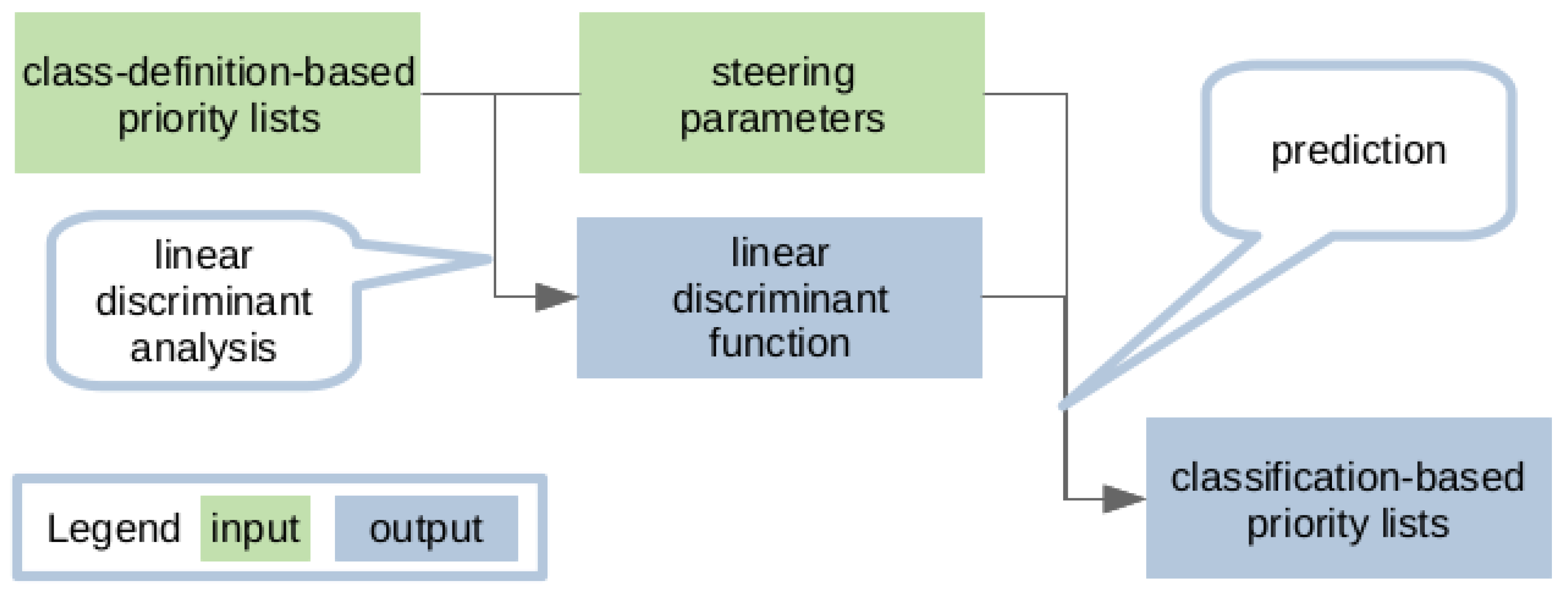
Having all conditions assigned to a class, we get priority numbers for all time steps and the relative frequencies of all fined classes for our example. These class-definition-based priority lists should deliver the same results as the model-optimisation according to our argumentation in Section 2.1—if we assign all time steps correctly. Finally, the assignment of classes to the state of the input parameters is done. For this, we use linear discriminant analysis (c.f. Figure 2). The resulting classification-based priority lists consist of factors to the input parameters (see Equation (1)) as well as the cutoff values, that can then be used to control the local energy supply system.

3. Case Study: CHP Based Heat Supply

3.1. Energy System Design and Linear Optimisation

As a practical example for the method described above, we present the following case study. First, we need an energy system model to optimise. We model a residential energy supply system using the open energy modeling framework (oemof) [23,24] packages solph [25] and thermal, following the methodology of the Model Template for Residential Energy Supply System (MTRESS) [26,27]. For the actual optimisation, the solver COIN-OR Branch and Cut (Cbc) [28,29] is used.

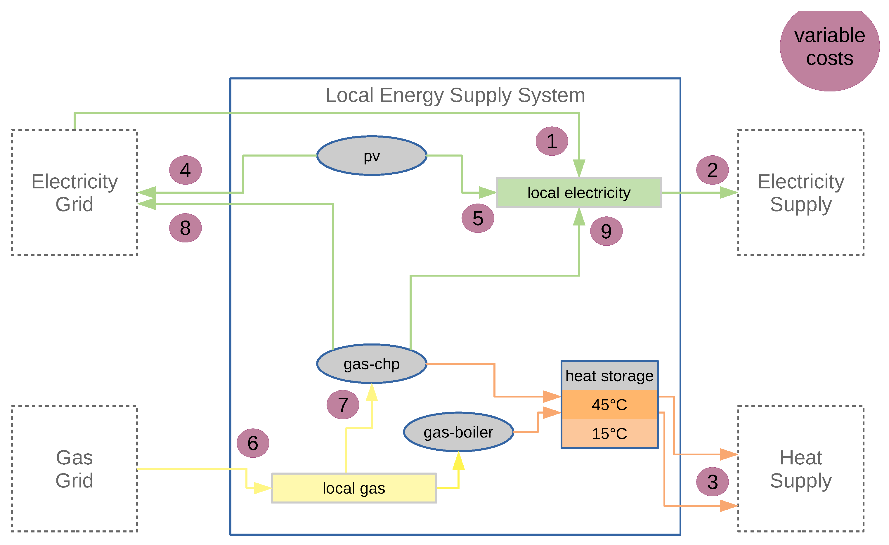
In Figure 3, the local energy supply system is shown. It consists of a photovoltaic (pv) system with an installed capacity of 100 kW, a cylindrical heat storage of 7 m height and a volume of 50 m3 with 10 cm of insulation with a thermal conductance of $0.04$ W/(mK). For the losses, we assume a stratified distribution of heat with a moving boundary [30]. Heat can be supplied by either a gas boiler (unlimited power) or a gas powered chp. The latter has an operational range between 53 kW and 85 kW with respect to thermal power and between 25 kW and 50 kW for electrical power. 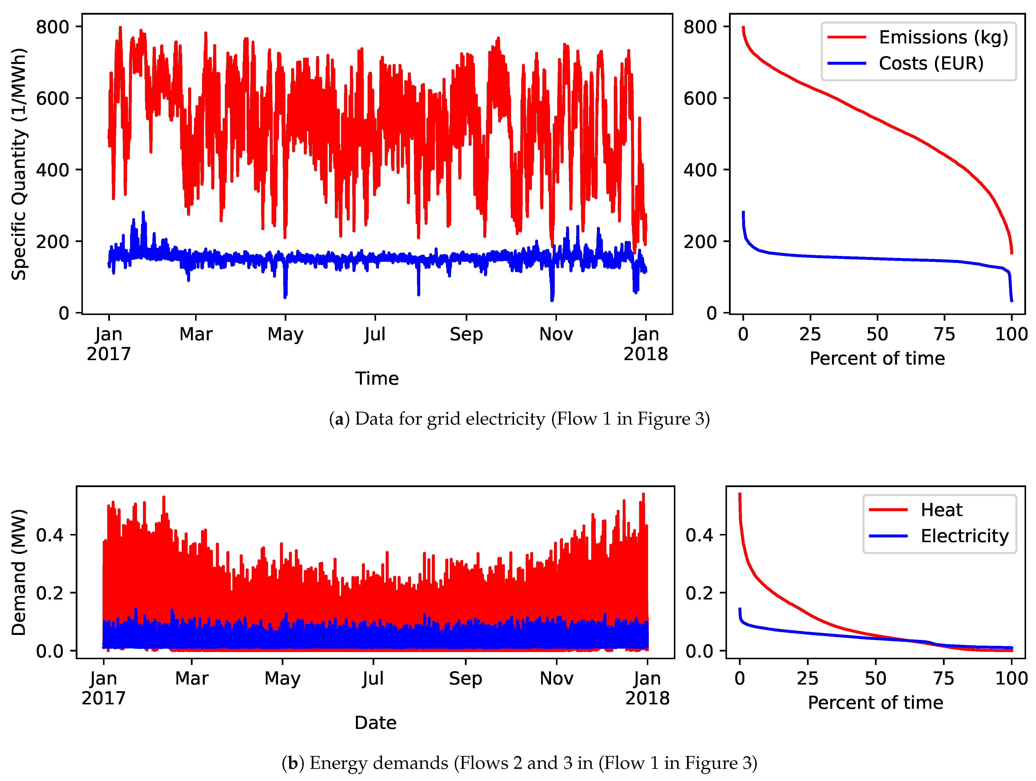For the gas from the grid, emissions are assumed to be constant at 201 kg/MWh [31], costs are $42.57$ EUR/MWh [32]. For time series, we use historical data of 2017 as in the region this is the last year that had several weeks of frost. Although it might be questioned if this former typical weather is still standard for average winters, we wanted it to be covered. The time resolution is 1 h. Emissions are calculated using flow tracing [33], for the prices, constant levies plus day ahead market prices are used (2017, region DE-AT-LU [34], see Figure 4a). The revenue for electricity from the gas-powered chp plant also depends on time, as constant subsidies are paid on top of the day ahead market prices. All considered costs (emissions or prices) are summarised in

Table 1. Specific costs assumed in the model.

Cost	Emissions [kg/MWh]	Price [EUR/MWh]
$c_1$	167…797	34.07…280.65
$c_2$	0	−249.84
$c_3$	0	−50.00
$c_4$	0	−72.90
$c_5$	0	67.56
$c_6$	201	42.57
$c_7$	0	−5.50
$c_8$	0	−243.52…3.06
$c_9$	0	27.56

. Note that the time-dependent values can only be assumed to be fixed if the local supply system is small with respect to the overall supply and demand in the grid.

The yearly demand for electricity is 376 MWh. The heat demand is split into a demand for heating of 402 MWh and a demand for domestic hot water of 336 MWh. These values are realistic for newly built multi family build homes with about 150 apartments as we assume them for ENaQ [33].

To illustrate the potential changing of the control strategy, we conduct two separate optimisations, one for emissions and one for prices. For the given scenario, the lowest possible emissions are 237 kg/MWh with a complementing revenue of $61.93$ EUR/MWh. On the other hand, the maximum revenue is $68.66$ EUR/MWh with complementing emissions of 269 kg/MWh.

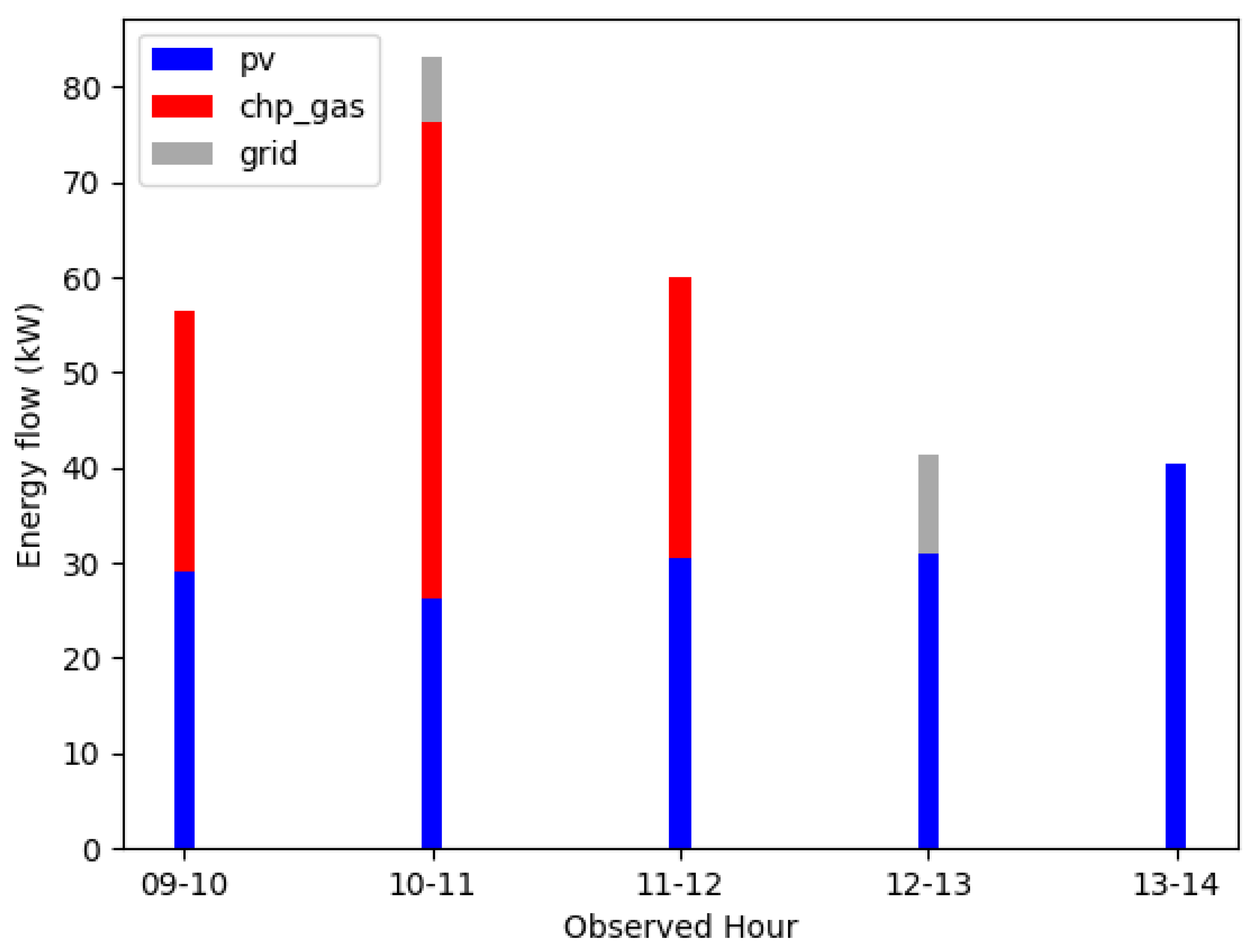
The starting point for the deduction of the control strategy are the details of these optimisations. Specifically, we obtain hour-specific energy flows for the different optimisation goals for the time frame of one year. In Figure 5, exemplary result data for some hours of a day for the electricity supply of the model-optimisation on emissions are shown. In the figure, energy sums in particular hours are shown—the sum of each hour represents the demand in this hour. The total electricity demand differs from hour to hour, in this case within 40 kWh and 84 kWh. The supply technologies for each hour are either pv and chp, pv, chp and grid, pv and grid, or only pv.

3.2. Classification for the Deduction of Control Strategies

From the results obtained by the optimising operation, we then deduce optimal control strategies. We do so by classification ([35], pp. 231–252) via linear discriminant analysis ([35], p. 235) with the implementation provided in Scikit-learn [36].

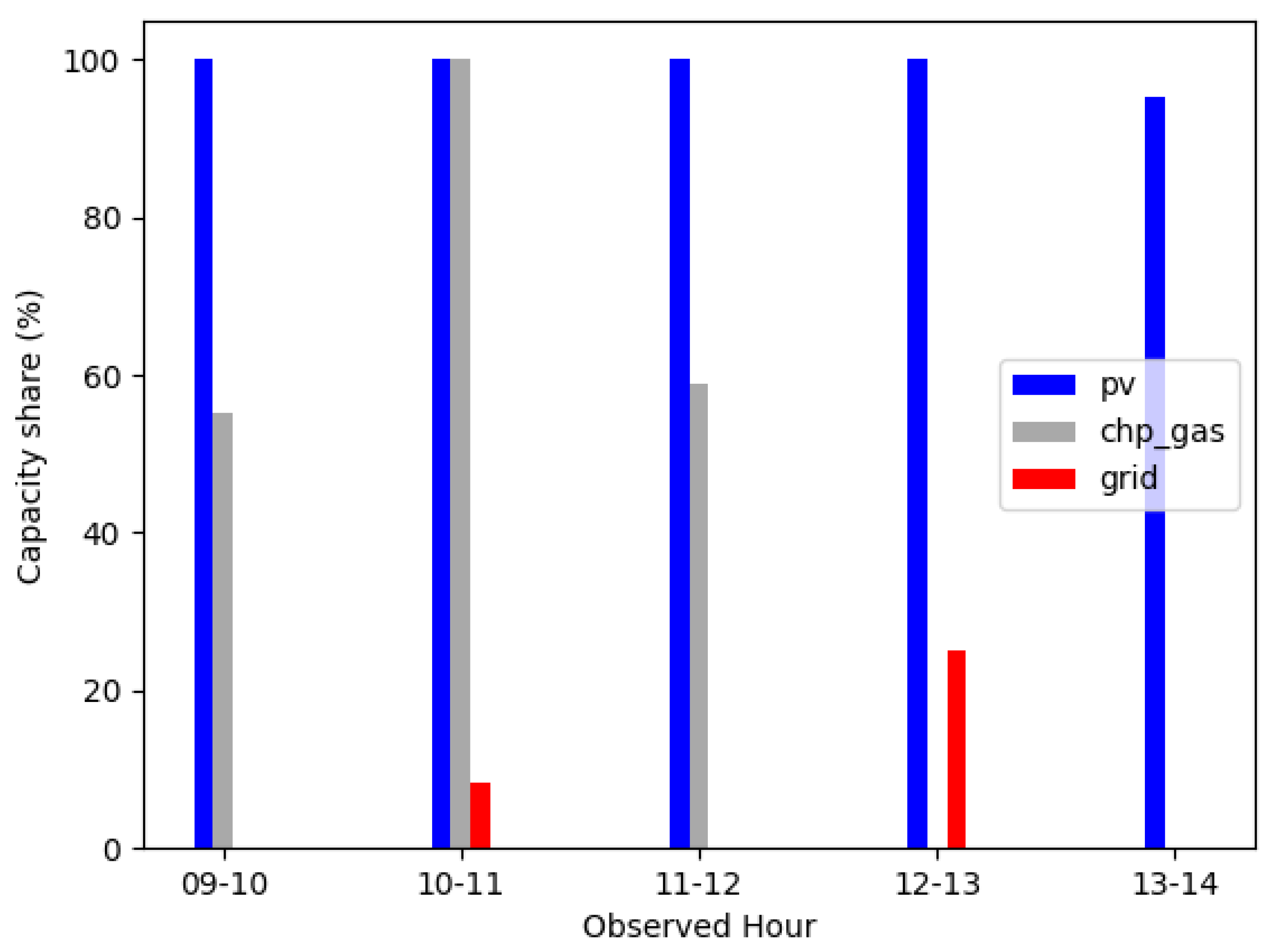
The energy flows from Figure 5 are transformed to the capacity shares shown in Figure 6. For photovoltaic (pv), the capacity is a time series depending on the irradiation. If there is no irradiation, we define the capacity share to be zero. For chp, the capacity is a fixed value in terms of installed capacity. For the grid, the capacity is equal to the demand.

These capacity shares help to identify which of the technologies are prioritised by the optimisation in each hour. In the following, we explain how we assign different situations in the energy system in terms of different capacity shares of the different technologies to technology-specific priority numbers.

We start by defining all possible in the form of priority lists. These classes are specific for heat and electricity supply. In

Table 2. Priority lists as defined classes (electricity).

Class	pv	chp	Grid
Class 1	1	2	3
Class 2	1	3	2
Class 3	2	1	3
Class 4	3	1	2
Class 5	2	3	1
Class 6	3	2	1

, we show the example of the electricity supply. If suitable, we already reduce the numbers of classes at this stage. For the given example, classes 5 and 6 do not both need to exist, because if the grid is preferred it can supply the full demand—therefore the second and third priority do not matter. So, we have already reduced the classes before assigning certain conditions of the energy system to them.

Having this set of classes, we assign a class to each time step via conditions. A condition is a certain set of capacity share combinations. In

Table 3. Example: assignment of classes with conditions of capacity share combinations.

Case	Condition	Share pv	Share chp	Share Grid	Class
A	pv full- and chp part-load	${\widehat{f}}_{\mathrm{pv}}=1$	$0<{\widehat{f}}_{\mathrm{chp}}<1$	${\widehat{f}}_{\mathrm{g}}<1$	1
B	pv full-load and chp off	${\widehat{f}}_{\mathrm{pv}}=1$	${\widehat{f}}_{\mathrm{chp}}=0$	${\widehat{f}}_{\mathrm{g}}<1$	2
C	pv part- and chp full-load	$0<{\widehat{f}}_{\mathrm{pv}}<1$	${\widehat{f}}_{\mathrm{chp}}=1$	${\widehat{f}}_{\mathrm{g}}=0$	3
D	pv and chp full-load	${\widehat{f}}_{\mathrm{pv}}=1$	${\widehat{f}}_{\mathrm{chp}}=1$	${\widehat{f}}_{\mathrm{g}}<1$	1 or 3 → 1

, two of these conditions are shown as an example for the electricity supply. The first example (A) is a full-load supply of the chp plant, part-load supply of the photovoltaic (pv) plant, and no supply from the grid. In the second example (B), the chp is not operated and some energy is coming from the electricity grid. Part-load of the photovoltaic (pv) plant is seen in case (C). This refers to some of its energy being exported to the grid. For all these cases, the priorities and thereby class can intuitively be assigned. In case of both technologies in full-load-operation (D), it is harder to assign a class.

Evaluating the relative frequency of each of the other classes, the most occurring class with the easy-to-assign conditions for the emissions-optimisation is class 1 and therefore we assign this condition to class 1 with pv prioritised over chp. We assign conditions to classes until all data points are assigned to one of the defined classes.

For the class definitions for the heat supply, we use the same method. The technologies for the heat supply are a gas-powered boiler, a gas-powered chp, and the charging or discharging heat storage.

Having all conditions assigned to a class, we get priority numbers for all time steps (

Table 4. Example priority numbers (1 is highest) derived from capacity shares (electricity).

Observed Hour	pv	chp	Grid
09–10	1	2	3
10–11	1	2	3
11–12	1	2	3
12–13	1	3	2
13–14	1	3	2

) and the relative frequencies of all defined classes for our example.

The results are specific for the supply of electricity and heat as well as the optimisation goal, in this case, the supply of electricity and optimisation on emissions. These class-definition-based priority lists should deliver the same results as the model-optimisation according to our argumentation in Section 2.1—if we assign all time steps correctly. The results are shown in

Table 5. Average emissions for one year of simulation and optimisation on emissions (in kg/MWh).

Linear	Class	Full	Electricity	Top Priority
Optimum	Assignment	Classification	Classification	Classification
237	250	253	251	298
( $100.0$%)	( $105.5$%)	( $106.8$%)	( $105.7$%)	( $125.6$%)

for emissions (Section 3.3.1) and

Table 6. Average prices for one year of simulation and optimisation on prices (in EUR/MWh).

Linear	Class	Full	Electricity	Top Priority
Optimum	Assignment	Classification	Classification	Classification
$-68.66$	$-67.22$	$-65.23$	$-60.71$	$-41.67$
( $100.0$%)	( $97.9$%)	( $95.0$%)	( $88.4$%)	( $60.7$%)

for prices (Section 3.3.2).

In order to only have one priority list, we combine the deduced optimal control strategies for electricity (three entries per time step) and heat (four entries per time step). In our case, the two priority lists are linked through the chp plant. As electricity can be supplied at different points in time with more or less s in terms of emissions and prices while the supply of heat has no changing costs (c.f. Figure 3), we decided to prioritise the decisions for the electricity technologies over the ones for the heat technologies. This way, we reduce the complexity of the class assignment for all conditions by reducing the number of technologies. For our particular energy system design, this complexity reduction is possible. However, for other energy system designs, a class assignment including all technologies might be necessary.

Using linear discriminant analysis, we then attribute the assigned classes to the different statuses of available input time series. In this pilot study, we also further reduce the number of classes by eliminating all but the first n priorities to find out how long the priority lists have to be in order to find reasonably good control strategies.

3.3. Validation and Results

In our validation, we compare the results of the model-optimisation and the results that we obtain with the deduced optimal control strategies. We do so for the results in terms of emissions for the emissions-optimisation and in terms of prices for the price-optimisation. We validate both the class-definition-based and the classification-based control strategies. The class-definition- and classification-based control strategies are deduced from the linear optimisation results but do not depend on linear optimisation, models or perfect foresight anymore. We also perform a sensitivity analysis of our classification-based control strategies. For the sensitivity analysis, we reduce the information of our priority lists. For the classification-based control strategies, we validate using the information on all seven priority numbers for heat and electricity. In a first step, we reduce the information to only the priority numbers for electricity and set all the priority numbers for heat to four. In a second step, we further reduce the information to only the first priority number and set all other priority numbers to two. This way, we want to see how many of our priority numbers have an impact on the results.

To validate the deduced optimal control strategies, we use the very same energy system model as for the optimisation. Here, we replace the costs in terms of emissions or prices by costs derived from the priority number (cf. Table 4). For electricity, we want higher differences between the priorities so that decisions for electricity outweigh those for heat. A possible formulation to assign a cost $c_i$ to a priority number $p_i$ is

$$c_i=-{10}^{-p_i}$$

for every time step. Practically, the non-equidistant stepping determines what to do when the combined heat and power (chp) has a high priority on one list and a low priority on the other one. Further note that we only choose this way to directly compare the methods within the same energy system model. In principle, the deduced control strategy does not rely on linear optimisation, thus the problem of assigning costs only occurs because of our validation method.

3.3.1. Performance in Terms of Emissions

In Table 5, the results in terms of emissions are shown. The linear optimum is obtained by the linear optimisation using the open energy modeling framework (oemof).solph. The results from this linear optimisation are the reference for the validation and therefore the $100.0$% on the relative scale. With the class assignment, we show the validation results that we obtain with the class-definition-based validation. These results are thus already obtained with priority lists as classes—but not yet with the priority lists that we obtain by the deduced control strategies from the linear discriminant analysis. In the classification, the results with the classification-based validation considering a different amount of priority numbers are shown.

In terms of emissions, the class-definition-based priority lists lead to $5.5$% higher emissions. This is not in line with our expectation of perfectly predictable priority lists. It indicates that our assignment of priority lists with conditions is not yet perfect, as we argue in Section 2.1 that an assignment should be possible. Nonetheless, $5.5$% higher emissions is still a result that supports the hypothesis that priority lists can be used as control strategies. For comparison: With the linear optimisation on prices, the emissions increase by $12.0$% when compared to the lowest possible emissions.

The classification-based validation yields comparable results to the class-definition-based validation when seven (full) or four (electricity) different priorities are used in the list. The classification-based validation with only two priority numbers per time step, which signifies only the top prioritised technology for electricity, yields a lot worse results with $25.6$% higher emissions than the linear optimisation with costs.

3.3.2. Performance in Terms of Prices

In terms of prices, we obtain similar results to those in terms of emissions. The prices in Table 6 are negative, as we yield a revenue from selling the energy. Thus, the lower the values are, the better is the result. The class-definition-based validation yields better results than in the emissions-optimisation: The revenue is only $2.1$% worse than in the linear optimisation with costs. Similar to the results in terms of emissions, the classification-based validation with only two priority numbers per time step yields a lot worse results than the classification-based validation with four or seven priorities.

Different from the results in terms of emissions, the results in terms of prices already get a lot worse when reducing the number of priorities from seven (full) to four (electricity), from $5.0$% to $11.6$% less revenue. In addition, the results for the class-definition-based validation are significantly better than the results for the classification-based validation: a revenue of only $2.1$% or $5.0$% less.

3.4. Research Boundaries

While sticking to the same model for optimisation and validation allows for direct judgement on the algorithm, we do not validate our control strategies in a real case. This especially means that energy balance is preserved only with a time step size of 1 h. For the steering parameters, we consider all available time series data. In principle, a smaller number might do. On the other hand, derived steering parameters such as the residual electrical load as the electrical demand minus the PVsupply could be added. Further, we simplify the deduction by deducing electricity- and heat-specific priority lists and then prioritise electricity over heat. A last simplification that ought to be mentioned here is the assumption of a suitably-sized storage. As this storage perfectly fits with the control strategy, it is almost never full or empty. This assumption allowed us to replace the storage by a sink and a source. However, proper sizing of a storage is not a trivial task, and the requirements might also change with time.

4. Conclusions

Most importantly, we show that priority lists as control strategies work for all included technologies. In addition, the priority lists yield good results, for example better results in terms of emissions than a model-optimisation with the optimisation goal of prices. The class-definition works considerably fine for both prices and emissions, but can still be improved. For the emission-focused scenario, even a shorter priority list worked considerably well. As our validation is done in an open energy modeling framework (oemof), a validation under real conditions is still necessary. That said, our findings indicate that the proposed control strategies can increase resilience by reducing the data and computation intensity as well as the dependence on prediction data. We believe the proposed control strategies, which consist of priority lists that are changing depending on external status variables, are more comprehensible for local operators then linear optimisation.

For further research working on the approach of resilient and comprehensible control strategies, we recommend to first improve the class-definition. In addition, the choice of the steering parameters should be optimised by reducing their total number and include other potential steering parameters like derived steering parameters such as the residual load. Furthermore, a validation under real conditions is necessary. After such a validation, other methods of obtaining priority lists as optimal control strategies should be investigated in order to reduce the need of engineering services for modelling and simulations. Apart from these improvements of our study, mobility demands and other goals for optimisation could be included. An example for another goal for optimisation is the regional use of energy and thereby the added value to the regional economy—if the power plants are owned and operated by regional actors.