Article

Modeling, Controller Design and Simulation Groundwork on Multirotor Unmanned Aerial Vehicle Hybrid Power Unit

Faculty of Mechanical Engineering and Naval Architecture, University of Zagreb, Ivana Lučića 5, 10000 Zagreb, Croatia
*
Author to whom correspondence should be addressed.
Energies 2021, 14(21), 7125; https://doi.org/10.3390/en14217125
Submission received: 17 August 2021 / Revised: 8 October 2021 / Accepted: 20 October 2021 / Published: 1 November 2021
(This article belongs to the Special Issue Performance Analysis and Simulation of Electric Vehicles)

Abstract

:
This paper presents the results of modeling, control system design and simulation verification of a hybrid-electric drive topology suitable for power flow control within unmanned aerial vehicles (UAVs). The hybrid power system is based on the internal combustion engine (ICE) driving a brushless DC (BLDC) generator supplying the common DC bus used for power distribution within the aircraft. The overall control system features proportional-integral-derivative (PID) feedback control of the ICE rotational speed using a Luenberger estimator for engine-generator set rotational speed estimation. The BLDC generator active rectifier voltage and current are controlled by proportional-integral (PI) feedback controllers, augmented by estimator-based feed-forward load compensators. The overall control system design has been based on damping optimum criterion, which yields straightforward analytical expressions for controller and estimator parameters. The robustness to key process parameters variations is investigated by means of root-locus methodology, and the effectiveness of the proposed hybrid power unit control system is verified by means of comprehensive computer simulations.

1. Introduction

Nowadays multi-rotor unmanned aerial vehicles (UAVs) are used in many specialized roles, among which search and rescue missions [1], border patrol and surveillance [2], aerial photography [3,4], inspection of critical infrastructure [5], and agriculture [6] are most prominently featured. However, their more widespread utilization is related to energy storage capacity limitations of the state-of-the-art lithium batteries for small-scale aircraft propulsion, and consequent fight autonomy and maneuvering capability issues [7]. Alternative aircraft propulsion systems utilizing internal combustion engine (ICE) as prime mover and liquid fuel as the energy source, introduce a number of constraints on the UAV performance, as indicated in [8]. In particular, such propulsion systems significantly increase the UAV mass due to the mass of the engine and the quite complex mechanical transmission system between the engine and the propellers, while also requiring quite complex engine controls, while the flight dynamics are typically degraded compared to fully electric propulsion due to slow dynamics of the ICE [9], which may even result in aircraft stabilization issues [9].
Taking into consideration the aforementioned issues of both purely electric and purely conventional (ICE-based) propulsion systems, a hybrid propulsion approach may be considered instead [10]. Such solutions are recently becoming increasingly attractive as research topics, in particular those using light-weight ICE coupled to an electricity generator [11], which have shown clear benefits in terms of UAV flight range extension and mission endurance [12]. Similar to the hybrid electric road vehicles, a suitably-sized battery may also be used to deal with propulsion system load transients, whereas the ICE can be operated in the vicinity of the specific fuel consumption optimal operating point [13], thus increasing the UAV flight autonomy and mission endurance. Current state of research in hybrid aircraft propulsion is mainly focused on regular fixed-wing aircraft and those with VTOL (vertical takeoff and landing) capability [14,15,16], along with lighter than air (dirigible) UAVs [17,18]. Due to specific energy and power requirements of multi-rotor UAVs compared to the aforementioned aircraft types and their quite different flight dynamics, the aforementioned results cannot be directly translated to multi-rotor UAVs. Therefore, detailed simulation analyses and bench tests are typically required in order to find a suitable energy management strategy for the hybrid propulsion UAV configuration [19]. For that purpose, the hybrid propulsion system simulation model needs to be coupled with the appropriate aircraft flight dynamics control system simulation model, which closely matches typical situations encountered in flight [20]. The rigid body system dynamic model derivation may be based on Newton-Euler approach [20] or Lagrange’s method [21]. The target control strategy ought to take into account the specific requirements of underactuated mechatronic systems (with UAVs being their typical representatives), such as trajectory planning [21], with off-line and on-line optimization-based control techniques employed to achieve precise trajectory tracking [21,22,23].
On the energy management control level, the rotational speed and torque of the engine-generator set need to be coordinated by the higher-level (supervisory) control strategy, commanding suitable target values to the engine speed and generator current/torque control systems [13]. Consequently, precise control of these ICE-generator set quantities is crucial for obtaining its fuel-efficient operation. For instance, an off-line optimization approach based on dynamic programming (DP) can be used to obtain a benchmark against which to compare a real-time hybrid power-train control strategy, such as that based on fuzzy logic control [24]. In order to improve the accuracy of the DP offline optimization result without increasing its computational load, a hybrid optimization algorithm combining DP and gradient-based optimization has been presented in [25]. Nevertheless, the aforementioned approaches cannot be used for online hybrid power-train control variable optimization due to the requirement for full preview of the vehicle mission [26]. For online power flow optimization and energy consumption minimization in hybrid powertrains, the so-called equivalent consumption minimization strategies (ECMS) are used, either based on Pontryagin’s principle [27] or a combined approach featuring online optimization as an extension of a rule-based control strategy [28], which generate the necessary commands for the hybrid power-train components. A practical implementation of a power flow control system would also require on-line prediction of the unmanned aerial vehicle flight trajectory, in order to optimize the energy distribution during aircraft maneuvering, for example using the Kalman filtering methodology [29].
In order to implement the ICE-based hybrid power unit control strategy, it is necessary to possess an accurate model of the engine-generator set, wherein ICE is typically modeled by using the mean value engine modeling (MVEM) approach [30]. In this approach, key parameters of the model are given as static maps, typically being experimentally recorded [31] using a relatively large number of engine dynamometer tests. In that respect, a nonlinear optimization-based calibration process [32] can be used to shorten the ICE model development phase. Typically, engine rotational speed is controlled by means of linear feedback controllers, such as the proportional-integral (PI) and proportional-integral-derivative (PID) feedback controller [33], whose load suppression performance can be further improved by adding a feed-forward load compensator [34]. Naturally, accurate real-time information on engine rotational speed is required for accurate engine speed control. However, typical engine control applications for road vehicles are characterized by rather low-resolution of engine crankshaft position/speed measurement [30]. Moreover, electrical machine current (torque) control depends on the type of machine, with alternating current (AC) machines requiring a relatively complex field-oriented (vector) control [35]. Since UAV applications typically feature specialized brushless direct current (BLDC) electrical machines for propulsion due to their light weight [36], such machines could also be used as electricity generators in hybrid propulsion UAVs, provided that active rectification is facilitated using suitable phase voltage modulation techniques (see, e.g., [37]). This should offer more flexibility in power flow control when compared to uncontrolled (passive) diode-based rectification presented in [38]. However, the possible absence or low resolution of engine-generator set position/speed sensors due to mounting space restrictions and weight limitations may require that BLDC machine rotor position/speed sensor-less control methods are used [39]. These are typically based on stator (armature) back electromotive force (EMF) estimation [40], e.g., by using Kalman filtering approach, as shown in [41,42].
This paper proposes the low-level control system design aimed for power flow control application within the hybrid propulsion UAV direct current (DC) power distribution system, which utilizes the ICE plus BLDC machine generator set as the primary power source. Engine speed control is based on PID speed controller with speed sensor-less estimation of engine speed utilizing Luenberger estimator [43], with simultaneous closed-loop control of the common DC bus voltage with additional load suppression based on the Luenberger estimator. The proposed control systems and estimators are designed based on suitable averaged linearized control-oriented process models and utilizing damping optimum criterion [44]. The proposed UAV hybrid propulsion control system concept is analyzed with respect to sensitivity to modeling errors, and ultimately validated through simulations within MATLAB/Simulink software environment.

2. Hybrid Propulsion System Modeling

This section presents mathematical models of the hybrid propulsion system comprising an internal combustion engine coupled with a BLDC generator and equipped with an active rectifier supplying the common DC bus.

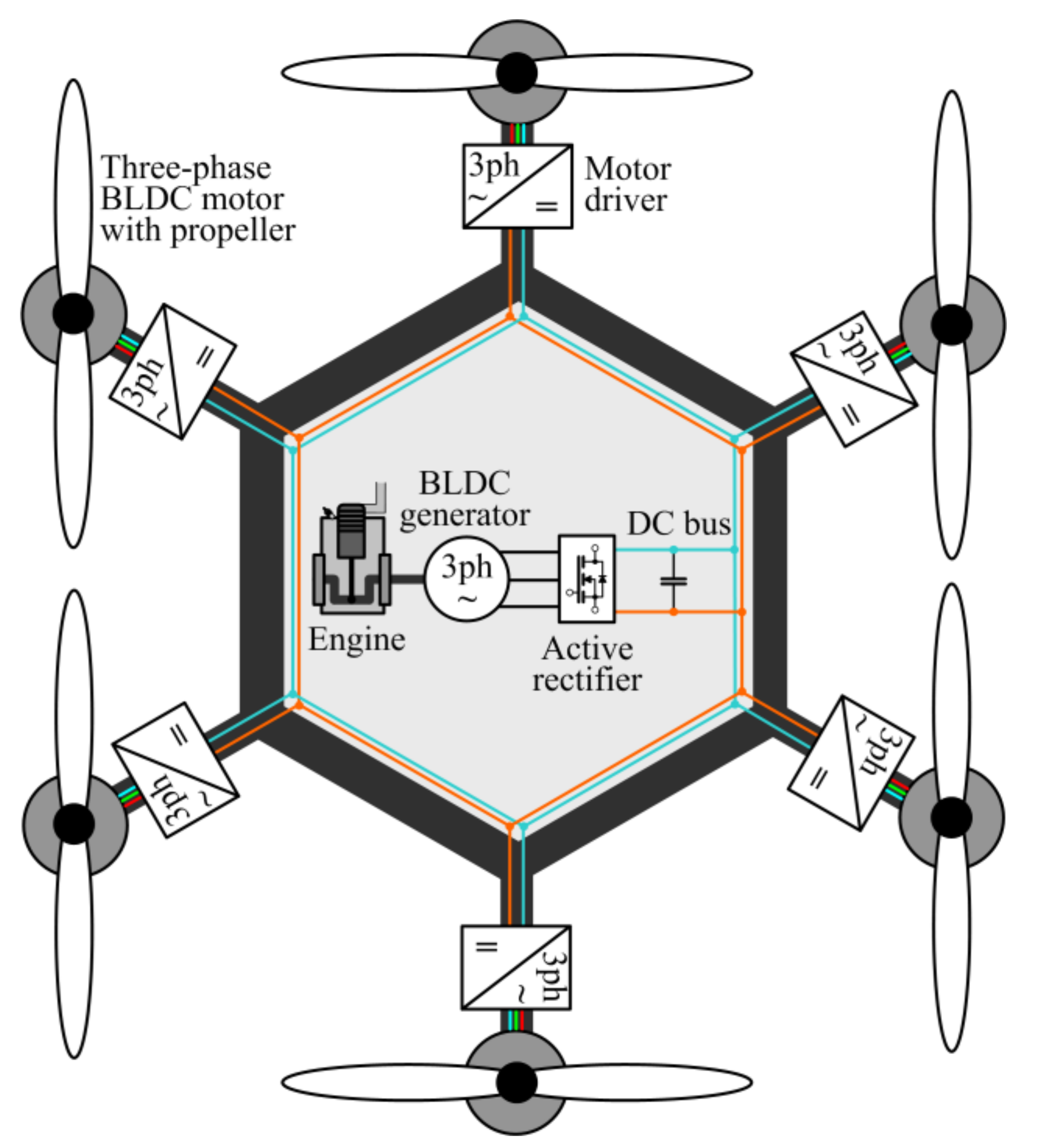
2.1. Hybrid Propulsion System Overview
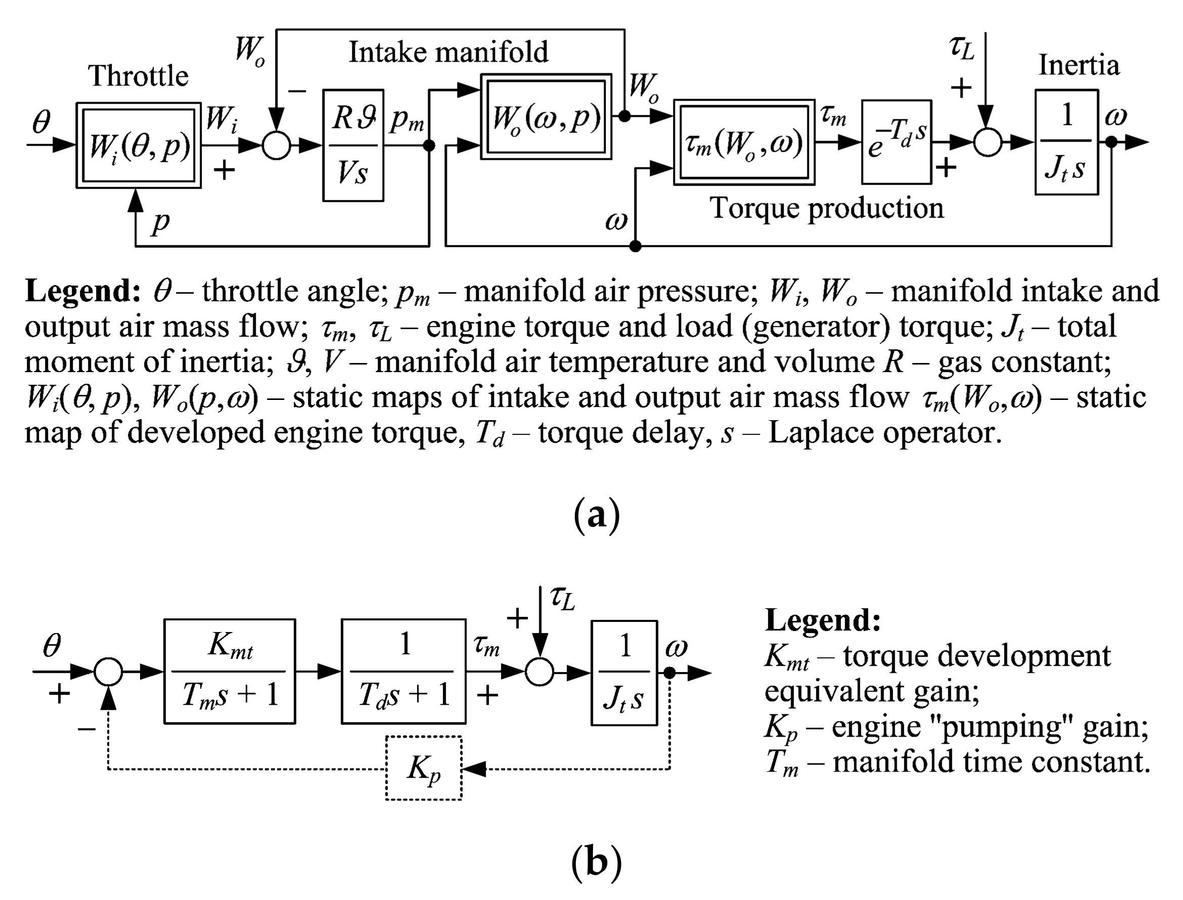
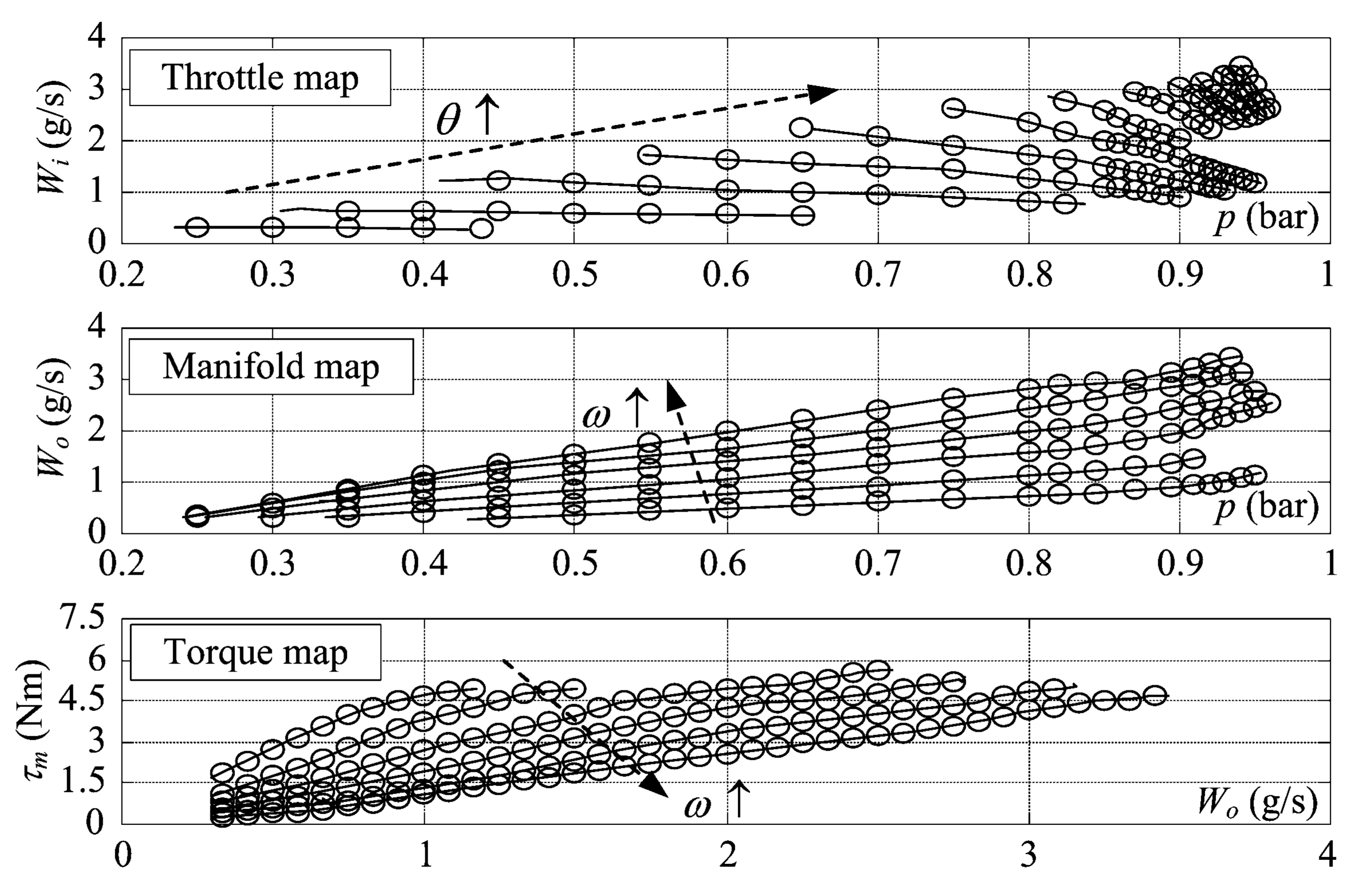
Figure 1 illustrates a possible realization of a hybrid propulsion-based UAV topology for the case of hypothetical hex-rotorcraft (comprising of six propeller drives). The on-board hybrid power system utilizes an internal combustion engine as the prime mover connected to the brushless DC generator, whose output power flow is controlled by an active rectifier (AC/DC power converter). Thus, the hybrid power system supplies the common DC bus in a controlled manner, i.e., DC bus voltage may be actively controlled via the power converter output power control.

2.2. Engine Model

Steady-state behavior and dynamics of the internal combustion engine (ICE) are typically modeled by means of mean value engine model (MVEM) [30], with isothermal heat transfer within the intake manifold. The nonlinear MVEM model (shown in Figure 2a) also comprises nonlinear static maps of the throttle servo-valve and the intake manifold, and the torque production map, along with the overall inertia at the engine side and the combustion event-related torque delay (i.e., dead time Td). The linearized ICE model suitable for control system analysis and design is shown in Figure 2b. This model, linearized in the vicinity of the engine operating point (τm, ω), is simpler in terms of throttle and manifold being described by the torque development equivalent gain and manifold time constant, while the torque delay is approximated by a first-order lag term with the time constant Td [31].

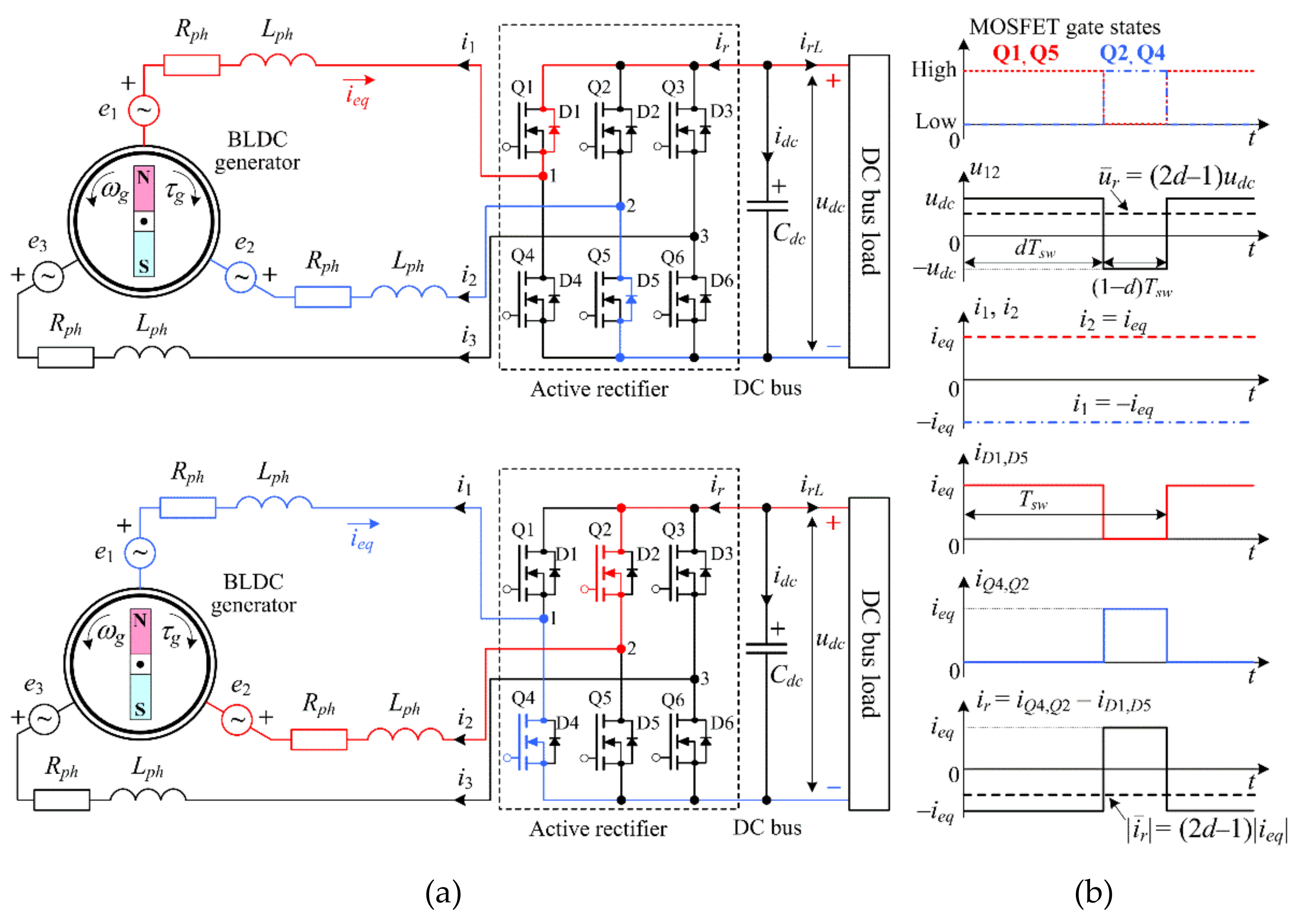
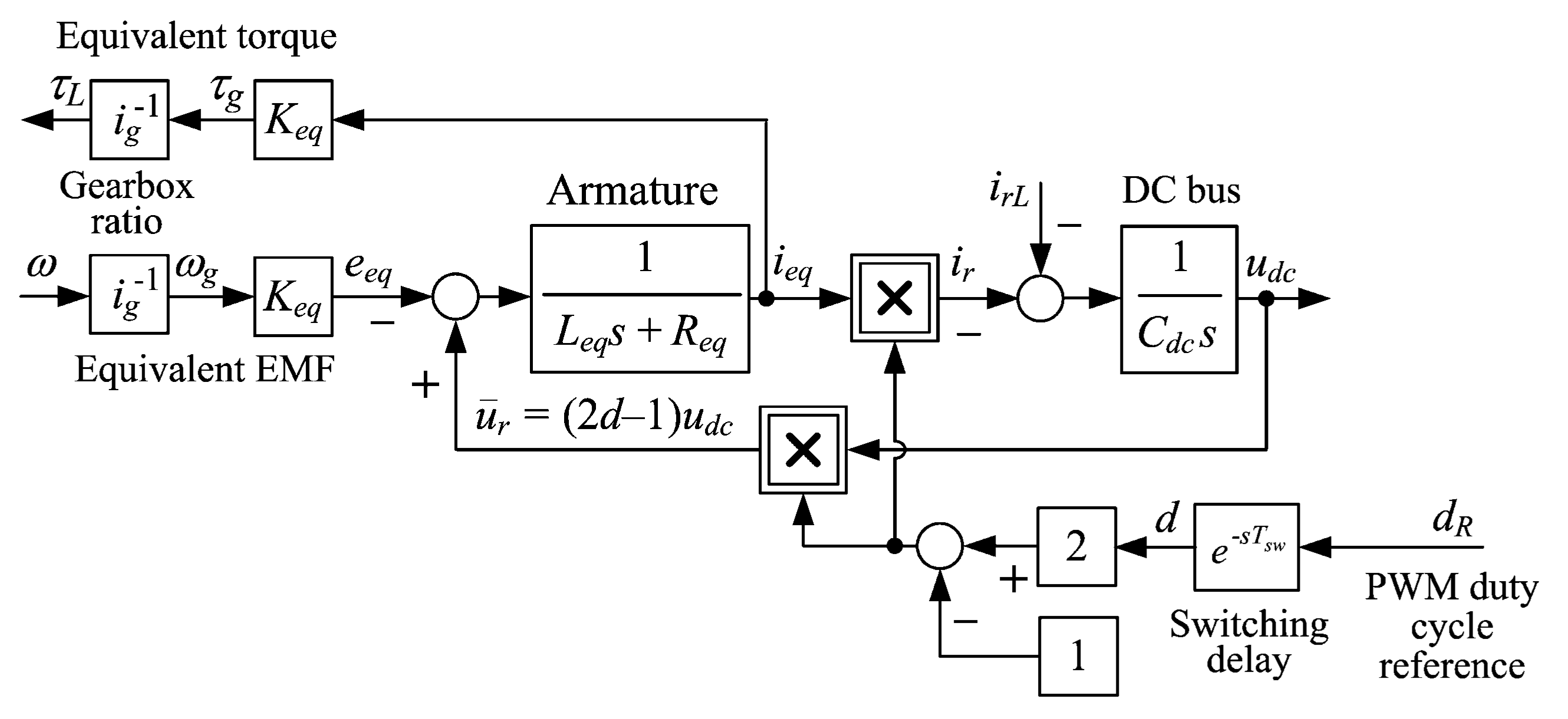
2.3. Brushless DC Generator with Active Rectifier-Supplied DC Bus

The principal schematic of the three-phase BLDC generator with rotor permanent magnets is shown in Figure 3a. Generator stator phase windings are characterized by equivalent internal resistance and inductance Rph and Lph, while the induced electromotive force (EMF) per each phase is given as follows [41]:
e l = K e ω g ϕ m p α g 2 π l 1 / 3 ,
where l = {1, 2, 3} represents the phase number and p is the number of pole pairs, ωg is the rotor rotational speed, φm is the rotor magnetic flux at stator side, which is dependent on the rotor position αg = ∫ωgdt (mechanical angle), and Ke is the EMF constant per phase.
On the other hand, the total electromagnetic torque of the brushless DC machine may be expressed in terms of individual phase currents il as follows:
τ g = K e l = 1 3 ϕ m p α g 2 π l 1 / 3 i l .
In contrast to the approach presented in [38], wherein a purely passive, diode-based three-phase full-wave rectifier is used to supply the DC bus, the DC bus voltage control herein is based on an active rectifier, i.e., fully-controlled DC/AC power converter equipped with dedicated MOSFET switches and freewheeling diodes, as shown in Figure 3a. Thus, DC bus voltage can be controlled via a pulse-width modulation (PWM) technique. More precisely, in each time instant, two stator phases are connected to the DC bus either through the MOSFET switches or through freewheeling diodes, depending on the pulse-width modulation (PWM) command applied to MOSFET switches gate inputs, with freewheeling diodes accounting for individual phase current flow continuity due to non-negligible inductance of stator phase windings [45]. During simultaneous conduction of two phases, the third phase is not powered. This is illustrated in Figure 3a corresponding to brushless DC machine supplying the DC bus (rectifier output current is negative, ir < 0). In particular, phases 1 and 2 are being energized and alternately connected to the DC bus voltage udc with positive or negative DC bus voltage sign, depending on the conditions for MOSFET power switch and freewheeling diode conduction. More precisely, the direction of the equivalent line current ieq needs to coincide with the current flow direction corresponding to conduction conditions of MOSFETs/diodes. For the scenario presented in Figure 3a, MOSFETs Q1 and Q5 are being triggered by appropriate gating signals during the time period (0, dTsw], but their conduction is not possible due to generator current having opposite (upwards) direction compared to MOSFET switch during conduction, so freewheeling diodes D1 and D5 conduct the generator equivalent line current ieq instead (Figure 3b). On the other hand, during the time period (dTsw, Tsw], the triggering signals energize the MOSFETs Q2 and Q4 and the equivalent line current ieq is able to flow through MOSFET switches [46]. This process is then repeated for different pairs of phases with respect to rotor electrical position, as shown in Table 1 (see, e.g., [41]).
Figure 3b shows the phase voltage waveforms for the case of PWM modulation of phase voltages and generator operation of the brushless DC machine. According to Figure 3a,b, i2 = –i1 = ieq is valid for the generator operating regime. Hence, the BLDC machine may be viewed as a DC machine during this particular time frame. The equivalent DC machine model armature circuit is characterized by the following values of equivalent inductances and resistances given [41]:
L e q = 2 L p h , R e q = 2 R p h + 2 r d ,
where double value of semiconductor component (MOSFET or diode) dynamic resistance rd is accounts for their respective conduction losses.
Using the same approach, and assuming the approximately rectangular rotor flux spatial distribution, the electromotive force and torque gains of the equivalent DC machine model take on values double the phase corresponding phase ones (Keq = 2Keϕmn). This results in the following algebraic equations for the equivalent EMF and torque values [41]:
e e q = K e q ω g = 2 K e ϕ m n ω g , τ g = K e q i e q = 2 K e ϕ m n i e q ,
where ieq is the instantaneous line (phase-to-phase) current (Figure 3a), and ϕmn is the constant-valued magnetic field flux of the rotor permanent magnets.
Note that the torque and EMF expressions given in Equation (4) are valid for the case of operation below the rated rotational speed, i.e., when rotor field flux weakening control is not applied, and which is assumed herein. If air gap field flux weakening is needed, it is typically carried out by means of armature voltage commutation angle (phase advance) variation with respect to EMF [47], which would result in values of EMF and torque constants that are lower than the nominal ones given in (4).
The equivalent line voltage ur (i.e., voltage across two stator phases) is obtained by pulse-width modulation (PWM) of the DC bus voltage with the suitably chosen switching frequency (fsw = 1/Tsw). Its average (mean) value can be expressed by using the DC bus voltage magnitude udc and the PWM duty cycle (0 ≤ d ≤ 1) as follows [46]:
u - r = 2 d 1 u d c .
Based on the above relationships, the BLDC machine stator winding model may be expressed in the following form in order to obtain the averaged armature model during simultaneous conduction of two phases:
L e q d i e q d t + R e q i e q = u - r e e q .
According to Figure 3b and analysis presented in [36], the brushless DC machine equivalent armature current (line current) ieq is related to the active rectifier current ir at the DC bus side as follows:
i r = 2 d 1 i e q .
Based on the above equivalent DC bus current formulation, the DC bus voltage dynamic equation is given as (Figure 3a):
u d c = 1 C d c i r + i r L d t ,
with irL being the DC bus load current (i.e., feeding the propeller drives and other loads).
The above relatively simple analysis yields the equivalent DC model of the brushless DC machine and active rectifier connected to the common DC bus shown in Figure 4, which is valid for operation below the rated speed. Apart from the armature (stator winding) phase-to-phase (line) resistance and inductance Req and Leq (calculated according to (3)), the model also includes the back electromotive force and developed mechanical torque of the equivalent DC machine model, which are calculated according to Equation (4). Thus, the mechanical part of the model (generator mechanical torque and rotational speed) can be easily integrated with the engine model in Figure 2 through the gearbox ratio ig, as shown in Figure 4.

3. Control System Design

Damping optimum-based control system design is presented in this section. A Luenberger estimator of generator rotational speed is used to provide feedback for the engine-generator set speed control system based on a proportional-integral-derivative (PID) feedback controller. Finally, DC bus voltage and current control system design is presented, based on respective proportional-integral (PI) feedback controllers.

3.1. Damping Optimum Criterion

Damping optimum criterion [44] is a pole-placement-type analytical method of design of linear continuous-time closed-loop systems, which can be quite useful when precise tuning of closed-loop damping is required. It has been successfully applied in power electronics systems control and electrical drive control applications (see, e.g., [48,49,50,51]).
The tuning procedure is based on the following closed-loop characteristic polynomial:
A s = D 2 n 1 D 3 n 2 D n T e n s n + + D 2 T e 2 s 2 + T e s + 1 ,
with Te being the closed-loop system equivalent time constant, and D2, D3,…, Dn being the so-called damping optimum characteristic ratios.
In the so-called “optimal” case Di = 0.5 (i = 2 … n), the closed-loop system step response (for any closed-loop system order n) is characterized by an overshoot of approximately 6% (thus emulating a second-order system behavior with the damping ratio ζ = 0.707) with the approximate step response rise time tr = 2·Te. In general, larger Te values correspond to improved control system robustness and noise suppression ability, albeit with slower closed-loop response, and vice versa.
From the standpoint of designing of a superimposed controller, the inner closed-loop system tuned according to the damping optimum criterion may be approximated by the equivalent first-order lag transfer function characterized by the closed-loop equivalent time constant Te (under assumption of unit gain of the inner closed loop model):
G e s = 1 T e s + 1 .

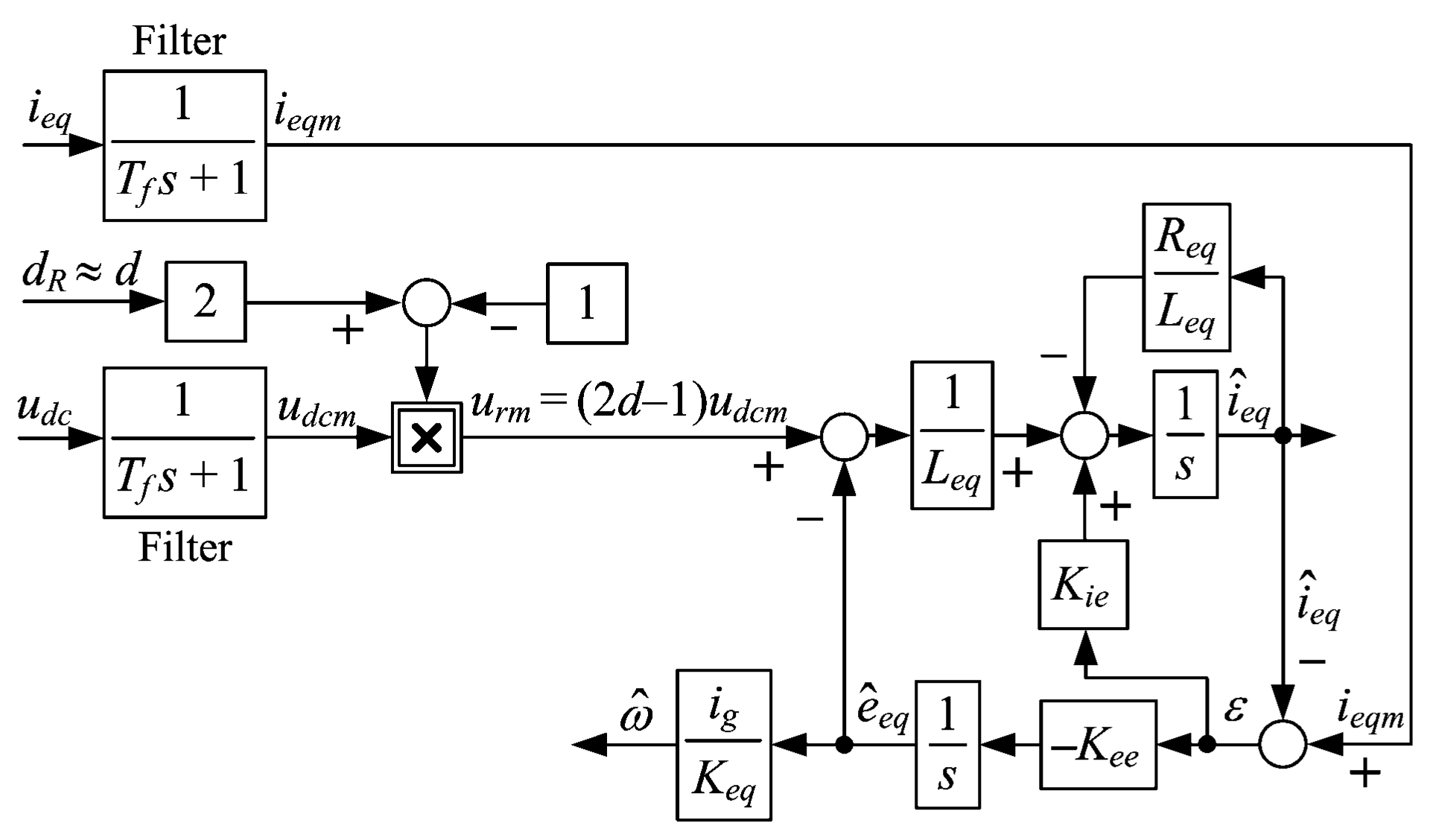
3.2. Engine-Generator Set Rotational Speed Estimator

Even though low-resolution position measurement of a BLDC machine or permanent-magnet synchronous machine (PMSM) based on Hall sensors can be quite robust and may sometimes replace the resolver or encoder-based position measurements [52], such an approach typically indicates electrical angle change of 60 degrees when rotor magnets travel between two stator phases [52]. According to the analysis presented in [42], this may result in pronounced speed measurement noise due to quantized position signal differentiation, with such speed measurement also being characterized by a perceptible delay at low speeds due to relatively large sampling time needed as well as filtering of thus obtained speed signal to attenuate the quantization noise. On the other hand, the study in [42] has also indicated that position-sensorless approach, relying on back-electromotive force estimation may result in superior engine-generator set speed tracking ability in terms of response speed and measurement noise levels. Thus, the back electromotive force estimation approach is also used herein for engine-generator set speed control.
Brushless DC machine equivalent DC model in Equation (6) is used for speed estimation, with the armature EMF eeq = Keqω/ig variable treated as the unknown disturbance and modeled by a first-order disturbance model. The resulting Luenberger estimator [43] of the engine-generator set rotary speed utilizes equivalent DC current (i.e., line current) and DC bus voltage measurements ieqm and udcm obtained from corresponding sensors characterized by the equivalent low-pass filtering dynamics given by (see block diagram in Figure 5):
G f s = 1 T f s + 1 ,
with Tf being the current/voltage signal filter equivalent time constant.
Based on the known (and readily available) PWM switching command duty cycle reference dR, the active rectifier output voltage estimate urm can be reconstructed based on equation (5) and used as estimator input, thus finally yielding the following Luenberger estimator state-space formulation (Figure 5):
d ı ^ e q / d t d e ^ e q / d t = R e q / L e q 1 / L e q 0 0 ı ^ e q e ^ e q + 1 / L e q 0 u r m + K e i K e e ı e q m ı ^ e q ,
The above state-space estimator representation can be transformed into its Laplacé s-domain transfer function counterpart as follows:
ω ^ s = i g K e q u r m s L e q s + R e q i e q m s A o s ,
with the estimator transfer function characteristic polynomial Ao(s) given as:
A o s = s 2 L e q K e e + s R e q K e e + L e q K i e K e e + 1 .
Thus, the above estimator model outputs a scaled and low-pass filtered value of the “raw” reconstruction of the equivalent electromotive force (EMF) according to equation (6), i.e., eeq = urLeqdieq/dtReqieq, which is additionally filtered by the voltage/current measurement filters with the time constant Tf (Figure 5).
Luenberger estimator is designed by equating the above low-pass filter transfer function denominator with the second order damping optimum characteristic polynomial according to Equation (9), which yields the following results for Luenberger estimator gains Kee and Kie:
K e e = L e q D 2 o T e o 2 , K i e = 1 D 2 o T e o R e q L e q ,
with the following feasibility condition imposed upon the equivalent time constant Teo:
T e o < 1 D 2 o L e q R e q .

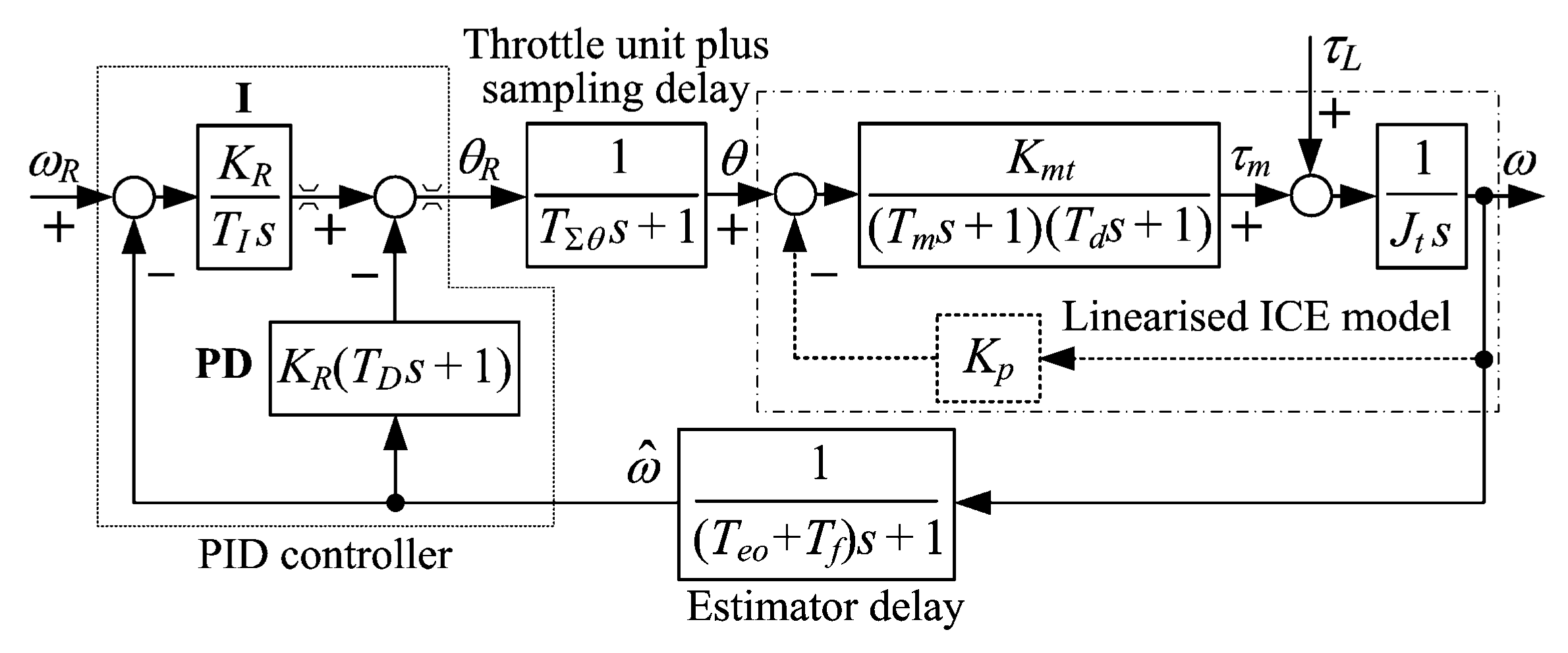
3.3. Engine Speed Control System

The block diagram representation of the linearized engine speed control system featuring a PID feedback controller is shown in Figure 6. The parameters of the linearized ICE model (Figure 2b) are obtained according to the procedure presented in [41], and their values used in subsequent analyses are given in Section 5. The engine speed controller commands the throttle valve position target value θR to the throttle valve servodrive, whose dynamics are approximated by a first-order lag term with time constant TΣθ. The aforementioned time delay may also include the controller sampling lag [34].
Based on the linearized ICE speed control system representation in Figure 6, PID controller design according to the damping optimum criterion yields the following expressions for the controller parameters (i.e., equivalent time constant T, gain KR, and integral and derivative time constants TI and TD) [48]:
T e ω T e ω m i n = 1 D 2 ω D 3 ω D 4 ω T Σ θ + T e o + T f T d + T m + T d T m T Σ θ + T e o + T f + T d + T m ,
K R = J t D 2 ω 2 D 3 ω T e ω 2 T Σ θ + T e o + T f + T d + T m K m t K p ,
T I = T e ω 1 + K p K R 1 ,
T D = J t K m t K R T Σ θ + T e o + T f + T d + T m D 2 ω D 3 ω T e ω 1 T Σ θ + T e o + T f K p K R ,

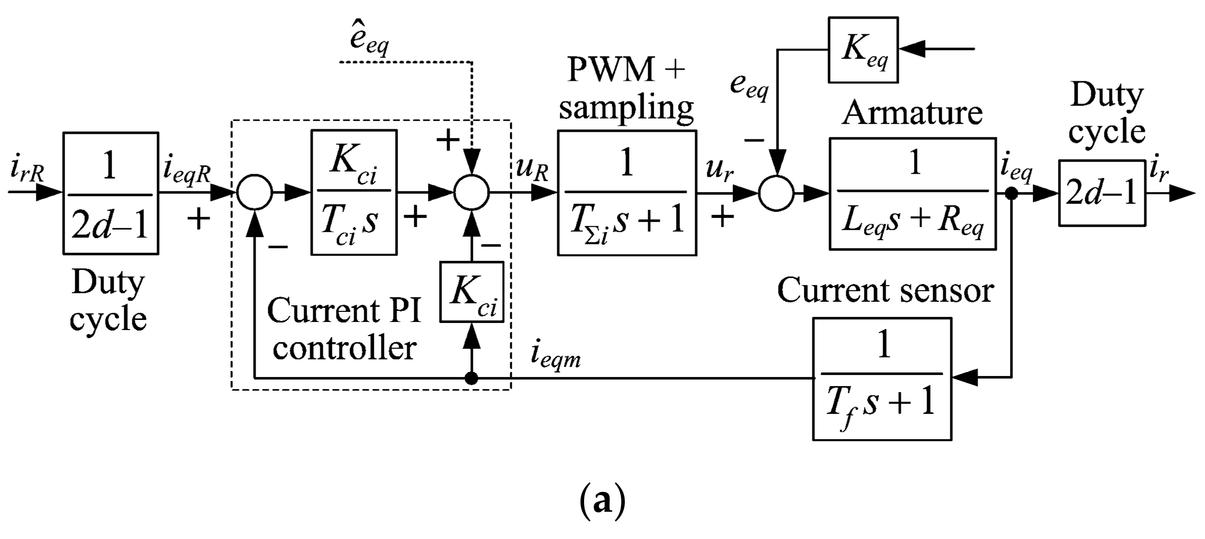
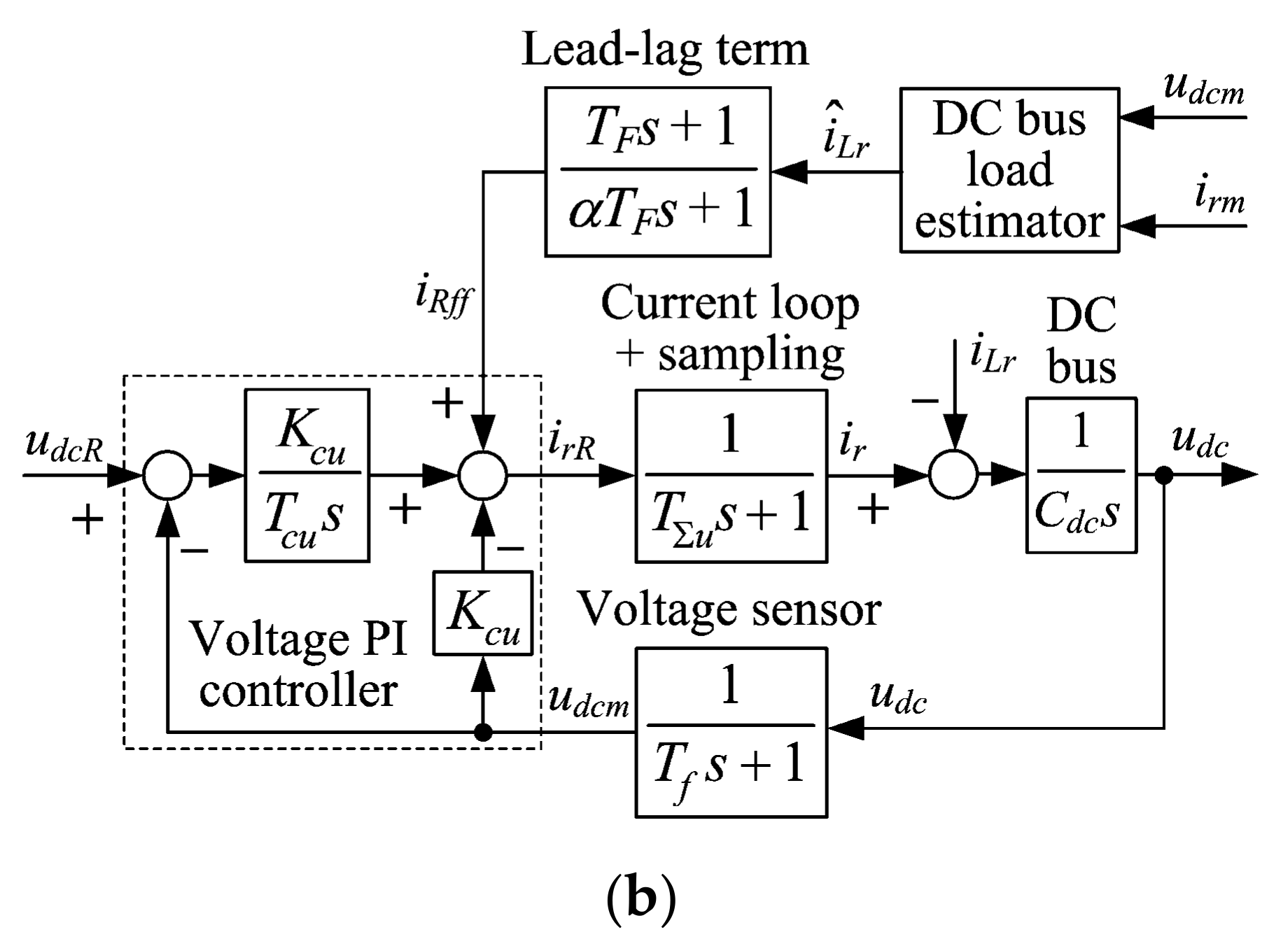
3.4. DC Bus Voltage and Current Control Systems

Brushless DC machine line current and DC bus voltage feedback control loops are shown in Figure 7a,b, respectively. Both feedback loops include proportional-integral (PI) feedback controllers, which are augmented by feed-forward load compensators based on suitable estimators of local disturbance variables (back electromotive force in the case of current control loop, and load current in the case of DC bus voltage control loop). The parameters of the generator armature voltage vs. current model are obtained experimentally in [53], while the DC bus capacitance and measurement filter lag Tf used herein are chosen based on a similar study conducted in [49]. These values, used in subsequent simulation analyses, are given in Section 5.
The electromotive force (EMF) “disturbance” within the current control loop can be dealt with by using the readily available EMF estimate from the engine-generator speed estimator (see Section 3.2), whereas in the case of DC bus load, a Luenberger state estimator can be used to reconstruct the load current irL from the available measurements of active rectifier current irm and DC bus voltage udcm:
d u ^ d c / d t d ı ^ r L / d t = 0 1 / C d c 0 0 u ^ d c ı ^ r L + 1 / C d c 0 i r m + K d c e K L e u d c m u ^ d c .
Again, the above Luenberger estimator can be represented by its transfer function model, and the resulting DC bus load estimate vs. estimator inputs model has the form of low-pass filtered “raw” reconstruction of load current irL = –(ir + Cdcdudc/dt) according to the DC bus model in Equation (8):
ı ^ r L s = i r m s + C d c s u d c m s A L s = i r m s + C d c s u d c m s s 2 C d c K L e + s C d c K d c e K L e + 1 .
Damping optimum criterion yields the final expressions between the DC bus load estimator gains, DC bus capacitance Cdc and damping optimum parameters (characteristic ratio D2L and equivalent time constant TeL):
K L e = C d c D 2 L T e L 2 , K d c e = 1 D 2 L T e L .
In the BLDC armature current control loop design, the rather small PWM switching delay and controller sampling delay (if digital controller is considered) are lumped into the parasitic time constant TΣi (Figure 7a). This lag is augmented by the current sensor lag Tf in order to obtain the so-called “lumped” first-order lag term with the equivalent time constant Tpi = TΣi + Tf which approximates the fast closed-loop dynamics. Using this approximation, the following closed-loop transfer function model (similar to the case presented in [50]) is obtained, and used in BLDC machine current control system design:
G c i s = i r s i r R s = 1 T p i L e q T c i s 3 K c i + R e q T p i + L e q T c i s 2 K c i + R e q + K c i T c i s K c i + 1 .
By applying the damping optimum criterion, the following results for current controller parameters are obtained:
T e i T e i , m i n = 1 D 2 i D 3 i T p i 1 + T p i R e q / L e q ,
T c i = T e i 1 D 2 i T e i T p i + L e q / R e q ,
K c i = R e q T p i + L e q / R e q D 2 i T e i 1 .
Note that according to Equation (7), the current reference (target value) irR needs to be adjusted with respect to the actual PWM duty cycle value to command a proper line current reference ieqR (input scaling block in block diagram in Figure 7a). The power converter duty cycle target value d is in fact commanded by the current control loop through line voltage reference value uR, so it is readily available using Equation (5). However, it should also be averaged to avoid noise issues, along with avoiding division by zero issues at zero mean voltages (d = 0.5) [49].
Similar to the above control system design procedure, in the DC bus voltage PI feedback controller design the parasitic time constant TΣu includes the current control loop equivalent time constant Tei and the controller sampling time T (if digital controller is used). This results in the overall first-order lag term with the time constant Tpu = TΣu + Tf describing the “fast” voltage control loop dynamics, and the corresponding closed-loop system transfer function model is given as follows:
G u d c s = u d c m s u d c R s = 1 C d c T Σ u + T f T c u K c u s 3 + C d c T c u K c u s 2 + T c u s + 1 .
By applying the damping optimum criterion, the following expressions for DC bus voltage PI controller parameters are obtained (see, e.g., [49]):
T c u = T e u = T Σ u + T f D 2 u D 3 u ,
K c u = C d c D 2 u T e u .
Finally, the feed-forward compensator (lead-lag filter) is designed with the aim of canceling out the main dynamics of the inner current control loop (i.e., its equivalent lag Tei). The zero-pole canceling approach yields the so-called “lead” time constant TF = Tei with the filtering pole sF = 1/(αTF) scaling factor α typically chosen in the range α = 0.1 … 0.6.

4. Control System Robustness Analysis

In order to investigate the effect of key process parameters variations to control system behavior, robustness analysis to armature voltage and current measurement errors and armature resistance variations is carried out for the brushless DC generator electromotive force (EMF)/engine speed estimator and generator current/DC bus voltage control system. Finally, the engine speed control system robustness is analyzed for the case of torque gain and manifold time constant variations with respect to actual values.

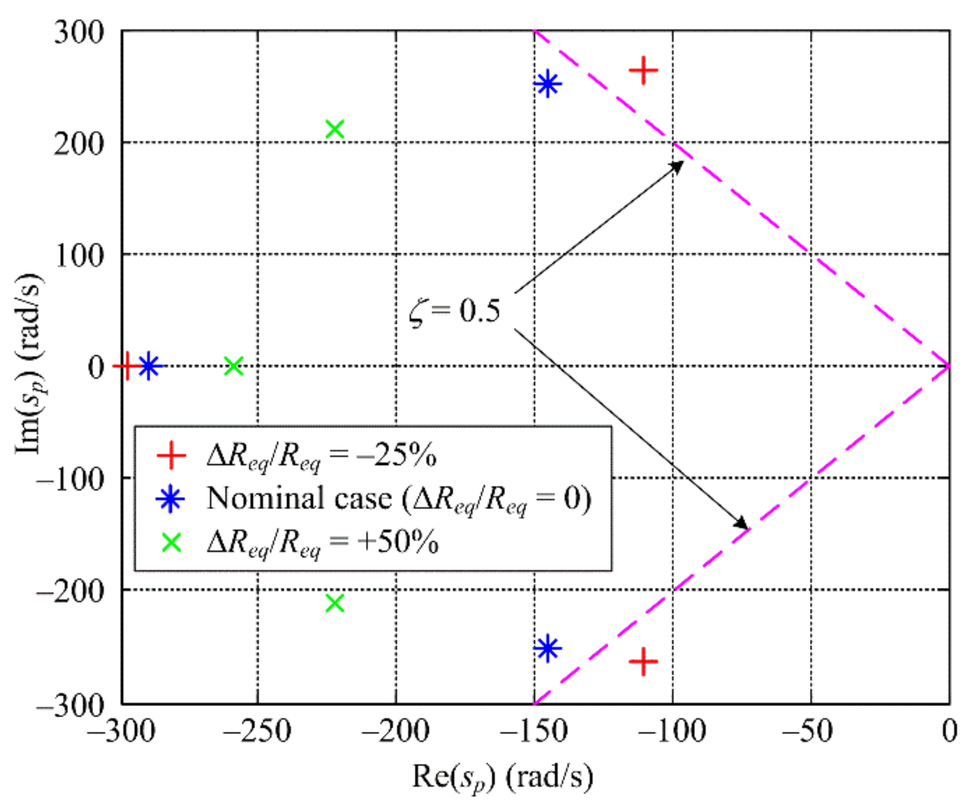
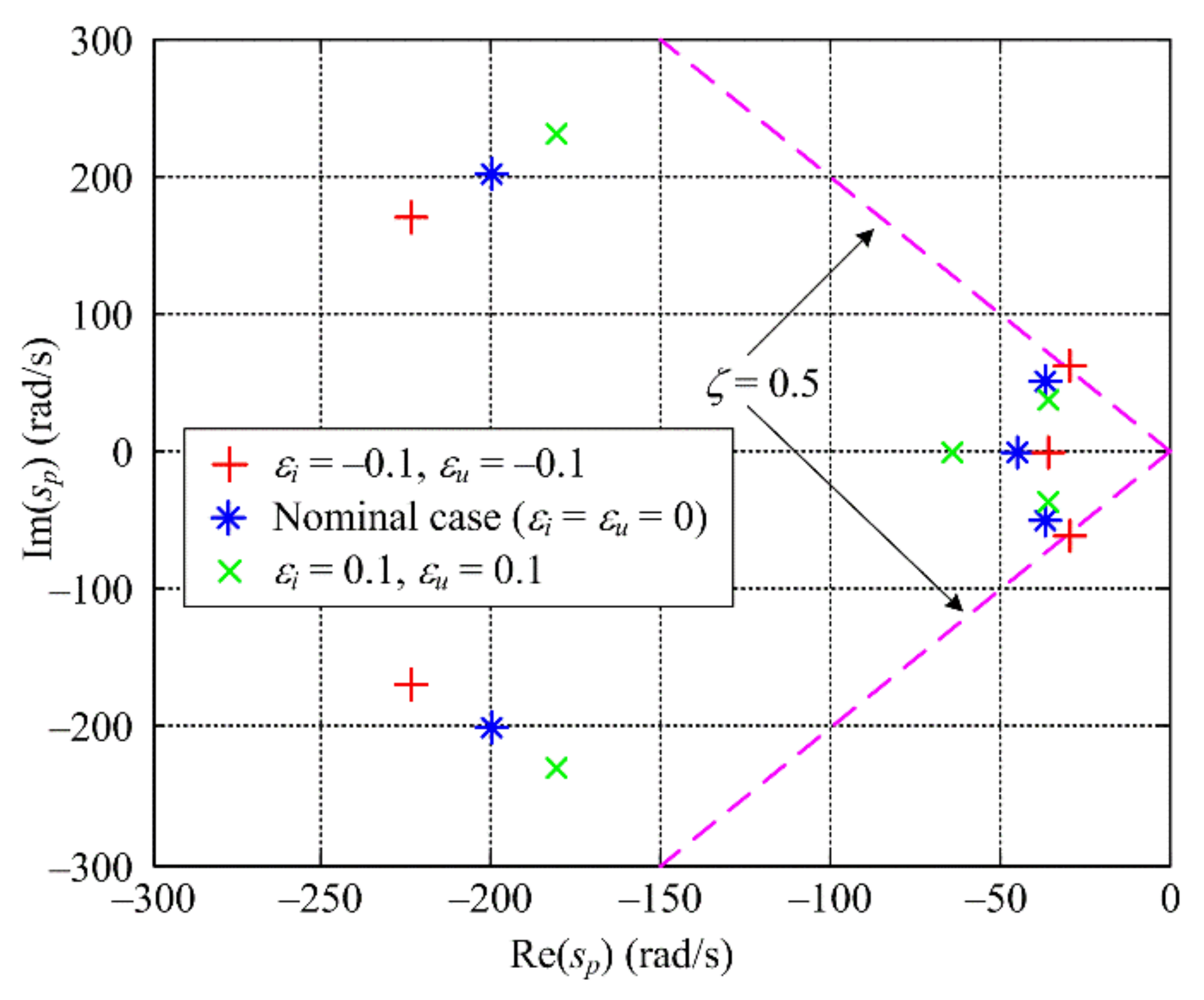
4.1. Generator Current Control System Robustness to Armature Resistance Variations

In the generator closed-loop control system robustness analysis variations of the equivalent armature resistance Req (e.g., due to armature winding temperature variations) can be modeled as constant-valued offset error ΔReq with respect to the nominal resistance value Req which is used in the closed-loop control system design (see Equations (24)–(27)):
R e q * = R e q + Δ R e q .
After the aforementioned modeling error is included within the closed-loop transfer function model (24), the closed-loop characteristic polynomial reads as follows:
A c i s = T p i L e q T c i s 3 K c i + R e q * T p i + L e q T c i s 2 K c i + R e q * + K c i T c i s K c i + 1 .
which can be used to illustrate the armature resistance variation effects to the closed-loop damping (and stability) by means of root-locus plots.
The resulting root locus plots for the relative armature resistance variations ΔReq/Req from −25% to +50% are shown in Figure 8, with these boundary cases represents a realistic scenario in practical applications, as indicated in [48]. As indicated by closed-loop pole locations in Figure 8, if armature resistance is increased above the nominal value, this results in increased closed-loop damping, whereas armature resistance decrease may result in decreased closed-loop damping. The latter scenario is usually related to ambient temperature decrease and would typically have less effect during brushless DC generator operation due to unavoidable machine internal heat losses. Thus, it may be surmised that favorable closed-loop damping of BLDC generator armature current control system should be maintained for the particular realistic range of armature resistance variations.

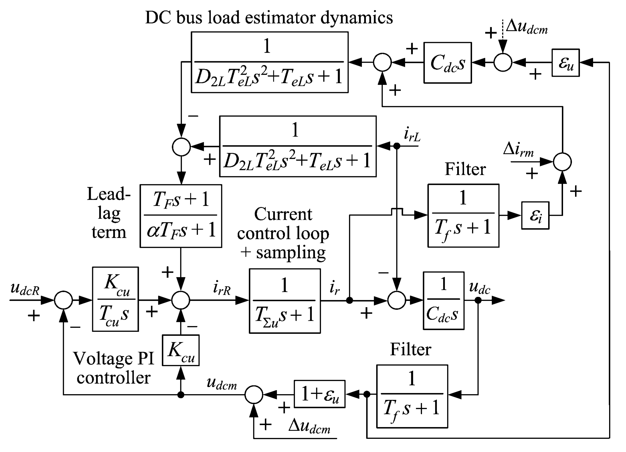
4.2. DC Bus Voltage Control System Robustness to Sensor Errors

The DC bus voltage control loop, comprising the voltage PI controller and load compensator based on Luenberger estimator may be sensitive to errors of DC bus voltage measurement udcm and DC bus current reconstruction irm, both used within the load estimator. The voltage/current sensor errors may generally be modeled as gain plus offset errors [49]:
u d c m = 1 + ε u u d c + Δ u d c m ,
i r m = 1 + ε i i r + Δ i r m ,
where εu and εi are gain (multiplicative) voltage reconstruction and current measurement errors, while Δurm and Δieqm are the corresponding constant-valued voltage and current offset errors.
The above relationships (33) and (34) are taken into account within the overall DC bus voltage control system model (Figure 7) and the Luenberger estimator-based load compensator (Equation (12)), so that the DC bus control system closed-loop model may be represented by the block diagram shown in Figure 9. The DC bus controller and estimator parameters are obtained according to the design procedure in Section 3, while the process model parameters (DC bus capacitance and filter lag) are chosen as explained in previous section. For the purpose of simplicity, the Luenberger estimator dynamics are characterized herein by the estimator characteristic polynomial AL(s) (22) rewritten in terms of 2nd-order damping optimum characteristic polynomial (Figure 9):
A L s = D 2 L T e L 2 s 2 + T e L s + 1 .
As shown in [49], the feed-forward load compensator action subject to current and voltage sensor gain errors according to Equations (33) and (34) can be divided into the “nominal” feed-forward action and the “parasitic” sensor error-related dynamics. The latter may be considered as additional virtual feedback paths of current ir and voltage udc signals (see Figure 9) which may affect the closed-loop robustness (i.e., damping) [49]. Voltage offset and gain errors may also result in steady-state control error, while the current offset error (Δirm) would be suppressed by the integral action of the DC bus voltage PI controller.
Root locus plots of the DC bus voltage closed-loop control system subject to voltage/current sensor gain errors are shown in Figure 10. The case of ±10% gain errors is considered herein as a worst-case scenario, as suggested in [49]. As expected, the closed-loop pole locations are shifted from the nominal positions (corresponding to zero sensor gain errors), with dominant pole locations being characterized by less well-damped closed-loop pole locations for the case of negative gain errors (εi = εu = −0.1). The less dominant closed-loop poles behave in an opposite manner, i.e., they are shifted towards less well-damped locations (i.e., towards the origin of the s-plane) in the case of positive sensor gain errors (εi = εu = +0.1), but they remain well-damped for the considered hypothetical range of sensor gain errors.

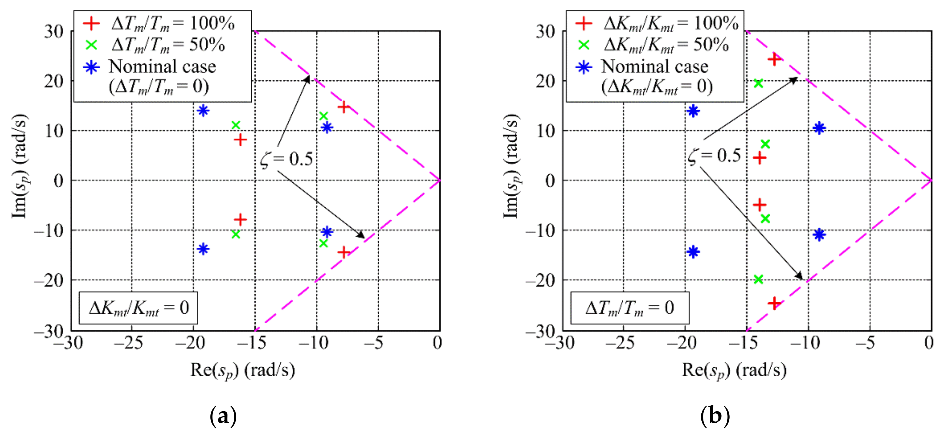
4.3. Engine Speed Control System Robustness to Torque Gain and Manifold Lag Errors

It is assumed that the engine torque gain Kmt and manifold time constant (lag) Tm of the linearized engine model (Figure 2b) are subject to additive errors ΔKmt and ΔTm, thus resulting in the following torque gain and time constant K*mt and T*m values:
K m t * = K m t + Δ K m t ,
T m * = T m + Δ T m ,
while the total inertia Jt and throttle lag Tθ are assumed constant (which is a realistic assumption during engine-generator set operation), while the torque development lag (dead-time) Td can be calculated in real time based on engine speed information, as indicated in [30,31].
In that case, the closed-loop dynamics of the linearized engine speed control system (Figure 6) with respect to speed target are modeled as follows [48]:
G c s = ω s ω R s = 1 A c s = 1 1 + a ω 1 s + a ω 2 s 2 + a ω 3 s 3 + a ω 4 s 4 + a ω 5 s 5 ,
where:
a ω 1 = 1 + K p K R T I ,
a ω 2 = J t + K m t * K R T D + K p T Σ θ + T f + T e o K m t * K R T I ,
a ω 3 = T Σ θ + T f + T e o + T m * + T d K m t * K R J t T I ,
a ω 4 = T Σ θ + T f + T e o T m * + T d + T m * T d K m t * K R J t T I ω ,
a ω 5 = T Σ θ + T f + T e o T m * T d K m t * K R J t T I .
Based on the above closed-loop system model, Figure 11 shows the closed-loop pole locations for the torque gain Kmt and time constant Tm relative errors of 50% and 100%. The root locus analysis results are obtained for engine speed PID controller tuned with T = Tmin (Equation (17)), which relates to a fast and well-damped response of the engine speed control loop. The results in Figure 11a show that the intake manifold time constant error causes the dominant conjugate-complex pole pair to be shifted towards the origin of the s-plane. A similar result is also obtained for linearized engine model torque gain parameter variation (Figure 11b), with the dominant conjugate-complex poles being characterized by decreased damping and larger imaginary parts. However, in both cases the closed-loop pole damping ratio is kept above ζ = 0.5, which points out to rather favorable robustness of the proposed tuning approach.

4.4. Luenberger Estimator-Based Speed Estimation Accuracy

According to Figure 5, the engine-generator set speed estimation based on BLDC machine armature measurements and Luenberger estimator methodology may be sensitive to error of armature voltage urm reconstruction and equivalent armature current ieqm measurement, along with the mismatch of the actual armature resistance and its nominal value used in Equation (6). Again, the armature voltage/current measurement errors can be modeled as gain plus offset errors:
u r m = 1 + ε u u - r + Δ u r m ,
i e q m = 1 + ε i i e q + Δ i e q m ,
where εu and εi are respective gain (multiplicative) voltage reconstruction and current measurement errors, while Δurm and Δieqm are the corresponding constant-valued voltage and current offset errors.
If the aforementioned relationships Equations (31), (44) and (45) are taken into account within the overall Luenberger estimator model (Equation (13)), the following dynamic model of generator speed estimation is obtained after some manipulation and rearranging (cf. also Figure 5):
ω ^ s = ω s + Δ ω s + ω o f f A o s T f s + 1 ,
where the constant-valued speed measurement (estimation) offset ωoff and speed estimation dynamic error Δω(s) are given as follows:
ω o f f = i g K e q Δ u r m R e q + Δ R e q Δ i e q ,
Δ ω s = i g K e q ε u u - r s L e q s + R e q ε i i e q m s Δ R e q 1 + ε i i e q m s .
Obviously, the pure offset ωoff of engine-generator set speed estimation is caused by armature current and voltage measurement offset errors and armature resistance variations, ultimately resulting in engine-generator set closed-loop steady-state error. On the other hand, the speed estimation error component Δω(s) due to voltage/current measurement gain errors may affect the engine speed control system closed-loop performance during transients and in the engine generator set steady-state. These speed estimation errors are examined in more detail by means of simulations in the next section.

5. Simulation results

5.1. Simulation Model Parameterization

The proposed control systems for the presented hybrid power supply are verified by means of simulations carried out in MATLAB/Simulink. Simulation models are parameterized based on data from [31,34,53,54,55,56], with final parameters of linearized process models listed in Table 2. MVEM model maps used for ICE simulation are obtained by re-scaling the engine maps from [31,34] using the methodology proposed in [57], and these maps are shown in Figure 12. The values of parameters of individual controllers and estimators presented in this work and used throughout the simulation study are also listed in Table 2.

5.2. Results of Simulation Analyses

Figure 13 shows the comprehensive simulation results of the overall speed-controlled engine-generator set equipped with active rectifier supplying the DC bus under the voltage/current control scheme and featuring Luenberger estimators of engine-generator set rotational speed and DC bus load for the nominal case (no process/plant parameter variations). Figure 13a shows the responses of the engine speed control system with PID speed feedback controller utilizing the engine speed estimate. Top plot in Figure 13a shows the engine speed responses to a sudden generator load change of 10 A (see middle plot in Figure 13b)), which corresponds to a 1.25 Nm load change at the engine side (approximately 20% of the engine maximum torque according to torque map in Figure 12). The engine speed response under PID control is characterized by a well-damped transient and favorable suppression of abrupt load disturbance. In particular, engine speed recovery is achieved within 0.6 s after the load change, and the closed-loop response is characterized by a relatively non-emphasized 700 rpm speed drop (15.6% of the engine target speed value ωR = 4500 rpm). The well-damped behavior of the closed-loop engine speed control system is also evident in the engine torque and throttle responses (middle and bottom plots in Figure 13a), which are characterized by initial abrupt change after the load disturbance, and smooth control action (throttle reference θR) commanded during the closed-loop response settling phase. Figure 13b shows the active rectifier-based DC bus control system responses during the DC bus load change, wherein the voltage/current control system exhibits a relatively modest DC bus voltage drop (top plot in Figure 13b) of 5 V. This corresponds to 10.4% of the DC bus voltage target value after the sudden load change, with the recovery time of 80 ms and response settling time of 200 ms. Such an effective load suppression action is achieved by utilizing the fast feed-forward compensator based on the estimated DC bus load (middle plot in Figure 13b) within the voltage control loop (cf. Figure 7b). The shape of the electromotive force estimate (bottom plot in Figure 13b) closely matches the shape of the engine-generator speed trace (top plot in Figure 13a).
Simulation results of the engine-generator set speed control system for the case of brushless DC generator armature resistance mismatch and armature current and voltage measurement (sensor) errors are shown in Figure 14. These results cover the worst-case scenarios in terms of closed-loop system robustness analyzed in the previous section (i.e., ±10% voltage/current sensor gain errors εu and εi and -armature resistance variation from the nominal value ΔReq/Req = 25% are considered), along with relatively small current/voltage measurement offset errors (Δurm = 0.2 V, and Δirm = 0.2 A) The results in Figure 14 point out that the anticipated range of process model parameter variations introduces notable steady-state engine control error, whereas negative speed offset is obtained for positive sensor gain errors (Figure 14a), while positive speed offset is associated with negative gain error values (Figure 14b). Since only positive voltage/current offset errors are introduced in the simulation, their effect is visible in the magnitude of the actual engine-generator set speed offset from the target value, wherein larger speed control errors are obtained for the same sign of sensor gain and offset error, and vice versa (cf. top plots in Figure 14a,b). The effect of voltage/current sensor gain error is also manifested in the closed-loop system speed transient damping after a sudden load torque change, wherein positive gain errors (εu = εi = 0.1) decrease the level of closed-loop damping, which is characterized by somewhat larger load response overshoot compared to the nominal case (cf. middle and bottom plots of developed engine torque and throttle command in Figure 13a and Figure 14a), whereas negative gain errors (εu = εi = −0.1) tend to increase the level of closed-loop damping (cf. Figure 13a and Figure 14b).
Figure 15 shows the results of DC bus control system simulations subject to DC bus voltage and active rectifier current sensor gain and offset errors. As predicted by the robustness analysis in the previous section, voltage offset and gain errors result in steady state DC bus control error (cf. top plots in Figure 15a,b). Again, larger control error absolute values are obtained for the same sign of sensor gain and offset error, and vice versa. Moreover, the current and voltage reconstruction errors may also affect the steady-state accuracy of the load current estimation based on Luenberger estimator, as shown in bottom plots in Figure 15a,b. However, due to integral action of the DC bus PI controller, the active rectifier current is correctly commanded in order to maintain the steady-state DC bus voltage (nonetheless being affected by the accuracy of DC bus voltage measurement). The effects of sensor gain errors to closed-loop damping match the findings of the closed-loop system robustness analysis, wherein closed-loop damping level is decreased for negative sensor gain errors (εi = εu = −0.1) compared to nominal case (cf. top plots in Figure 13b and Figure 15a), as opposed to the case of positive sensor gain errors (εi = εu = 0.1), see top plot in Figure 15b.

6. Discussion of Results

Robustness analysis of the overall control system to parameters variations within process models (i.e., parameters of the controlled hybrid power-plant) has yielded the following findings:
(i)
Brushless DC machine armature current control system should be fairly robust to armature resistance variations over the expected range of its variations;
(ii)
DC bus control system sensitivity to voltage and current sensor gain and offset error may manifest in closed-loop voltage control error, with possibly decreased level of damping of the dominant closed-loop poles in the case of negative sensor gain errors;
(iii)
The engine-generator set speed control system should be robust to a relatively large change of manifold lag and equivalent engine torque gain parameter.
(iv)
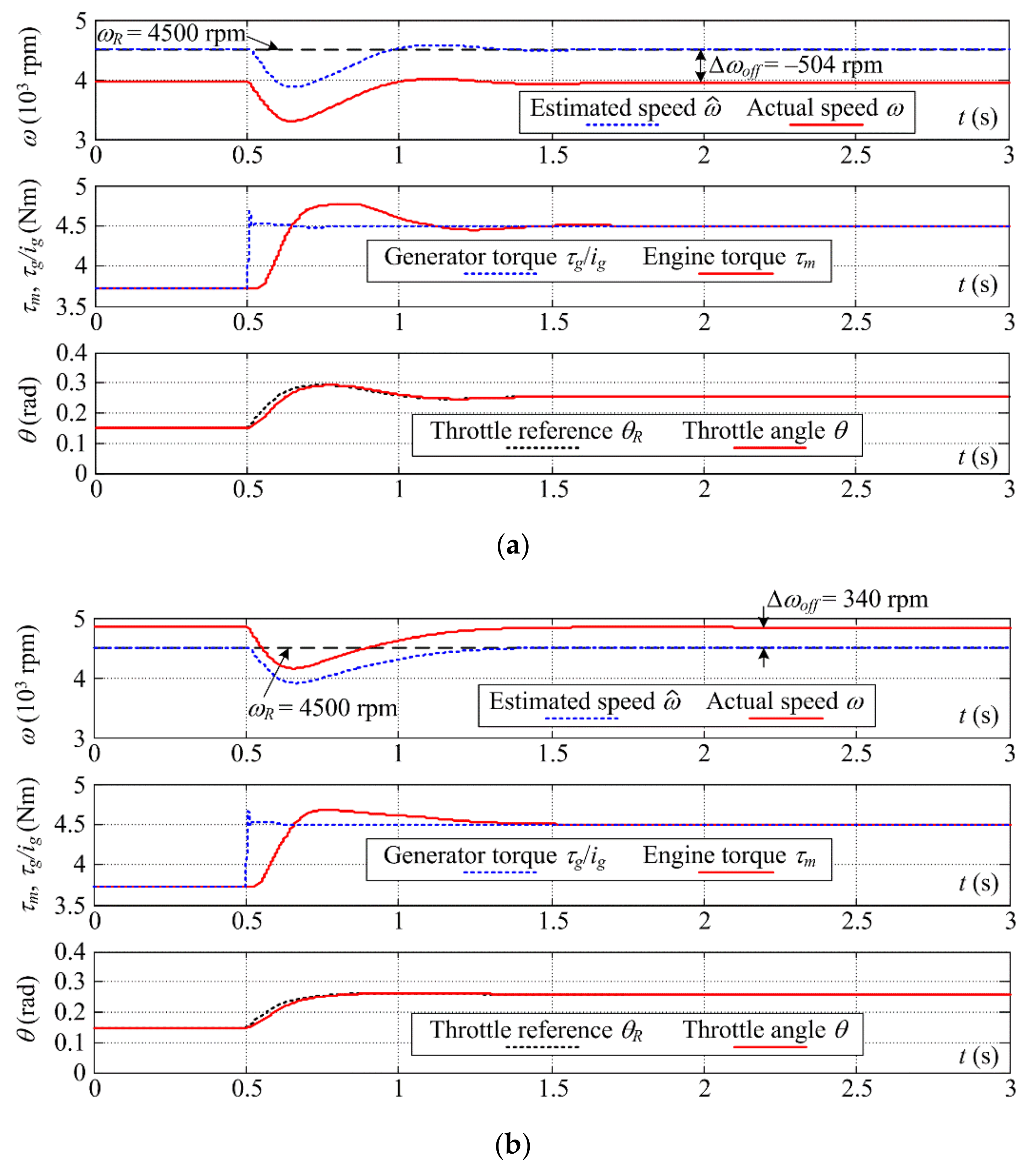
The generator current and voltage sensor errors may affect both the steady-state and transient accuracy of the engine-generator speed estimation. The steady-state estimation error is solely affected by the current/voltage sensor offset errors and generator armature resistance mismatch with respect to its nominal value.
The results of comprehensive simulation analysis have shown good load disturbance ability of the overall control system in terms of fast and well damped control system responses to sudden DC bus load changes, along with favorable robustness to hybrid power-plant process model parameter variations, in particular:
(i)
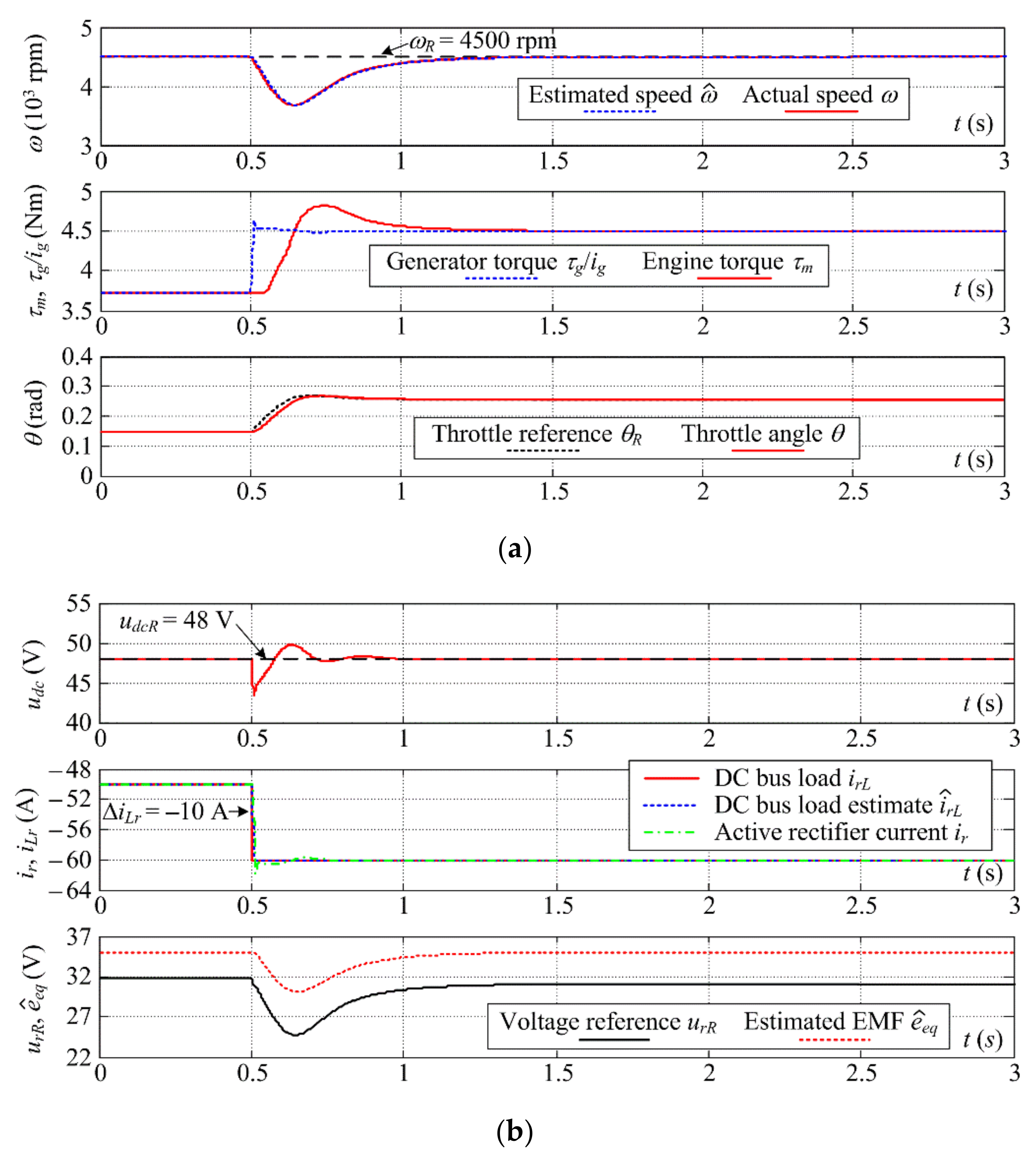
The engine speed control system with PID controller is capable of suppressing the load disturbance within 1 s, with only a moderate engine speed drop of 15.6% from the target value of 4500 rpm;
(ii)
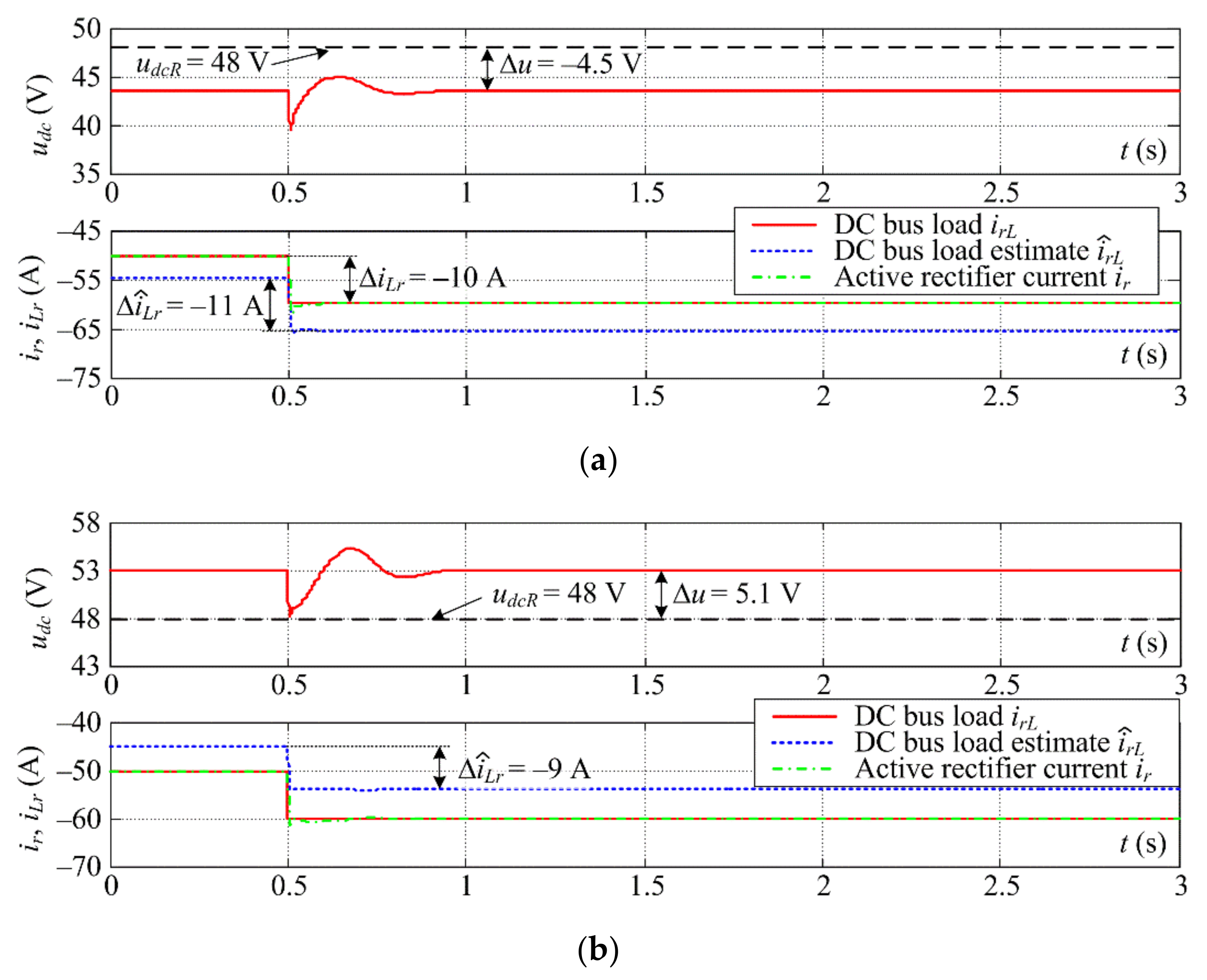
The DC bus voltage/current control system has been characterized by 80 ms recovery time and 200 ms settling time after the sudden DC bus load change, and is also characterized by a non-emphasized drop in the DC bus voltage (10.4% of the target value of 48 V);
(iii)
The engine-generator set speed control system based on Luenberger estimator of brushless DC machine electromotive force estimation may be affected by the armature resistance variations and the brushless DC generator armature current/voltage sensor gain and offset errors, which may result in perceptible closed-loop steady-state speed control error, but the favorable closed-loop damping of the control system is still largely preserved;
(iv)
The anticipated ranges of voltage and current sensor errors also do not significantly affect the DC bus voltage closed-loop system robustness, i.e., favorable closed-loop damping is also preserved. In both cases (i.e., speed control and DC bus voltage control), the control error magnitude is primarily related to magnitudes of the sensor offset errors.
Based on these insights, the overall control system of such hybrid power-plant should be characterized by favorable closed-loop dynamics and acceptable levels of steady-state control errors, whose relative magnitude solely depends on respective sensor characteristics (i.e., gain and offset errors). Moreover, the proposed control systems for the prospective hybrid UAV power-plant should also be characterized by well-damped transient behavior with respect to sudden change in the DC bus load, and rather fast and effective load disturbance recovery.

7. Conclusions

The paper has presented the detailed control system design and robustness analysis for the hybrid propulsion system suitable for unmanned aerial vehicles, which is based on internal combustion engine plus brushless DC generator set power supply of the common DC bus used for power distribution within the aircraft. The overall control system has featured (i) the internal combustion engine speed control system based on a PID feedback controller and (ii) the brushless DC generator active rectifier voltage/current control based on PI feedback controllers, with both feedback loops also featuring load disturbance estimators based on the Luenberger estimator methodology. The design of feedback control systems and estimators has been based on damping optimum criterion which yields straightforward analytical expressions for controller and estimator parameters. The robustness of the proposed control systems to process model parameter variations has been analyzed by closed-loop root locus plots, which have indicated that favorable closed-loop damping obtained through controller/estimator tuning according to damping optimum criterion ought to be preserved for the anticipated range of modeling errors.
The effectiveness of the proposed hybrid propulsion control system suitable for UAV applications has been verified by means of comprehensive simulations. Results have pointed out that the overall control system is characterized by rather fast and effective recovery with respect to load disturbance from the common DC bus, with the “slower” engine speed control system being characterized by approximately 1 s long engine speed recovery transient, whereas the “faster” DC bus voltage control system is capable of recovering the DC bus voltage in approximately 80 ms, with both control loops suffering only moderate excursions from their respective set-point (reference) values. These control system characteristics have been achieved due to accurate and fast estimation of key hybrid propulsion system variables, i.e., engine-generator set speed and electromotive force, and DC bus load, thus enabling effective suppression of control system external disturbances. Moreover, the simulation analysis has also largely confirmed the results of robustness analysis in terms of closed-loop systems maintaining their favorable closed-loop damping properties. Finally, the simulation study has also pointed out to the existence of closed-loop steady-state control errors in both engine speed and DC bus voltage when voltage and current sensor gain and offset errors are present. These errors still have limited magnitudes which are primarily related to magnitudes of sensor offset errors, which directly affect the engine-generator set speed estimation accuracy within the Luenberger estimator and the steady-state accuracy of the DC bus voltage feedback.
Future work may involve designing the upper-level supervisory control strategy aimed at hybrid power-plant energy management and power flow control and building a down-scaled laboratory setup of the hybrid propulsion system for the purpose of experimental verification of individual control system components and overall hybrid power system control strategy.

Author Contributions

Conceptualization, M.K. and D.P.; methodology, D.P., M.K., M.C. and J.B.; software, D.P. and M.C.; validation, D.P. and M.K.; formal analysis, D.P.; investigation, D.P. and M.K.; resources, M.C.; writing—original draft preparation, D.P.; writing—review and editing, M.K., D.P., J.B. and M.C.; visualization, D.P. and M.K.; supervision, M.C.; project administration, D.P.; funding acquisition, D.P. All authors have read and agreed to the published version of the manuscript.

Funding

It is gratefully acknowledged that this research has been supported by the EU European Regional Development Fund under the Grant KK.01.1.1.01.0009 (DATACROSS).

Institutional Review Board Statement

Not applicable.

Informed Consent Statement

Not applicable.

Data Availability Statement

Research data can be made available for non-profit use in research and education upon a formal request made to the corresponding author.

Acknowledgments

We would like to pay our gratitude and our respects to our colleague, Davor Zorc, who has actively supported this research until his untimely passing away in June of 2020. He was a tenured professor at the Department of Robotics and Production System Automation at the Faculty of Mechanical Engineering and Naval Architecture, University of Zagreb, Croatia.

Conflicts of Interest

The authors declare no conflict of interest. The funding body had no role in the design of the study; in the collection, analyses, or interpretation of data; in the writing of the manuscript, or in the decision to publish the results.

Nomenclature

Abbreviations:
ACAlternating current
BLDCBrushless direct current (machine/generator)
BPTTBack propagation through time (gradient optimization)
DC Direct current
DPDynamic programming
ECMSEquivalent consumption minimization strategy
EMFElectromotive force
ICEInternal combustion engine
PIProportional-integral (controller)
PIDProportional-integral-derivative (controller)
PWMPulse-width modulation
rpmRevolutions per minute
UAVUnmanned aerial vehicle
D1 … D6Flywheeling diodes
Q1 … Q6MOSFET switches
Variables:
eeqBLDC machine DC model equivalent electromotive force
elBLDC machine electromotive force per phase
dR, dActive rectifier duty cycle reference and actual duty cycle value
i1, i2, i3Instantaneous values of BLDC machine phase currents
ieq, ieqmBLDC machine DC model equivalent current and its measurement
ir, irLActive rectifier output current and DC bus load current
IphBLDC machine phase current magnitude
pmICE manifold pressure
sLaplace operator
udc, udcmDC bus voltage and its measurement value
urActive rectifier output voltage (line voltage of two BLDC phases)
Wi, WoICE manifold intake and output air mass flow
αgGenerator rotor position
θ, θRThrottle servodrive position and position reference (target)
τm, τL, τgEngine torque, engine load torque and BLDC generator torque
τmaxEngine maximum torque
ω, ωgEngine speed and BLDC generator speed
Parameters:
aω1 … aω5ICE speed closed-loop characteristic polynomial coefficients
CdcDC bus capacitance
D2, …, DnDamping optimum characteristic ratios
D2o, D2LDamping optimum characteristic ratios in estimator design
D2i, D3iDamping optimum characteristic ratios (current PI controller)
D2u, D3uDamping optimum characteristic ratios (voltage PI controller)
D2ω, D3ω, D4ωDamping optimum characteristic ratios (ICE speed PID controller)
igGearbox transmission ratio
JtTotal moment of inertia at engine side
Kci, TciCurrent PI controller proportional gain and integral time constant
Kcu, TcuVoltage PI controller proportional gain and integral time constant
Kdce, KLeCorrection gains of Luenberger estimator (DC bus load estimation)
KeBLDC machine per phase electromotive force constant
Kee, KieCorrection gains of Luenberger estimator (engine speed estimation)
KeqBLDC machine DC model electromotive force and torque constant
Kmt, KpEngine torque equivalent gain and engine “pumping” gain
KR ICE speed PID controller proportional gain
TI, TDICE speed PID controller integral and derivative time constants
lGenerator phase sequence number (1, 2, or 3)
mNumber of generator phases
nClosed-loop system order
pBLDC machine number of pole pairs
RGas constant
Rph, LphBLDC machine phase resistance and inductance
rdSemiconductor “switch” dynamic resistance
Req, LeqEquivalent resistance and inductance of BLDC machine DC model
TSampling time (discrete-time controller)
TmICE manifold time constant
TdICE torque development delay (dead-time)
TeEquivalent closed-loop time constant (damping optimum criterion)
Tei, TeuEquivalent time constants (current and voltage control systems)
TeL, TeoEquivalent time constants in Luenberger estimator designs
TEquivalent time constants (ICE speed control system)
TfCurrent and voltage sensor filtering time constant
TFFeed-forward compensator “lead” time constant
Tpi, TpuParasitic time constants in current and voltage PI controller
Tsw, fswPWM voltage switching delay and switching frequency
Tθ, TΣθThrottle servodrive lag and equivalent lag in PID controller design
TΣiLag of PWM switching and sampling in current PI controller design
TΣuCurrent control loop and sampling lag (voltage PI controller design)
V, ϑICE intake manifold volume and temperature
αFeed-forward compensator filtering pole scaling factor
φmBLDC machine rotor field flux in the gerenal case
φmnConstant value of rectangular field flux spatial distribution
πLudolph’s number (3.1415926)
ζDamping ratio
Symbols:
Estimated variable
_Average value

References

  1. Maza, I.; Caballero, F.; Capitán, J.; Martínez-De-Dios, J.R.; Ollero, A. Experimental results in multi-UAV coordination for disaster management and civil security applications. J. Intell. Robot. Syst. 2011, 61, 563–585. [Google Scholar] [CrossRef]
  2. Kingston, D.; Beard, R.W.; Holt, R.S. Decentralized perimeter surveillance using a team of UAVs. IEEE Trans. Robot. 2008, 24, 1394–1404. [Google Scholar] [CrossRef] [Green Version]
  3. Adams, S.M.; Levitan, M.L.; Friedland, C.J. High resolution imagery collection for post-disaster studies utilizing unmanned aircraft systems (UAS). Photogramm. Eng. Remote Sens. 2014, 80, 1161–1168. [Google Scholar] [CrossRef] [Green Version]
  4. Ayele, Y.Z.; Aliyari, M.; Griths, D.; Droguett, E.L. Automatic crack segmentation for UAV-assisted bridge inspection. Energies 2020, 13, 6250. [Google Scholar] [CrossRef]
  5. Deng, C.; Wang, S.; Huang, Z.; Tan, Z.; Liu, J. Unmanned aerial vehicles for power line inspection: A cooperative way in platforms and communications. J. Commun. 2014, 9, 687–692. [Google Scholar] [CrossRef] [Green Version]
  6. Huang, Y.; Hoffmann, W.C.; Lan, Y.; Wu, W.; Fritz, B.K. Development of a spray system for an unmanned aerial vehicle platform. Appl. Eng. Agric. 2014, 25, 803–809. [Google Scholar] [CrossRef]
  7. Boukoberine, M.N.; Zhou, Z.; Benbouzid, M. A critical review on unmanned aerial vehicles power supply and energy management: Solutions, strategies, and prospects. Appl. Energy 2019, 255, 113823. [Google Scholar] [CrossRef]
  8. Pang, T.; Peng, K.; Lin, F.; Chen, B.M. Towards long-endurance flight: Design and implementation of a variable-pitch gasoline-engine quadrotor. In Proceedings of the IEEE International Conference on Control and Automation (ICCA 2016), Kuching, Malaysia, 23–27 May 2016; pp. 767–772. [Google Scholar]
  9. Sheng, S.; Sun, D. Control and optimization of a variable-pitch quadrotor with minimum power consumption. Energies 2016, 9, 232. [Google Scholar] [CrossRef]
  10. Hung, J.Y.; Gonzalez, L.F. On parallel hybrid-electric propulsion system for unmanned aerial vehicles. Prog. Aerosp. Sci. 2012, 51, 1–17. [Google Scholar] [CrossRef] [Green Version]
  11. Lu, W.; Zhang, D.; Zhang, J.; Li, T.; Hu, T. Design and implementation of a gasoline-electric hybrid propulsion system for a micro triple tilt-rotor VTOL UAV. In Proceedings of the 6th Data Driven Control and Learning Systems Conference, Chongqing, China, 16 October 2017; pp. 433–438. [Google Scholar]
  12. Fredericks, W.J.; Moore, M.D.; Busan, R.C. Benefits of hybrid-electric propulsion to achieve 4x cruise efficiency for a VTOL UAV. In Proceedings of the 2013 International Powered Lift Conference, Los Angeles, CA, USA, 12–14 August 2013; p. 21. [Google Scholar]
  13. Cipek, M.; Pavković, D.; Petrić, J. A control-oriented simulation model of a power-split hybrid electric vehicle. Appl. Energy 2013, 101, 121–133. [Google Scholar]
  14. Abdul Sathar Eqbal, M.; Fernando, N.; Marino, M.; Wild, G. Hybrid propulsion systems for remotely piloted aircraft systems. Aerospace 2018, 5, 34. [Google Scholar] [CrossRef] [Green Version]
  15. Friedrich, C.; Robertson, P.A. Hybrid-electric propulsion for aircraft. J. Aircr. 2015, 52, 176–189. [Google Scholar] [CrossRef]
  16. Finger, D.F.; Braun, C.; Bil, C. A Review of Configuration Design for Distributed Propulsion Transitioning VTOL Aircraft. In Proceedings of the 2017 Asia-Pacific International Symposium on Aerospace Technology (APISAT 2017), Seoul, Korea, 16–18 October 2017; p. 15. [Google Scholar]
  17. Recoskie, S.; Fahim, A.; Gueaieb, W.; Lanteigne, E. Hybrid power plant design for a long-range dirigible UAV. IEEE Trans. Mechatron. 2013, 19, 606–614. [Google Scholar] [CrossRef]
  18. Recoskie, S.; Fahim, A.; Gueaieb, W.; Lanteigne, E. Experimental testing of a hybrid power plant for a dirigible UAV. J. Intell. Robot. Syst. 2013, 69, 69–81. [Google Scholar] [CrossRef]
  19. Depcik, C.; Cassady, T.; Collicott, B.; Burugupally, S.P.; Li, X.; Alam, S.S.; Hobeck, J. Comparison of lithium ion batteries, hydrogen fueled combustion engines, and a hydrogen fuel cell in powering a small Unmanned Aerial Vehicle. Energy Convers. Manag. 2020, 207, 112514. [Google Scholar] [CrossRef]
  20. Benić, Z.; Krznar, M.; Kotarski, D. Mathematical modelling of unmanned aerial vehicles with four rotors. Interdiscip. Descr. Complex Syst. 2016, 14, 88–100. [Google Scholar] [CrossRef]
  21. Wang, X.; Liu, J.; Zhang, Y.; Shi, B.; Jiang, D.; Peng, H. A unified symplectic pseudospectral method for motion planning and tracking control of 3D underactuated overhead cranes. Int. J. Robust Nonlinear Control 2019, 29, 1–18. [Google Scholar] [CrossRef]
  22. Peng, H.; Li, F.; Liu, J.; Ju, Y. A symplectic instantaneous optimal control for robot trajectory tracking with differential-algebraic equation models. IEEE Trans. Ind. Electron. 2020, 67, 3819–3829. [Google Scholar] [CrossRef] [Green Version]
  23. Li, F.; Peng, H.; Song, X.; Liu, J.; Tan, S.; Ju, Z. A physics-guided coordinated distributed MPC method for shape control of an antenna reflector. IEEE Trans. Cybern. 2021, 1–13. [Google Scholar] [CrossRef]
  24. Guemri, M.; Neffati, A.; Caux, S.; Ngueveu, S.U. Management of distributed power in hybrid vehicles based on D.P. or Fuzzy Logic. Optim. Eng. 2014, 15, 993–1012. [Google Scholar] [CrossRef]
  25. Cipek, M.; Kasać, J.; Pavković, D.; Zorc, D. A novel cascade approach to control variables optimisation for advanced series-parallel hybrid electric vehicle power-train. Appl. Energy 2020, 276, 115488. [Google Scholar] [CrossRef]
  26. Esser, A.; Eichenlaub, T.; Schleiffer, J.E.; Jardin, P.; Rinderknecht, S. Comparative evaluation of powertrain concepts through an eco-impact optimization framework with real driving data. Optim. Eng. 2021, 22, 1001–1029. [Google Scholar] [CrossRef]
  27. Sinoquet, D.; Rousseau, G.; Milhau, Y. Design optimization and optimal control for hybrid vehicles. Optim. Eng. 2011, 12, 199–213. [Google Scholar] [CrossRef] [Green Version]
  28. Škugor, B.; Deur, J.; Cipek, M.; Pavković, D. Design of a power-split hybrid electric vehicle control system utilizing a rule-based controller and an equivalent consumption minimization strategy. Proc. Inst. Mech. Eng. Part. D J. Automob. Eng. 2014, 228, 631–648. [Google Scholar] [CrossRef]
  29. Jimenez, P.; Lichota, P.; Agudelo, D.; Rogowski, K. Experimental validation of total energy control system for UAVs. Energies 2020, 13, 14. [Google Scholar] [CrossRef] [Green Version]
  30. Ulsoy, A.G.; Peng, H.; Çakmakci, M. Automotive Control Systems; Cambridge University Press: New York, NY, USA, 2012; pp. 126–130. [Google Scholar]
  31. Deur, J.; Ivanović, V.; Pavković, D.; Jansz, M. Identification and speed control of si engine for idle operating mode. In Proceedings of the SAE 2004 World Congress, Detroit, MI, USA, 8–11 March 2004; SAE Technical Paper No. 2004-01-0898. p. 12. [Google Scholar]
  32. Langouët, H.; Métivier, L.; Sinoquet, D.; Tran, Q.H. Engine calibration: Multi-objective constrained optimization of engine maps. Optim. Eng. 2011, 12, 407–424. [Google Scholar] [CrossRef]
  33. Lin, C.E.; Supsukbaworn, T.; Huang, Y.C.; Jhuang, K.T.; Li, C.H.; Lin, C.Y.; Lo, S.Y. Engine controller for hybrid powered dual quad-rotor system. In Proceedings of the 41st Annual Conference of the IEEE Industrial Electronics Society, Yokohama, Japan, 9–12 November 2015; pp. 1513–1517. [Google Scholar]
  34. Pavković, D.; Deur, J.; Kolmanovsky, I. Adaptive Kalman filter-based load torque compensator for improved SI engine idle speed control. IEEE Trans. Control Syst. Technol. 2009, 17, 98–110. [Google Scholar] [CrossRef]
  35. Schröder, D. Elektrische Antriebe-Regelung von Antriebssystemen; Springer: Berlin/Heidelberg, Germany, 2007; pp. 814–865. [Google Scholar]
  36. Carev, V.; Roháč, J.; Šipoš, M.; Schmirler, M. A multilayer brushless DC motor for heavy lift drones. Energies 2021, 14, 2504. [Google Scholar] [CrossRef]
  37. Pajchrowski, T.; Krystkowiak, M.; Matecki, D. Modulation variants in DC circuits of power rectifier systems with improved quality of energy conversion—Part I. Energies 2021, 14, 1876. [Google Scholar] [CrossRef]
  38. Krznar, M.; Piljek, P.; Kotarski, D.; Pavković, D. Modeling, control system design and preliminary experimental verification of a hybrid power unit suitable for multirotor UAVs. Energies 2021, 14, 2669. [Google Scholar] [CrossRef]
  39. Zhang, X.Z.; Wang, Y.N. A novel position-sensorless control method for brushless DC motors. Energy Convers. Manag. 2011, 52, 1669–1676. [Google Scholar] [CrossRef]
  40. Shao, J.; Nolan, D.; Hopkins, T. A novel direct back EMF detection for sensorless brushless DC (BLDC) motor drives. In Proceedings of the 17th Annual IEEE Applied Power Electronics Conference and Exposition (APEC 2002), Dallas, TX, USA, 10–14 March 2002; pp. 33–37. [Google Scholar]
  41. Krznar, M.; Kotarski, D.; Pavković, D.; Piljek, P. Propeller speed estimation for unmanned aerial vehicles using Kalman filtering. Int. J. Autom. Control. 2020, 14, 284–303. [Google Scholar] [CrossRef]
  42. Pavković, D.; Krznar, M.; Cipek, M.; Zorc, D.; Trstenjak, M. Internal combustion engine control system design suitable for hybrid propulsion applications. In Proceedings of the ICUAS 2020 Conference, Athens, Greece, 1–4 September 2020; pp. 1614–1619. [Google Scholar]
  43. Luenberger, D.G. Observing the state of a linear system. IEEE Trans. Mil. Electron. 1964, 8, 74–80. [Google Scholar] [CrossRef]
  44. Naslin, P. Essentials of Optimal Control; Illife Books: London, UK, 1968; Chapter 2. [Google Scholar]
  45. Mathew, T.; Sam, C.A. Modeling and closed-loop control of BLDC motor using an single current sensor. Int. J. Adv. Res. Electr. Eng. Instrum. Eng. 2013, 2, 2525–2531. [Google Scholar]
  46. Williams, B.W. Power Electronics: Devices, Drivers, Applications and Passive Components; McGraw-Hill: New York, NY, USA, 1992; pp. 772–789. [Google Scholar]
  47. Kong, H.; Liu, J.; Cui, G. Study on Field-Weakening Theory of Brushless DC Motor Based on Phase Advance Method. In Proceedings of the 2010 International Conference on Measuring Technology and Mechatronics Automation, Changsha, China, 3–14 March 2010; pp. 583–586. [Google Scholar]
  48. Pavković, D.; Deur, J. Modeling and Control of Electronic Throttle Drive: A practical Approach-from Experimental Characterization to Adaptive Control and Application; Lambert Academic Publishing: Saarbrücken, Germany, 2011; pp. 123–131. [Google Scholar]
  49. Pavković, D.; Lobrović, M.; Hrgetić, M.; Komljenović, A. A Design of Cascade Control System and Adaptive Load Compensator for Battery/Ultracapacitor Hybrid Energy Storage-based Direct Current Microgrid. Energy Convers. Manag. 2016, 114, 154–167. [Google Scholar] [CrossRef]
  50. Pavković, D.; Cipek, M.; Kljaić, Z.; Mlinarić, T.J.; Hrgetić, M.; Zorc, D. Damping Optimum-Based Design of Control Strategy Suitable for Battery/Ultracapacitor Electric Vehicles. Energies 2018, 11, 2854. [Google Scholar] [CrossRef] [Green Version]
  51. Pavković, D.; Šprljan, P.; Cipek, M.; Krznar, M. Cross-axis control system design for borehole drilling based on damping optimum criterion and utilization of proportional-integral controllers. Optim. Eng. 2021, 22, 51–81. [Google Scholar] [CrossRef]
  52. Gu, J.; Ouyang, M.; Li, J.; Lu, D.; Fang, C.; Ma, Y. Driving and braking control of PM synchronous motor based on low-resolution Hall sensor for battery electric vehicle. Chin. J. Mech. Eng. 2013, 26, 1–10. [Google Scholar] [CrossRef]
  53. Krznar, M. Modelling and Control of Hybrid Propulsion Systems for Multirotor Unmanned Aerial Vehicles. Ph.D. Dissertation, Faculty of Mechanical Engineering and Naval Architecture, University of Zagreb, Zagreb, Croatia, 2020. [Google Scholar]
  54. FoxTech Co. Available online: https://www.foxtechfpv.com/t-motor-u12ii-kv120.html (accessed on 5 July 2021).
  55. DSS2x101-02A High Performance Schottky Diode; Data Sheet No. 20110603A; IXYS Corp.: Leiden, The Netherlands, 2011. [Google Scholar]
  56. Titan ZG 45PCI-HV. Technical Manual; Tony Clark GmbH: Luebbecke, Germany, 2012.
  57. Cipek, M.; Petrić, J.; Pavković, D. A Novel Approach to Hydraulic Drive Sizing Methodology and Efficiency Estimation based on Willans Line. J. Sustain. Dev. Energy Water Environ. Syst. 2019, 7, 155–167. [Google Scholar] [CrossRef]
Figure 1. Schematic layout of the hypothetical hybrid propulsion-based UAV.
Energies 14 07125 g001
Figure 2. Mean value engine model (MVEM) of the internal combustion engine (a), and corresponding linearized model in the vicinity of ICE operating point (b).
Energies 14 07125 g002
Figure 3. Electrical schematic of the BLDC machine with active rectifier at common DC bus (a) and current and voltage waveforms for simultaneous conducting of two BLDC generator phases (b).
Energies 14 07125 g003
Figure 4. The averaged equivalent DC model of the brushless DC machine with simplified model of connection to the DC bus via a PWM-controlled switch-mode power converter (active rectifier).
Energies 14 07125 g004
Figure 5. Block-diagram representation of the Luenberger estimator for rotary speed estimation based on brushless DC armature equivalent DC model.
Energies 14 07125 g005
Figure 6. Block diagram of the linearized engine speed control system with PID feedback controller.
Energies 14 07125 g006
Figure 7. Block diagram representation of the brushless DC machine current control system (a) and DC bus voltage control system (b).
Energies 14 07125 g007aEnergies 14 07125 g007b
Figure 8. Root locus plots of the BLDC generator current control system dominant closed-loop poles subject to armature resistance variations.
Energies 14 07125 g008
Figure 9. Block diagram of the DC bus voltage control system subject to voltage and current sensor errors.
Energies 14 07125 g009
Figure 10. Root locus plots of DC bus voltage control system dominant closed-loop poles subject to voltage/current sensor gain errors.
Energies 14 07125 g010
Figure 11. Locations of dominant closed-loop poles of the linearized ICE speed control loop subject to manifold time constant error (a) and torque gain error (b).
Energies 14 07125 g011
Figure 12. Static maps of the MVEM model used in simulations.
Energies 14 07125 g012
Figure 13. Closed-loop responses of the proposed hybrid propulsion control system for abrupt DC bus load change (nominal case–no modeling and sensor errors): engine quantities (a) and DC bus quantities (b).
Energies 14 07125 g013
Figure 14. Closed-loop responses of engine-generator set speed control system based on EMF estimation subject to armature resistance error ΔReq/Req = −0.25, sensor offset errors Δurm = 0.2 V and Δieqm = 0.2 A, and sensor gain errors: εi = εu = 0.1 (a), and εi = εu = −0.1 (b).
Energies 14 07125 g014
Figure 15. Closed-loop responses of the DC bus voltage control system subject to sensor offset errors Δudcm = 0.2 V and Δirm = 0.2 A and sensor gain errors: εi = εu = 0.1 (a), and εi = εu = −0.1 (b).
Energies 14 07125 g015
Table 1. DC bus connection sequence of phase windings with respect to rotor electrical angle.
Electrical Angle g0–π/3π/3–2π/32π/3–ππ–4π/34π/3–5π/35π/3–2π
Stator phases connected to DC bus1 and 33 and 23 and 22 and 12 and 11 and 3
Table 2. Parameters of linearized process models, estimators and controllers used in simulations.
SymbolDescriptionValue
KeqBLDC machine equivalent EMF/torque gain0.24 Vs/rad
LeqBLDC machine equivalent inductance0.2 mH
ReqBLDC machine equivalent resistance49.4 mΩ
pBLDC machine number of pole pairs4
rdDynamic resistance of semiconductor switch/diode2.7 mΩ
CdcRectifier DC bus capacitance10 mF
TfCurrent/voltage filter time constant1 ms
ϑICE intake air temperature303 K
RUniversal gas constant287 J/(Kg⋅K)
VICE intake manifold volume100 cm3
KmtICE torque development gain10 Nm/rad
TmICE intake manifold time constant10 ms
TdICE combustion delay26.7 ms
TθICE throttle unit delay25 ms
JtOverall inertia at ICE shaft10−3 kgm2
KpICE “pumping” gain10−4 s
igGenerator vs. ICE gearbox ratio3.2
KciBLDC generator current PI controller proportional gain0.055
TciBLDC generator current PI controller integral time constant3.3 ms
KcuDC bus voltage PI controller proportional gain0.611
TcuDC bus voltage PI controller integral time constant40.9 ms
KREngine speed PID controller proportional gain0.00085
TIEngine speed PID controller integral time constant0.217 s
TDEngine speed PID controller derivative time constant0.014 s
KieBLDC generator speed estimator gain (current update)7.53 A/A
KeeBLDC generator speed estimator gain (EMF update)27.44 V/A
KLeDC bus load estimator gain (load current update)800 A/V
KdceDC bus load estimator gain (DC bus voltage update)400 V/V
Publisher’s Note: MDPI stays neutral with regard to jurisdictional claims in published maps and institutional affiliations.

