Abstract
Power system operators are confronted with a multitude of new forecasting tasks to ensure a constant supply security despite the decreasing number of fully controllable energy producers. With this paper, we aim to facilitate the selection of suitable forecasting approaches for the load forecasting problem. First, we provide a classification of load forecasting cases in two dimensions: temporal and hierarchical. Then, we identify typical features and models for forecasting and compare their applicability in a structured manner depending on six previously defined cases. These models are compared against real data in terms of their computational effort and accuracy during development and testing. From this comparative analysis, we derive a generic guide for the selection of the best prediction models and features per case.
1. Introduction
The transition to renewable energy sources for the generation of electricity has strong implications for electricity markets. In contrast to conventional power plants, the output of the majority of renewables is more volatile, as it is strongly dependent on weather conditions. On the one hand, the market value of variable renewable energy source (VRES) is affected by the uncertainty of its output, as forecast errors need to be balanced with short lead times, which imply higher balancing costs [1]. On the other hand, the marginal costs of VRES are often close to zero, and therefore lower the overall electricity market value whenever they are available. The application of more advanced forecasting models poses one possible mitigation strategy to counteract the increased balancing costs of VRES and thereby to increase their market values. By reducing the forecast error, the extent of day-ahead positions that need to be adjusted in the intraday or imbalance market at adverse prices can be reduced [2]. In addition to that, reduced forecast errors for longer lead times increase the number of assets that can ramp their capacities up or down and therefore increase the number of available flexibility options, leading to lower balancing costs. This can be explained by the better observability of limitations stemming from ramp-up and ramp-down times of conventional power plants [3].
Several socio-economic trends further emphasize the increasing need for more advanced forecasting techniques in addition to the expansion of VRES. The increasing grid loads that result from electric mobility and electric heating need to be closely monitored to take countermeasures such as demand-side management on potential grid congestion. The deregulation of the electric supply industry has led to more conservative infrastructure upgrades, causing a more stressed operation of electrical grids [4].
While first research on load forecasting dates back to the 1960s, selecting the most appropriate model for a specific forecasting scenario has since become a much more difficult task [5]. The majority of research in the subject area is conducted on increasing the accuracy of load forecasts, while the resulting (economic) value of forecasts is rarely addressed [6,7]. A recent review on energy forecasting [8] reveals that few research contributions deal with residual load forecasting. For load forecasting in operational grid planning though, on-site energy generation is of utmost importance. To incorporate the intermittent energy generation, the grid operators can either aggregate separate models dedicated for each domain, generation and load, or make use of integrated forecasting methods that deliver directly a residual load forecast. In some cases, it is not possible to separate generation forecasting and load forecasting, for instance, when the metering data only provide net metering information. This is mostly the case when dealing with smaller microgrid type of grid structures with few monitoring devices; the work in [9] considers a set of forecasting models (a naïve persistence model, an autoregressive model and an Artificial Neural Network (ANN) model) and shows that the integrated approach outperforms the additive one. Due to missing separation of generation and load metering data researches, the authors of [10,11] have explored further integrated models by applying machine learning models (ANNs and Recurrent Neural Networks (RNNs), in particular) for residual load forecasting. Thus, the present study focuses on the evaluation of integrated residual load forecasting models to predict the energy consumption in a section of the electrical grid that is not covered by controllable and intermittent local energy supply. Note that this largely influences the predictive performance of the forecasting models under study due to the larger uncertainty of the prediction variable. In order to conduct a systematic and comprehensive comparative analysis of forecasting method accuracies and their economic value, first a generic methodology must be available upon which different forecasting methods can be evaluated. One missing element in such an holistic economic study (e.g., as undertaken in [12]) is a fundamental preparation of potential forecasting method candidates. Thus, the present work contributes a generic guide for the feature and model selection to facilitate the parametrization needs in the development of forecast models for day-ahead (DA), intraday (ID) and imbalance (IB) markets over two use case dimensions—the forecast horizon and the load aggregation level—to facilitate targeted power operation and planning, from a broader scope.
The forecasting horizon is analyzed in the categories of (i) very short-term load forecasting (VSTLF) with predictions up to one hour ahead, (ii) short-term load forecasting (STLF) for day-ahead predictions and (iii) medium-term load forecasting (MTLF) for forecasts up to one month ahead. We study this dimension, as varying input variables affect the load forecasts for different lead times. Forecasts with very short horizons usually consider historical load values as their only input factor. In contrast, short-term and medium-term forecasts typically also take exogenous variables such as time factors or meteorological data into account. Therefore, the selection of an appropriate prediction approach is highly dependent on the respective forecast horizon [13].
The second dimension, the aggregation level (also known as the hierarchical dimension [14]), has an important impact on the forecast quality, as aggregated loads tend to be more predictable. Therefore, typically, the individual consumption patterns of customers are increasingly smoothed out, the more consumers are combined into one load [15]. As part of this work, we evaluate a total of three Swedish distribution system datasets on three aggregation levels within the same region:
- High: exemplified by net load forecasts for a high voltage (EHV/HV) distribution node.
- Medium: exemplified by net load forecasts for a (HV/MV) node to a local geographical island.
- Low: exemplified by net load forecasts for a large residential customer.
The literature is manifold on up-to-date surveys [16] and performance studies [14,17,18] of advances in the application of forecasting for specific use cases. Further, several studies exist that compare forecasting techniques across one of the above-mentioned dimensions [14,15]. To the best of our knowledge, though, there is no publication that evaluates a variety of the most common forecast models across both the temporal and the aggregation dimension, in order to derive recommendations for the appropriate selection for a given load forecasting problem. The expected learning outcome is that potentially already existing forecasting methods in the system operators’ control room are very well suited for use with related forecasting problems. Thus, the motivation for this study is to elaborate on the research gap concerning the transferability of well-performing forecasting methods across different aggregation levels and different time horizons.
2. Materials and Methodology
In this study, we focus on forecasts that are used by power system operators for operational tasks covering up to one year, i.e., categorized as VSTLF, STLF and MTLF [14]. As the influence of external economic and demographic effects increases for longer forecasting horizons, we limit the horizon of forecasts in the group of MTLF to one month ahead. Table 1 summarizes the forecasting horizons investigated in this paper.

Table 1.
Examined forecasting horizons with corresponding cut-off times and data resolutions.
2.1. Datasets and Data Processing
As the goal of this work is a performance comparison of different forecasting models for several load-forecasting horizons and aggregation levels, a total of three different time series datasets that strongly differ in their load pattern characteristics and origins are used. The datasets all originate from the SE4 bidding area in Southern Sweden and contain the residual load data points at an hourly resolution. Here, the residual load (also known as net load) denotes the difference between the system load profile and the feed-in from renewable energy sources, i.e., the load which still has to be covered by conventional power plants [19]. In order to enable forecasts with forecasting horizons of less than one hour ahead, load values and corresponding weather data are interpolated to quarter-hourly resolution for the respective forecasts. Similarly, for MTLF the data are resampled to daily resolution through an aggregation by the average hourly load value of each respective calendar day. While predictions in the categories of VSTLF and STLF are applied for operational purposes, the longer prediction period of MTLF at daily resolution is helpful, e.g., for early mitigation of potential congestion situations via bipartite contracts. To comply with data protection regulation policies, the load levels were normalized in advance using a Min-Max scaler, according to Equation (1):
and are the minimum and maximum load levels measured in the training set of each dataset. As the datasets were all measured for different time periods, the overlapping time frame for which all datasets are available, i.e., 24 January 2017 to 7 March 2019, is reviewed as part of this work. This period comprises a total of 18,552 data points at an hourly resolution. The datasets are labeled according to their aggregation level in the following manner:
- H—High Aggregation Level
- M—Medium Aggregation Level
- L—Low Aggregation Level
Dataset H features residual load levels on the highest aggregation level considered in this work, as they were measured for an extra-high-voltage (EHV) transmission line in Southern Sweden that acts as the link between a larger metropolitan area and the overarching transmission grid. While several power plants and an offshore wind park are part of the regional DSO’s grid, approximately 80% of the total energy demand of the region is supplied through the overlying grid.
Figure 1 shows a recurring pattern of significantly higher energy demand for the winter months and lower consumption levels for the summer months. The daily peak load is measured in the morning hours on weekdays and in the evening hours on weekends, while the weekends show a lower load than the weekdays. The augmented Dickey–Fuller (ADF) test, conducted using Python 3.9 with the statsmodels package and the corresponding tsa.stattools.adfuller function, indicates stationarity for the dataset. Thus, the ARIMA and Exponential-Smoothing (ES) model should be able to predict accurate values without the need for prior differentiation. However, the wide band around the load curve, depicted on the right, shows the high variation in the data over the studied weeks.
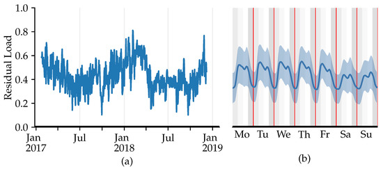
Figure 1.
Residual load curve (a) and average weekly load curve (b) for the high aggregation level (Case H). The area around the load curve (b) represents ±1 standard deviation.
Dataset M originates from an island off the coast of Sweden. The dataset is of particular interest, as the island has a high share of renewable energy sources on the island itself and was able to operate independently from the overlaying grid about 25% of the time in the period under study. The residual load was measured at the sea cable connection between mainland Sweden and the geographical island. The load curve exhibits a constant mean and no salient seasonality. The ADF-test results in a stationary statement. Due to an original lack of weather information, the meteorological information was gathered from the SMHI Open Data API for the station closest to the island.
With reference to the Swedish standard industrial categorization [20], dataset L comprises the load data collected for an apartment building. For this time series dataset, the ADF-test indicates non-stationarity. As the exact location of the customer site is handled confidentially, obtaining data from the closest weather station is not possible. However, it is known that the customer is also connected to the SE4 bidding area in Sweden. Thus, the weather information is taken for the Hästveda station that is closest to the geographical center of the SE4 area, provided by the SMHI platform.
2.2. Implementation
We implemented the different forecasting approaches in Python 3.9, utilizing mainly the statsmodels [21], sklearn [22], and keras modules and frameworks as listed in Table 2.
Table 2.
Utilized Python packages for the implementation of common forecast models.
For our analysis we generated a total of eleven features. While we created these features for each forecast horizon and dataset, not all of the variables are selected as input factors for all models. That is, for each model and forecast horizon, a separate selection from the pool of available features is performed later on. The features most commonly used in the area of load forecasting can be grouped into three distinct categories: (i) past load data, (ii) calendric data and (iii) meteorological data [23]. For the univariate models, we use all past observations as endogenous features. For the other models, we generate a feature that holds the load value lagged by the number of time steps in the forecast horizon. For example, the feature for the 30-day-ahead forecast comprises the load value lagged by 30 days.
For the temporal and calendric feature categories, we use two different approaches. In the first one, we generate one-hot encoded values [24] of the current hour (, weekday () and month (). In addition to that, we generate two cyclic features by applying the trigonometric functions to the hour of the day and the month of the year. This is done in order to bypass potential problems for the one-hot encoded features that numerically suggest a large difference between the beginning and end of each daily, weekly and monthly cycle. Another important factor for the load values on a given day are working days, as the activity of industrial and business customers causes higher energy consumption during the week in comparison to the weekends. In addition to the day-of–the-week feature that we introduced above, we generate a single dummy variable that is equal to one if a day is a working day and zero if it is on a weekend. The feature also considers public holidays in Sweden.
As meteorological information, we include features for the temperature and wind speed as exogenous variables. The corresponding data sources for these features differ for each dataset and have been pointed out as part of the detailed description of the time series in the last section. Similar to the residual load values, both the temperature and windspeed values are normalized using the Min-Max scaler from Equation (1). A summary of all generated features, their corresponding abbreviations and value ranges is given in Table 3.
Table 3.
Overview of all exogenous features.
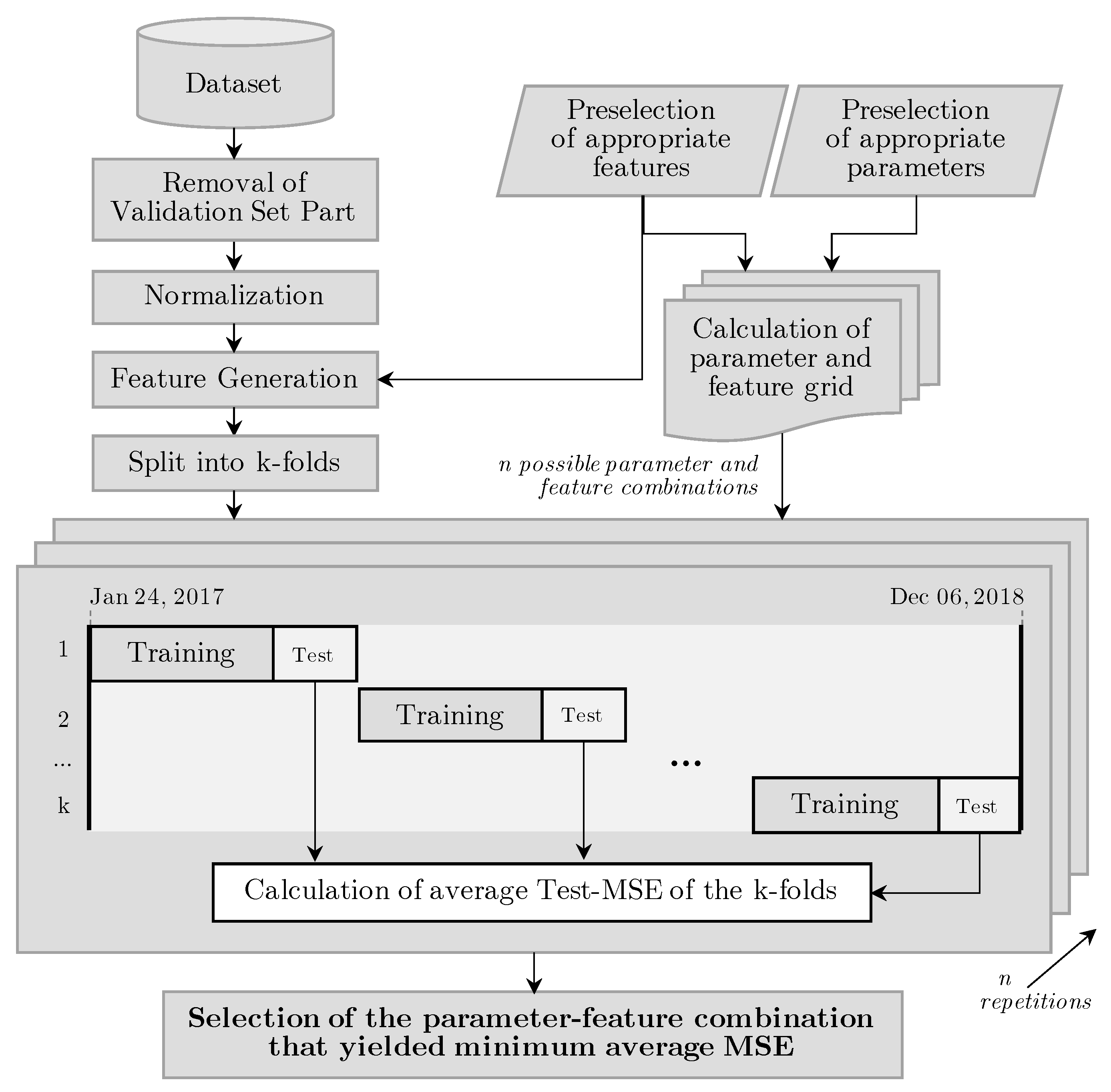
The options for the parameter tuning orange from applying the default values of the software package used, the use of recommendations from the literature regarding tuning strategies that try to minimize an error metric on the test set by analyzing numerous configurations in a defined parameter search space [25]. As part of this work, we derive a set of several possible parameter values for each model from literature recommendations and then measure the resulting accuracy for all possible parameter combinations. The evaluated parameters and the selected values for each model can be found in the Appendix A as part of Table A2, Table A3, Table A4, Table A5, Table A6, Table A7 and Table A8. The entire process of selecting the model parameters and features is shown as a flow chart in Figure 2. We distinguish the so-called first-level model parameters and hyper-parameters which both have to be carefully optimized to achieve an optimal prediction output. First-level model parameters are for instance the order of auto-regression and moving averages in the ARIMA models, while hyperparameters refer to the calibration of the training process in machine learning based methods, such as the RNN.

Figure 2.
Parameter and feature selection process, conducted for each of the models and datasets.
2.3. Validation Approach
The validation parts of the datasets that range from 7 December 2018 to 7 March 2019 (and were not considered during the model selection stage) are therefore utilized to simulate the model predictions on newly added data. For this, an expanding window approach as shown in Figure 3 is applied to each parametrized model. In the first step, all observations including the full training and validation parts of the datasets are loaded into the system. The observations are then normalized using the Min-Max-Scaler (see: Section 2.1). In order to avoid any bias from knowing future load values, the Min-Max-Scaler is applied using the parameter values (i.e., the minimum and maximum loads) from the training part of the dataset instead of those of the validation set. In addition to the meteorological features of temperature and wind speed that are already included in the datasets, the temporal features are generated, provided they have been selected for a specific model. The models are then initialized using the parameter configurations that showed the best performance on the training set.
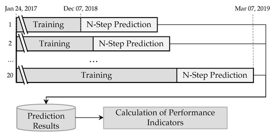
Figure 3.
Validation approach for each of the selected models.
Twenty expanding windows are then used to evaluate the model performances: While in the first window, only the observations of the training dataset are used for the model fitting, the second expanding window also uses the observations from the validation set-up to the beginning of the expanding window for the model training. This approach is used because the autoregressive models that are part of this work produce accurate predictions for a short period of time but tend to become inaccurate when the time period between the last observation used for the model fitting and the prediction target grows. By adding newer observations in every new window, the accuracy of the models can be evaluated for a relevant forecasting horizon for multiple times. In each window, the fitted model is performing a prediction for a predefined number of future time steps, e.g., 30 days for the MTLF case. The number of windows was selected arbitrarily as a trade-off between calculation time and biases due to a small sample size. By evenly distributing the 20 windows across different hours of day and days of the week, potential statistical biases are further minimized.
The model predictions are saved separately for each window. This then allows the evaluation of error metrics such as the mean squared error (MSE) and mean absolute error (MAE) as an average of the prediction of the 20 windows. As residual loads that can show values close or equal to zero are forecasted in this work, relative metrics show unstable values for our analysis and will therefore not be considered any further. In addition to the predicted load time series, the fitting and prediction times are also captured to allow conclusions about the computational effort during the model development phase.
3. Results and Discussion
The validation set ranges from 7 December 2018 to 7 March 2019 and was not used as part of the model selection. It is therefore utilized to simulate the model predictions on unknown data in order to measure the models’ ability to generalize on the so-called out-of-sample data. We evaluate the prediction accuracy of each model in each case, based on MAE and MSE metrics. Further, we measure the training and prediction times to allow conclusions on the required computational effort during the forecast deployment stage. At this point, due to the fact that our numerical results for the large set of discussed cases are far too many to be reported here in a comprehensive manner, we refer our readers to the result tables in this paper’s appendix (Table A1) and open-source code mentioned in the last paragraph.
To allow a meaningful comparison of the forecasting models selected in the previous section, we now define two naïve forecasting approaches that act as baseline models for a benchmarking of the performance of the more complex forecasting methods. The first naïve model, which we refer to as Naive1, assumes all future values to be equal to the last observed value [26], as given in Equation (2):
The second baseline model (Naive2) assumes the load value to recur periodically based on a defined seasonal period k. The mathematical representation of this model is given in Equation (3):
where m is the number of time steps in one period.
3.1. Very Short-Term Load Forecasting
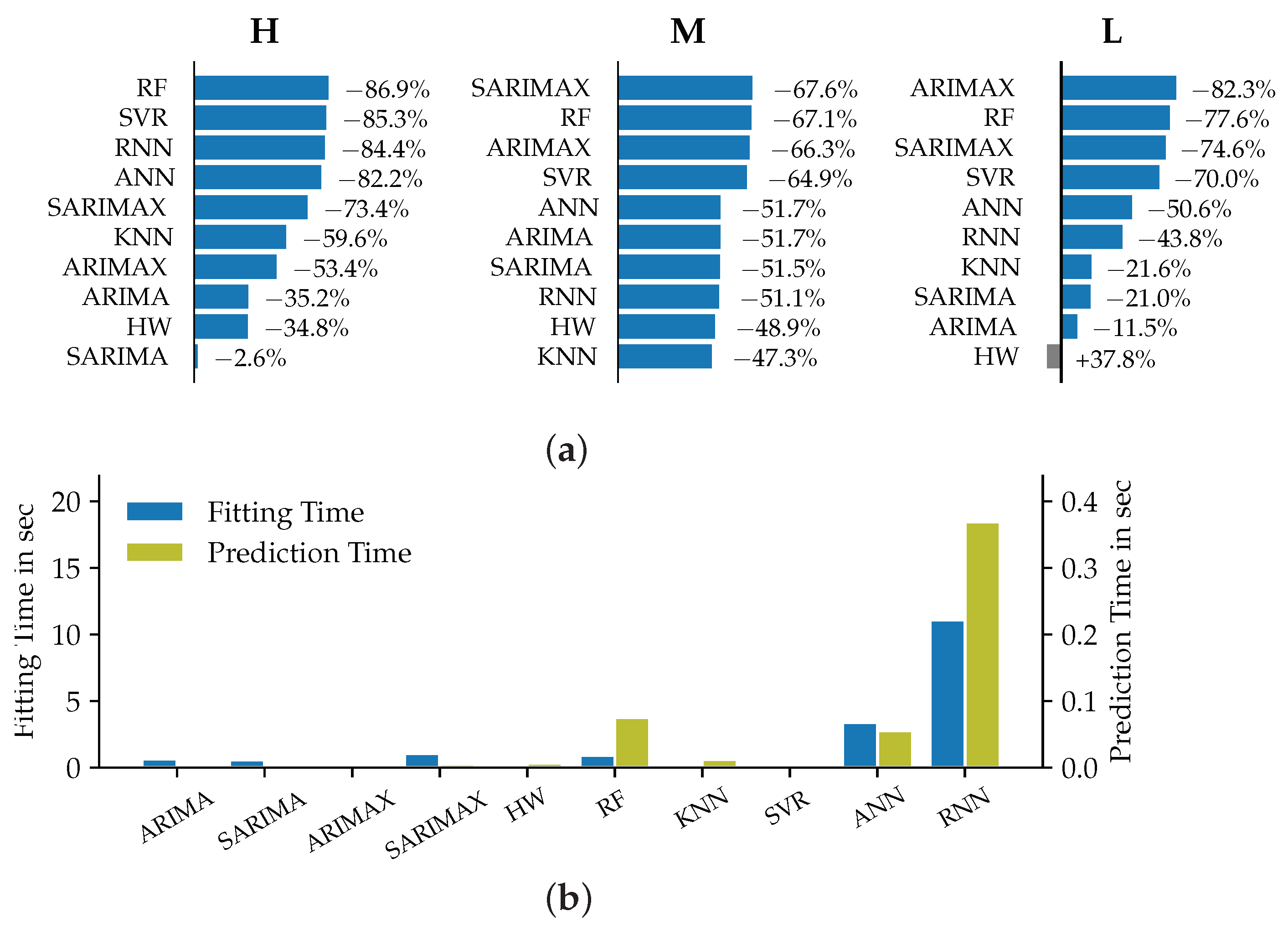
The parametrized VSTLF models predict load values for a lead time of one hour at a quarter-hourly resolution, i.e., a prediction of four discrete time steps ahead is conducted. The accuracy benchmark on the expanding window validation for each model dataset, compared on the basis of MSE, are shown together with the required fitting (FT) and prediction times (PT) per sliding window in Figure 4. The relative improvement compared to the benchmark models is calculated as given in Equation (4):
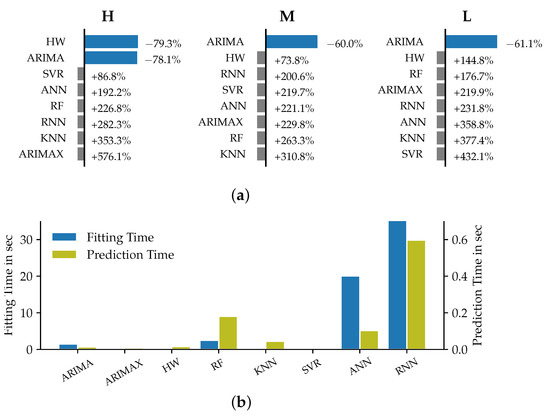
Figure 4.
Relative improvement of the models’ MSE metrics compared to Naive1 (a) and corresponding prediction and fitting times (b) for datasets H, M and L in the VSTLF case.
It can be seen that the ARIMA models were the best-performing ones across the datasets in terms of minimizing the error functions. Aside from the Holt–Winters model for dataset H that scored a slightly lower MSE than the respective ARIMA models, ARIMA always represented the best forecasting approach. As can be seen in the upper part of Figure 4, ARIMA was the only method that outperformed the naïve prediction for all datasets. The average improvement for all datasets in terms of the MSE for ARIMA amounted to 64.1%.
What the ARIMA and HW models have in common is that they do not consider any exogenous predictor variables, i.e., pose univariate methods [27]. We derive from these observations that for the VSTLF case no exogenous variables should be included as part of the forecast. Regarding the model selection, we recommend the consideration of ARIMA and Holt–Winters models for the time horizon of up to one hour. These observations can confirm previous findings, e.g., the results of empirical studies conducted by [28,29]; both found univariate models to outperform more sophisticated approaches for very short time horizons. Our observations also coincide with the variable selection recommendations given by [4] that classify exogenous variables as not required for the VSTLF case.
The seasonal period of 24 × 4 time steps for the VSTLF case is quite long in comparison to the forecast horizon of only four predictions. This entails the effect of a considerably more relevant and accurate Naive1 forecast performance in comparison to the seasonal Naive2 approach. This can be explained by the closer temporal proximity of the last observed load value to the forecast horizon. Consequently, the model performance of the selected models almost entirely outperformed the Naive2 forecast. As this, however, does not come with any practical value for the VSTLF forecast horizon, the in-depth analysis of the comparison with the second naïve model is omitted at this point. The longest fitting and prediction times were observed for the deep neural network approaches of ANN and RNN. The lowest computation times were measured for the univariate time series models (ARIMA and HW) as well as for ARIMAX and Support Vector Regression (SVR). Unexpectedly, we observed ARIMAX models to require shorter times than the corresponding ARIMA models with the same model order but without exogenous variables. We assume the effect to be caused by the use of different regression parameter estimation approaches in the statsmodels implementation when including exogenous variables.
Interestingly, the prediction accuracy did not appear to be overly affected by the load aggregation levels of the respective datasets. Some of the evaluated models, such as HW and KNN, showed increased MSE and MAE values for datasets originating from lower aggregation levels. Other models, including the ARIMA models, scored slightly better in terms of accuracies for the customer load dataset than for the datasets using a medium aggregation level. This finding further emphasizes our recommendation for the use of ARIMA models across all aggregation levels, while we narrow down our recommendation for the use of HW models to the application on highly aggregated loads only.
3.2. Short-Term Load Forecasting
Analyzing the results for the short-term time horizon of one day ahead that are reported in Figure 5, it can be seen that the accuracies of the models showed much more variation across the different datasets. Random Forests showed the best accuracy for the customer dataset L and for the medium aggregation level dataset M. For the high level of aggregation (dataset H), the RF model was outperformed by the SVR model.
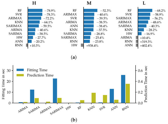
Figure 5.
Relative improvement of the models’ MSE metrics compared to Naive1 (a) and corresponding prediction and fitting times (b) for datasets H, M and L in the STLF case.
The univariate models that performed best in the VSTLF case scored significantly lower in terms of accuracy for the day-ahead forecasting case. This corresponds to the findings in [4], the authors of which state that exogenous predictors, and especially meteorological variables, are required in addition to endogenous load data for accurate STLF forecasts.
Further, Figure 5 shows that the MSE improved for almost all of the evaluated models. This, however, did not apply to the RNN models, which performed worse than the naïve approach in all but one case. The ANN model in comparison showed good performance for the datasets on the high and medium aggregation levels but a poorer performance for the customer datasets. We assume overfitting related to not interrupting the training process early enough to be the cause for the overall fair to medium performances of the deep learning approaches of ANN and RNN. One accuracy outlier can be seen in the performance of the HW model on dataset M. The model was parametrized with a smoothing parameter of . This value was already noticed as possibly being unsuitable during the parameter selection, yet still yielded the smallest MSE on the training part of the dataset. The insufficient performance of the model on the validation dataset is therefore not surprising. Due to the clear seasonality in the load pattern over the course of one day, the SARIMA and SARIMAX models were able to outperform the corresponding non-seasonal ARIMA models. Interestingly, the missing seasonality factor appeared to be substituted by the inclusion of exogenous variables into the regression for dataset H and M, as the ARIMAX models showed considerably higher accuracies. As expected, the MSE appears to increase, the longer the forecast lead time is. This trend is weaker for the neural network models, which might be explained by an overall weak performance of these models in our study. The Holt–Winters model for dataset M that was identified as unsuitable before shows an almost linear increase of the MSE over the lead time.
As the MSE error curves are all relatively close to each other, we cannot observe a specific pattern in the predictability of the different aggregation levels across all models. SARIMA and SARIMAX also showed the lowest accuracies on the medium level for dataset M. The deep learning approaches performed worst for the low aggregation level of dataset L. The findings regarding average required fitting and prediction times match the observations from the VSTLF case. The computational effort for ANN and RNN was among the highest. The SARIMA and SARIMAX models that were not part of the VSTLF also showed relatively long fitting times. This can be explained by the greater number of first-level model parameters that require fitting and stem from the seasonal part in the regression, as compared to the ARIMA models. Random forest regression models show consistently low error metrics across the datasets and also exhibit comparably low computational effort. This combination makes them a highly effective forecasting approach for the STLF time horizon which coincides with the findings in [30].
3.3. Medium-Term Load Forecasting
In contrast to the previously analyzed time horizons, Figure 6 reveals a clear connection between the model accuracies and the load aggregation level of the corresponding datasets. The ARIMAX models performed the best in terms of both MAE and MSE for the low aggregation level of dataset L. SARIMAX models in comparison showed the lowest accuracy in terms of MSE for the medium aggregation level. The best accuracies for the high aggregation level (dataset H) were reached by the machine learning algorithms RF and SVR.

Figure 6.
Relative improvement of the models’ MSE metrics compared to Naive1 (a) and corresponding prediction and fitting times (b) for datasets H, M and L in the MTLF case.
All of the analyzed models for the medium to high aggregation level datasets show a relative reduction of MSE in comparison against Naive1. For the dataset L, merely the models HW, SARIMAX and ANN show decreased accuracy values. Across the datasets, it can be observed that the univariate models of the ARIMA, SARIMA and HW type performed noticeably inferiorly than for the two shorter time horizons. This can be explained by the fact that the only input for these models are historic load values. The further away the predicted time point is from the last observed load value, the higher the forecast error becomes. This also explains the superior performance of the autoregressive models with exogenous predictors as described in the last paragraph. These models receive the value of the predictor variables in each time step and are therefore able to better predict loads for longer lead times. Across all datasets the RF models showed the highest accuracy improvement compared to the naïve models. This underlines our observation from the STLF case of RF models not being overly affected by the aggregation level. As the comparison with the Naive2 forecast leads to the same conclusions, the corresponding graphic is not discussed at this point.
The required fitting and prediction times are considerably lower than for the previously discussed forecast horizons. This can be explained by the overall lower number of samples in the training set, as the datasets were evaluated at a daily resolution for the MTLF case. Despite this observation, the results can be compared to the previous time horizons. The deep neural network models showed the longest fitting times. In terms of prediction times, the RNNs are followed by the RF and ANN models. The seasonal autoregressive models showed shorter fitting times than for the STLF case, which on the one hand may be explained by the data resolution. On the other hand, the length of one seasonal period of seven samples is lower than the 24 samples used in the STLF case. This implies a smaller number of regression parameters to be estimated during the fitting process, leading to lower computational effort. The KNN and SVR models also showed both very low fitting and prediction times. The fitting and prediction time differences might not be significant in absolute terms for our particular datasets. However, the relative differences between them indicate that for larger datasets the choice of model can have a significant impact on the required computational effort and therefore on the necessary hardware.
4. Conclusions and Outlook
Examining the validation results for the developed models, we find univariate models to perform best for the VSTLF of up to one hour ahead. This includes their forecast accuracy as well as the low computational effort needed to fit the models and to perform predictions. While HW showed varying results for the different aggregation levels, ARIMA was able to accurately forecast across all evaluated datasets. Such a clear conclusion could not be drawn for the STLF time horizon of one day ahead. As for this time horizon, a clear seasonal pattern is visible in the load curve, and the autoregressive models SARIMA and SARIMAX showed high accuracies, but required longer model fitting times. Random Forest models also showed consistently low errors, while requiring lower computational effort. All other models exhibited strongly varying accuracies across the evaluated models, which implies the requirement of an in-depth evaluation prior to the application of these approaches on new use cases.
For the MTLF case that predicts load values of up to 30 days ahead, we saw the accuracy of Random Forests to again be consistently high across all aggregation levels. Compared to other approaches however, they showed longer prediction times. ARIMAX models exhibited high accuracies at the low aggregation level, while SARIMAX resulted in lower error metrics for medium aggregation datasets. For the high aggregation level, all machine learning based approaches created forecasts with high accuracies. Especially the SVR model showed extremely low computational effort for this dataset. Therefore, we draw the conclusion that if the computational effort is not of highest priority, RF models should be used for medium-term forecasts. If the prediction times are of high concern, the model should be selected according to the aggregation level of the evaluated dataset.
Interestingly, we observed ANN and RNN models to score relatively low in terms of accuracies across the different time horizons. As we expected them to rank among the best approaches, we assume the reason for this to be overfitting to the training data points. Therefore, our performance results for these specific model types cannot be generalized for the case where data analytics experts are developing the models. Thus, this aspect counts in general against the ease of the application of such advanced forecasting methods in the traditional power system operation business, as they do not serve a highly-accurate model that is usable straight out-of-the-box. All in all, it can be concluded that while we were able to draw some recommendations on the model selection for pre-defined load forecasting tasks, the proposed selection guideline does not boil down to a single solution that would perform well enough for all use cases.
For future studies, we see the need to quantify the economic value of higher performance accuracies and how this may further affect the selection of the optimal forecasting technique for the cases discussed in this work. Materials, Methods and detailed Result Tables available under: https://github.com/leonardbu/energies (accessed on 23 October 2021), doi:10.5281/zenodo.5345621.
Author Contributions
Conceptualization, methodology, software, validation, formal analysis, investigation, resources, data curation, writing—original draft preparation, visualization, editing, project administration L.B., G.G.-T. and R.M.; writing—review and supervision, G.G.-T., R.M. and A.M.; funding acquisition A.M. All authors have read and agreed to the published version of the manuscript.
Funding
This research was funded by European Union’s Horizon 2020 research and innovation programme under grant agreement no. 824414 https://coordinet-project.eu/ (accessed on 23 October 2021).
Institutional Review Board Statement
Not applicable.
Informed Consent Statement
Not applicable.
Data Availability Statement
Not applicable.
Acknowledgments
The authors gratefully acknowledge E.ON Energidistribution for providing data for the realization of the southern Sweden regional forecast in the CoordiNet project.
Conflicts of Interest
The authors declare no conflict of interest.
Abbreviations
The following abbreviations are used in this manuscript:
| ADF | Augmented Dickey-Fuller |
| ANN | Artificial Neural Network |
| API | Low Aggregated Load Case |
| ARIMA | Auto-Regressive Integrated Moving Average |
| ARIMAX | Auto-Regressive Integrated Moving Average Exogenous Variable |
| DA | Day-Ahead |
| DSO | Distribution System Operator |
| EHV | Extra-High Voltage |
| ES | Exponential Smoothing Model |
| FT | Fitting Time |
| H | Highly Aggregated Load Case |
| HV | High Voltage |
| HW | Holt-Winters Model |
| IB | Imbalance Market |
| ID | Intraday Market |
| KNN | K-Nearest Neighbors |
| L | Low Aggregated Load Case |
| M | Medium Aggregated Load Case |
| MAE | Mean Absolute Error |
| MSE | Mean Squared Error |
| MTLF | Medium Term Load Forecasting |
| MV | Medium Voltage |
| PT | Prediction Time |
| RF | Random Forest Model |
| RNN | Recurrent Neural Network |
| SARIMAX | Seasonal Auto-Regressive Integrated Moving Average Exogenous Variable |
| SMHI | Swedish Meteorological and Hydrological Institute |
| STLF | Short-Term Load Forecasting |
| SVR | Support Vector Regression |
| VRES | Variable Renewable Energy Sources |
| VSTLF | Very Short Term Load Forecasting |
Appendix A
Table A1.
Performance indicators for the three forecast horizons (VSTLF, STLF and MTLF) and data sets used (H, M and L).
Table A1.
Performance indicators for the three forecast horizons (VSTLF, STLF and MTLF) and data sets used (H, M and L).
| H | M | L | ||||||||
|---|---|---|---|---|---|---|---|---|---|---|
| VSTLF | STLF | MTLF | VSTLF | STLF | MTLF | VSTLF | STLF | MTLF | ||
| Naive1 | MAE | 0.02191 | 0.10745 | 0.15186 | 0.03191 | 0.10457 | 0.22742 | 0.03200 | 0.10029 | 0.09697 |
| MSE | 0.00081 | 0.01791 | 0.03659 | 0.00178 | 0.01773 | 0.07869 | 0.00170 | 0.01645 | 0.01445 | |
| Naive2 | MAE | 0.07386 | 0.11174 | 0.15885 | 0.08059 | 0.11517 | 0.23853 | 0.17380 | 0.08169 | 0.09489 |
| MSE | 0.00733 | 0.01834 | 0.03768 | 0.01082 | 0.01949 | 0.08585 | 0.03397 | 0.01003 | 0.01352 | |
| ARIMA | MAE | 0.00792 | 0.08354 | 0.12494 | 0.01774 | 0.08490 | 0.15747 | 0.01651 | 0.10471 | 0.09167 |
| MSE | 0.00018 | 0.01065 | 0.02371 | 0.00071 | 0.01091 | 0.03803 | 0.00066 | 0.01816 | 0.01278 | |
| FT | 2.27597 | 1.59910 | 0.37247 | 1.45997 | 2.00909 | 0.43342 | 1.61464 | 0.11611 | 1.23961 | |
| PT | 0.00863 | 0.02415 | 0.00317 | 0.00881 | 0.02438 | 0.00328 | 0.00916 | 0.02209 | 0.00468 | |
| ARIMAX | MAE | 0.06007 | 0.05853 | 0.11117 | 0.06927 | 0.08148 | 0.13169 | 0.05573 | 0.07609 | 0.03925 |
| MSE | 0.00548 | 0.00497 | 0.01704 | 0.00589 | 0.01053 | 0.02652 | 0.00543 | 0.00846 | 0.00256 | |
| FT | 0.29530 | 0.30320 | 0.09219 | 0.32113 | 0.25716 | 0.13118 | 0.29770 | 0.15288 | 0.15240 | |
| PT | 0.00825 | 0.03767 | 0.00436 | 0.00756 | 0.02275 | 0.00506 | 0.00740 | 0.02164 | 0.00468 | |
| HW | MAE | 0.00760 | 0.09248 | 0.12668 | 0.04052 | 0.28814 | 0.15869 | 0.04389 | 0.09525 | 0.11010 |
| MSE | 0.00017 | 0.01294 | 0.02384 | 0.00310 | 0.18413 | 0.04025 | 0.00415 | 0.01368 | 0.01990 | |
| FT | 0.18801 | 0.01566 | 0.00862 | 0.15953 | 0.02042 | 0.01006 | 0.06343 | 0.00547 | 0.00926 | |
| PT | 0.01918 | 0.01100 | 0.00699 | 0.01319 | 0.00841 | 0.00652 | 0.01332 | 0.00404 | 0.00716 | |
| RF | MAE | 0.04211 | 0.05049 | 0.05909 | 0.07296 | 0.07114 | 0.12674 | 0.05678 | 0.05979 | 0.04817 |
| MSE | 0.00265 | 0.00377 | 0.00481 | 0.00648 | 0.00846 | 0.02589 | 0.00469 | 0.00523 | 0.00324 | |
| FT | 3.39467 | 1.26984 | 1.15574 | 2.47612 | 0.30422 | 1.12497 | 4.37455 | 0.65880 | 1.05151 | |
| PT | 0.26120 | 0.09841 | 0.10195 | 0.19809 | 0.02821 | 0.08571 | 0.27926 | 0.06953 | 0.09159 | |
| KNN | MAE | 0.04750 | 0.06280 | 0.09525 | 0.07739 | 0.08548 | 0.16376 | 0.07482 | 0.09014 | 0.09107 |
| MSE | 0.00367 | 0.00643 | 0.01477 | 0.00733 | 0.01108 | 0.04145 | 0.00810 | 0.01181 | 0.01133 | |
| FT | 0.00344 | 0.00221 | 0.00112 | 0.00340 | 0.00237 | 0.00110 | 0.00344 | 0.00199 | 0.00115 | |
| PT | 0.04481 | 0.26031 | 0.01237 | 0.04586 | 0.17546 | 0.01219 | 0.04572 | 0.15955 | 0.01268 | |
| SVR | MAE | 0.03099 | 0.04953 | 0.05839 | 0.06372 | 0.08330 | 0.13674 | 0.07749 | 0.06922 | 0.05583 |
| MSE | 0.00151 | 0.00388 | 0.00536 | 0.00571 | 0.01073 | 0.02760 | 0.00903 | 0.00676 | 0.00434 | |
| FT | 0.30091 | 1.21318 | 0.03714 | 0.07704 | 0.83955 | 0.02004 | 0.14052 | 0.17390 | 0.01044 | |
| PT | 0.01045 | 0.23775 | 0.00326 | 0.00492 | 0.18398 | 0.00220 | 0.00604 | 0.02831 | 0.00180 | |
| ANN | MAE | 0.04047 | 0.09243 | 0.06807 | 0.06299 | 0.08522 | 0.16019 | 0.07378 | 0.20818 | 0.06708 |
| MSE | 0.00237 | 0.01429 | 0.00651 | 0.00573 | 0.01092 | 0.03802 | 0.00778 | 0.08266 | 0.00714 | |
| FT | 13.99676 | 14.21762 | 3.77915 | 8.92345 | 19.70053 | 2.85564 | 50.88402 | 11.35866 | 3.46877 | |
| PT | 0.09992 | 0.06275 | 0.05142 | 0.10870 | 0.06304 | 0.04629 | 0.09905 | 0.05584 | 0.07906 | |
| RNN | MAE | 0.04754 | 0.11490 | 0.06222 | 0.06307 | 0.09489 | 0.16202 | 0.06604 | 0.20780 | 0.07163 |
| MSE | 0.00310 | 0.01975 | 0.00571 | 0.00536 | 0.01352 | 0.03850 | 0.00563 | 0.06900 | 0.00811 | |
| FT | 30.09069 | 32.36344 | 11.89653 | 27.41129 | 41.23049 | 4.89644 | 105.96070 | 17.10136 | 19.43588 | |
| PT | 0.44646 | 0.44619 | 0.39260 | 0.81637 | 0.44181 | 0.22849 | 0.45823 | 0.24939 | 0.38948 |
MAE: Mean absolute error, MSE: Mean squared error, FT: Fitting Time (sec), PT: Prediction Time (sec).
Table A2.
Selected ARIMA orders and sample sizes for the three forecast horizons (VSTLF, STLF and MTLF) and data sets used (H, M and L).
Table A2.
Selected ARIMA orders and sample sizes for the three forecast horizons (VSTLF, STLF and MTLF) and data sets used (H, M and L).
| Dataset | VSTLF | STLF | MTLF | |||
|---|---|---|---|---|---|---|
| (p,d,q) | SS* | (p,d,q) | SS* | (p,d,q) | SS* | |
| H | (5,0,2) | 650 | (4,0,5) | 800 | (5,1,3) | 250 |
| M | (5,0,3) | 500 | (5,0,5) | 900 | (4,1,2) | 450 |
| L | (1,0,5) | 650 | (2,1,1) | 500 | (5,0,5) | 450 |
SS*: Sample size.
Table A3.
Selected SARIMA orders and sample sizes for the three forecast horizons (VSTLF, STLF and MTLF) and data sets used (H, M and L).
Table A3.
Selected SARIMA orders and sample sizes for the three forecast horizons (VSTLF, STLF and MTLF) and data sets used (H, M and L).
| Dataset | VSTLF | STLF | MTLF | |||
|---|---|---|---|---|---|---|
| Order | SS* | Order | SS* | Order | SS* | |
| H | -not considered- | – | (1,0,0)(2,0,0,24) | 800 | (0,1,1)(0,0,0,7) | 400 |
| M | -not considered- | – | (2,1,3)(2,0,1,24) | 900 | (5,0,2)(1,0,0,7) | 450 |
| L | -not considered- | – | (3,1,0)(2,0,0,24) | 500 | (1,1,2)(2,0,2,7) | 450 |
SS*: Sample size.
Table A4.
Selected hyperparameters for the random forest models in the three forecast horizons (VSTLF, STLF and MTLF) and data sets used (H, M and L).
Table A4.
Selected hyperparameters for the random forest models in the three forecast horizons (VSTLF, STLF and MTLF) and data sets used (H, M and L).
| VSTLF | STLF | MTLF | |||||||
|---|---|---|---|---|---|---|---|---|---|
| B | m | smin | B | m | smin | B | m | smin | |
| H | 1100 | 50 | 800 | 5 | 1100 | 5 | |||
| M | 800 | 50 | 200 | 25 | 1100 | 5 | |||
| L | 1400 | 50 | 500 | 50 | 1100 | 50 | |||
B: Number of trees in the forest, m: Number of features to consider, : Minimum number of samples required per node.
Table A5.
Selected hyperparameters for the k-nearest neighbor models in the three forecast horizons (VSTLF, STLF and MTLF) and data sets used (H, M and L).
Table A5.
Selected hyperparameters for the k-nearest neighbor models in the three forecast horizons (VSTLF, STLF and MTLF) and data sets used (H, M and L).
| VSTLF | STLF | MTLF | ||||
|---|---|---|---|---|---|---|
| K | Weight Function | K | Weight Function | K | Weight Function | |
| H | 5 | distance | 8 | uniform | 70 | distance |
| M | 50 | uniform | 15 | uniform | 70 | distance |
| L | 150 | uniform | 150 | uniform | 120 | uniform |
K: Number of nearest neighbors.
Table A6.
Selected hyperparameters for the support vector regression models in the three forecast horizons (VSTLF, STLF and MTLF) and data sets used (H, M and L).
Table A6.
Selected hyperparameters for the support vector regression models in the three forecast horizons (VSTLF, STLF and MTLF) and data sets used (H, M and L).
| VSTLF | STLF | MTLF | ||||
|---|---|---|---|---|---|---|
| C | ε | C | ε | C | ε | |
| H | 0.125 | 0.03125 | 0.5 | 0.03125 | 2 | 0.0078125 |
| M | 0.03125 | 0.125 | 0.03125 | 0.0625 | 2 | 0.125 |
| L | 0.125 | 0.125 | 0.5 | 0.125 | 0.125 | 0.125 |
C: Error cost, : width of -insensitive tube.
Table A7.
Selected hyperparameters for the ANN models in the three forecast horizons (VSTLF, STLF and MTLF) and data sets used (H, M and L).
Table A7.
Selected hyperparameters for the ANN models in the three forecast horizons (VSTLF, STLF and MTLF) and data sets used (H, M and L).
| VSTLF | STLF | MTLF | |||||||||||||
|---|---|---|---|---|---|---|---|---|---|---|---|---|---|---|---|
| L | lr | N | O | do | L | lr | N | O | do | L | lr | N | O | do | |
| H | 1 | 0.001 | 16 | adm | 0.1 | 2 | 0.001 | 16 | adm | 0.1 | 2 | 0.001 | 128 | adm | 0.1 |
| M | 2 | 0.001 | 16 | adm | 0.1 | 2 | 0.001 | 128 | adm | 0.1 | 1 | 0.001 | 128 | adm | 0 |
| L | 1 | 0.001 | 16 | adm | 0 | 1 | 0.001 | 32 | adm | 0 | 2 | 0.001 | 128 | rms | 0 |
L: Number of hidden layers, : learning rate, N: Number of cells per layer, O: Optimizer, : Layer Dropout.
Table A8.
Selected hyperparameters for the RNN models in the three forecast horizons (VSTLF, STLF and MTLF) and data sets used (H, M and L).
Table A8.
Selected hyperparameters for the RNN models in the three forecast horizons (VSTLF, STLF and MTLF) and data sets used (H, M and L).
| VSTLF | STLF | MTLF | ||||||||||||||||
|---|---|---|---|---|---|---|---|---|---|---|---|---|---|---|---|---|---|---|
| L | C | lr | N | O | do | L | C | lr | N | O | do | L | C | lr | N | O | do | |
| H | 1 | gru | 0.001 | 16 | adm | 0.1 | 2 | gru | 0.001 | 16 | adm | 0.1 | 2 | gru | 0.001 | 128 | adm | 0 |
| M | 1 | gru | 0.001 | 16 | adm | 0.1 | 1 | gru | 0.001 | 16 | adm | 0.1 | 2 | gru | 0.001 | 16 | adm | 0.1 |
| L | 1 | lstm | 0.001 | 16 | adm | 0 | 1 | gru | 0.001 | 32 | adm | 0 | 1 | lstm | 0.001 | 64 | rms | 0.1 |
L: Number of hidden layers, C: cell type, : learning rate, N: Number of cells per layer, O: Optimizer, : Layer Dropout.
References
- Hirth, L.; Ueckerdt, F. The Decreasing Market Value of Variable Renewables: Integration Options and Deadlocks. In Transition to Renewable Energy Systems; Stolten, D., Scherer, V., Eds.; Wiley-VCH Verlag: Weinheim, Germany, 2013; pp. 75–92. [Google Scholar] [CrossRef]
- Madlener, R.; Ruhnau, O. Variable renewables and demand flexibility: Day-Ahead versus intraday valuation. In Variable Generation, Flexible Demand; Sioshansi, F., Ed.; Elsevier Academic Press: Cambridge, MA, USA, 2021; pp. 309–327. [Google Scholar] [CrossRef]
- Pape, C. The impact of intraday markets on the market value of flexibility—Decomposing effects on profile and the imbalance costs. Energy Econ. 2018, 76, 186–201. [Google Scholar] [CrossRef] [Green Version]
- Hong, T. Short Term Electric Load Forecasting. 2010. Available online: http://www.lib.ncsu.edu/resolver/1840.16/6457 (accessed on 23 October 2021).
- Gonzalez Ordiano, J.A.; Waczowicz, S.; Hagenmeyer, V.; Mikut, R. Energy forecasting tools and services. WIREs Data Min. Knowl. Discov. 2018, 8, e1235. [Google Scholar] [CrossRef]
- Hong, T.; Pinson, P.; Wang, Y.; Weron, R.; Yang, D.; Zareipour, H. Energy Forecasting: A Review and Outlook. IEEE Open Access J. Power Energy 2020, 7, 376–388. [Google Scholar] [CrossRef]
- Ruhnau, O.; Hennig, P.; Madlener, R. Economic implications of forecasting electricity generation from variable renewable energy sources. Renew. Energy 2020, 161, 1318–1327. [Google Scholar] [CrossRef]
- Devaraj, J.; Madurai Elavarasan, R.; Shafiullah, G.; Jamal, T.; Khan, I. A holistic review on energy forecasting using big data and deep learning models. Int. J. Energy Res. 2021, 45, 13489–13530. Available online: https://onlinelibrary.wiley.com/doi/pdf/10.1002/er.6679 (accessed on 23 October 2021). [CrossRef]
- Kaur, A.; Nonnenmacher, L.; Coimbra, C.F. Net load forecasting for high renewable energy penetration grids. Energy 2016, 114, 1073–1084. [Google Scholar] [CrossRef]
- Kobylinski, P.; Wierzbowski, M.; Piotrowski, K. High-resolution net load forecasting for micro-neighbourhoods with high penetration of renewable energy sources. Int. J. Electr. Power Energy Syst. 2020, 117, 105635. [Google Scholar] [CrossRef]
- Razavi, S.E.; Arefi, A.; Ledwich, G.; Nourbakhsh, G.; Smith, D.B.; Minakshi, M. From Load to Net Energy Forecasting: Short-Term Residential Forecasting for the Blend of Load and PV Behind the Meter. IEEE Access 2020, 8, 224343–224353. [Google Scholar] [CrossRef]
- Burg, L.; Gürses-Tran, G.; Madlener, R. How Much Is It Worth? Assessing the Economic Gains from Increased Electric Load Forecasting Accuracy. FCN Working Paper No. 11/2021, November (in. prep.) 2021. Available online: https://www.fcn.eonerc.rwth-aachen.de/go/id/emvl/lidx/1 (accessed on 20 October 2021).
- Feinberg, E.A.; Genethliou, D. Load Forecasting. In Applied Mathematics for Restructured Electric Power Systems; Chow, J.H., Wu, F.F., Momoh, J., Eds.; Power Electronics and Power Systems; Springer: Boston, MA, USA, 2005; pp. 269–285. [Google Scholar] [CrossRef]
- Hong, T.; Fan, S. Probabilistic electric load forecasting: A tutorial review. Int. J. Forecast. 2016, 32, 914–938. [Google Scholar] [CrossRef]
- Sevlian, R.; Rajagopal, R. Value of aggregation in smart grids. In Proceedings of the 2013 IEEE International Conference on Smart Grid Communications (SmartGridComm), Vancouver, BC, Canada, 21–24 October 2013; pp. 714–719. [Google Scholar] [CrossRef]
- Miraftabzadeh, S.M.; Longo, M.; Foiadelli, F.; Pasetti, M.; Igual, R. Advances in the application of machine learning techniques for power system analytics: A survey. Energies 2021, 14, 4776. [Google Scholar] [CrossRef]
- Hahn, H.; Meyer-Nieberg, S.; Pickl, S. Electric load forecasting methods: Tools for decision making. Eur. J. Oper. Res. 2009, 199, 902–907. [Google Scholar] [CrossRef]
- Jahan, I.S.; Snasel, V.; Misak, S. Intelligent Systems for Power Load Forecasting: A Study Review. Energies 2020, 13, 6105. [Google Scholar] [CrossRef]
- Kreutz, S.; Belitz, H.J.; Rehtanz, C. The impact of Demand Side Management on the residual load. In Proceedings of the 2010 IEEE PES Innovative Smart Grid Technologies Conference Europe (ISGT Europe), Gothenburg, Sweden, 11–13 October 2010; pp. 1–5. [Google Scholar] [CrossRef]
- SCB. SNI Swedish Standard Industrial Classification; Statistics Sweden: Frösön, Sweden, 2007; Available online: https://www.scb.se/en/documentation/classifications-and-standards/swedish-standard-industrial-classification-sni/ (accessed on 23 October 2021).
- Seabold, S.; Perktold, J. Statsmodels: Econometric and Statistical Modeling with Python. In Proceedings of the 9th Python in Science Conference, Austin, TX, USA, 28–30 June 2010; pp. 92–96. Available online: https://conference.scipy.org/proceedings/scipy2010/seabold.html (accessed on 23 October 2021). [CrossRef] [Green Version]
- Pedregosa, F.; Varoquaux, G.; Gramfort, A.; Michel, V.; Thirion, B.; Grisel, O.; Blondel, M.; Prettenhofer, P.; Weiss, R.; Dubourg, V.; et al. Scikit-learn: Machine learning in Python. J. Mach. Learn. Res. 2011, 12, 2825–2830. [Google Scholar]
- Behm, C.; Nolting, L.; Praktiknjo, A. How to model European electricity load profiles using artificial neural networks. Appl. Energy 2020, 277, 115564. [Google Scholar] [CrossRef]
- Klimo, M.; Lukáč, P.; Tarábek, P. Deep Neural Networks Classification via Binary Error-Detecting Output Codes. Appl. Sci. 2021, 11, 3563. [Google Scholar] [CrossRef]
- Probst, P.; Boulesteix, A.L.; Bischl, B. Tunability: Importance of Hyperparameters of Machine Learning Algorithms. J. Mach. Learn. Res. 2019, 20, 1934–1965. Available online: https://jmlr.org/papers/v20/18-444.html (accessed on 23 October 2021).
- Makridakis, S.; Wheelwright, S.C. Forecasting: Issues & Challenges for Marketing Management. J. Mark. 1977, 41, 24. [Google Scholar] [CrossRef]
- Chatfield, C. Time-Series Forecasting; Chapman & Hall/CRC: Boca Raton, FL, USA, 2000. [Google Scholar]
- Taylor, J.W.; de Menezes, L.M.; McSharry, P.E. A comparison of univariate methods for forecasting electricity demand up to a day ahead. Int. J. Forecast. 2006, 22, 1–16. [Google Scholar] [CrossRef]
- Ferreira, A.; Leitão, P.; Barata, J. Prediction Models for Short-Term Load and Production Forecasting in Smart Electrical Grids. In Industrial Applications of Holonic and Multi-Agent Systems; Mařík, V., Wahlster, W., Strasser, T., Kadera, P., Eds.; Lecture Notes in Computer Science; Springer: Cham, Switzerland, 2017; Volume 10444, pp. 186–199. [Google Scholar] [CrossRef]
- Dudek, G. Short-Term Load Forecasting Using Random Forests. In Intelligent Systems; Filev, D., Jabłkowski, J., Kacprzyk, J., Krawczak, M., Popchev, I., Rutkowski, L., Sgurev, V., Sotirova, E., Szynkarczyk, P., Zadrozny, S., Eds.; Advances in Intelligent Systems and Computing; Springer: Cham, Switzerland, 2015; Volume 323, pp. 821–828. [Google Scholar] [CrossRef]


Publisher’s Note: MDPI stays neutral with regard to jurisdictional claims in published maps and institutional affiliations. |
© 2021 by the authors. Licensee MDPI, Basel, Switzerland. This article is an open access article distributed under the terms and conditions of the Creative Commons Attribution (CC BY) license (https://creativecommons.org/licenses/by/4.0/).