
Method for Determining the Optimal Capacity of Energy Storage Systems with a Long-Term Forecast of Power Consumption


Abstract
:1. Introduction
2. Materials and Methods
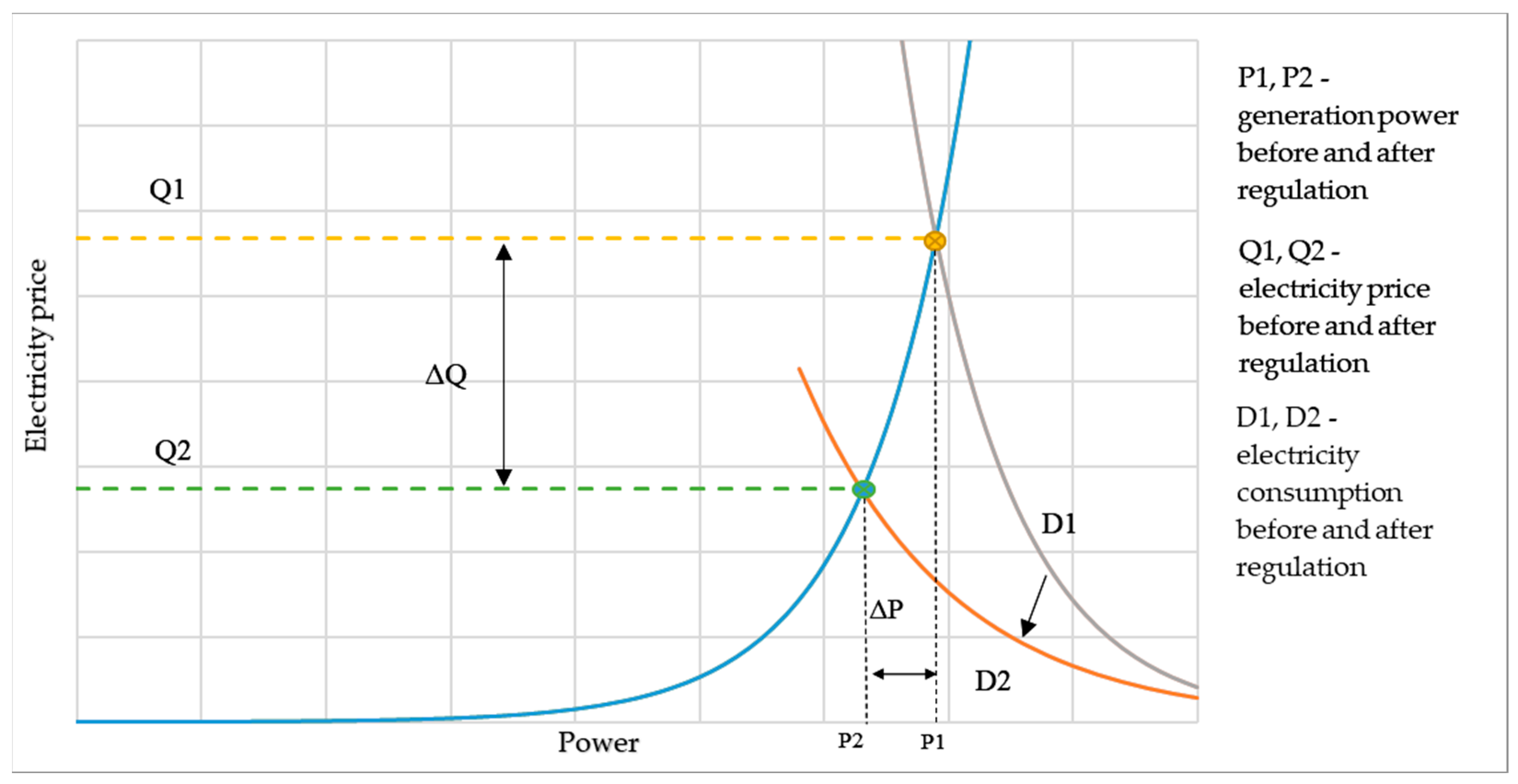
2.1. Electricity Cost Formation Mechanism
- Purchase price on the wholesale market (changes monthly);
- Tariff for electricity transmission services (set by the regulatory body of the subject of the federation, once a year);
- Sales markup of the supplier of last resort (set by the regulatory body of the constituent entity of the federation, as a rule, changes once a year);
- Payment for the services of infrastructure organizations (system and commercial operator of the unified electric power system).
2.2. Demand Response
2.3. Peak Shift Methods for Enterprises
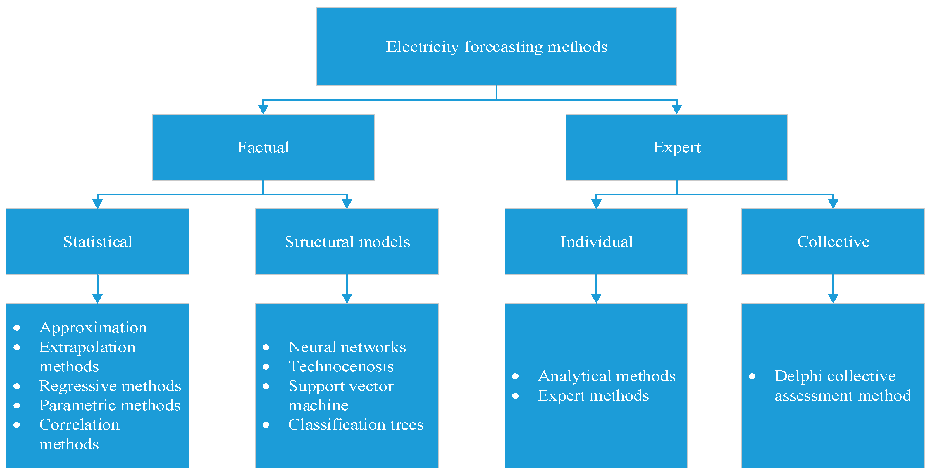
2.4. Machine Learning for Electrical Loads Forecasting
- Operational forecasting. Produced for participants in the wholesale electricity market with a lead time of 15 to 60 min.
- Short-term forecasting. Lead from an hour to a week ahead.
- Medium-term forecasting. From a week to a year in advance.
- Long-term forecasting. From a year to 20 years in advance. Long-term forecasting is often used for setting tariffs for population and economic development planning.
- -
- Ensemble training takes a lot of time and is not suitable for operational forecasting.
- -
- The selection of models for ensemble forecasting is very time consuming and an error in choosing a model can lead to a deterioration in the forecast.
- -
- When combining predictive algorithms, the ability to interpret the forecast results decreases, since for each algorithm the training features have a different weight.
3. Results
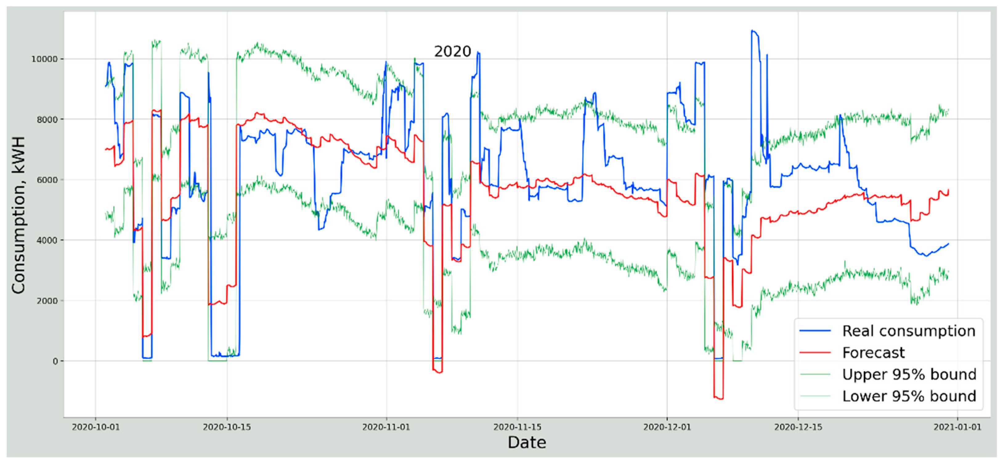
3.1. Forecasting the Electrical Loads of the Compressor Gas Compressor Station in Order to Improve the Efficiency of Demand Response, Taking into Account the Use of Energy Storage Systems
- Depth of study: 854 days (2.3 years).
- Forecast horizon: 120 days (~ 4 months).
- Values: hourly load.
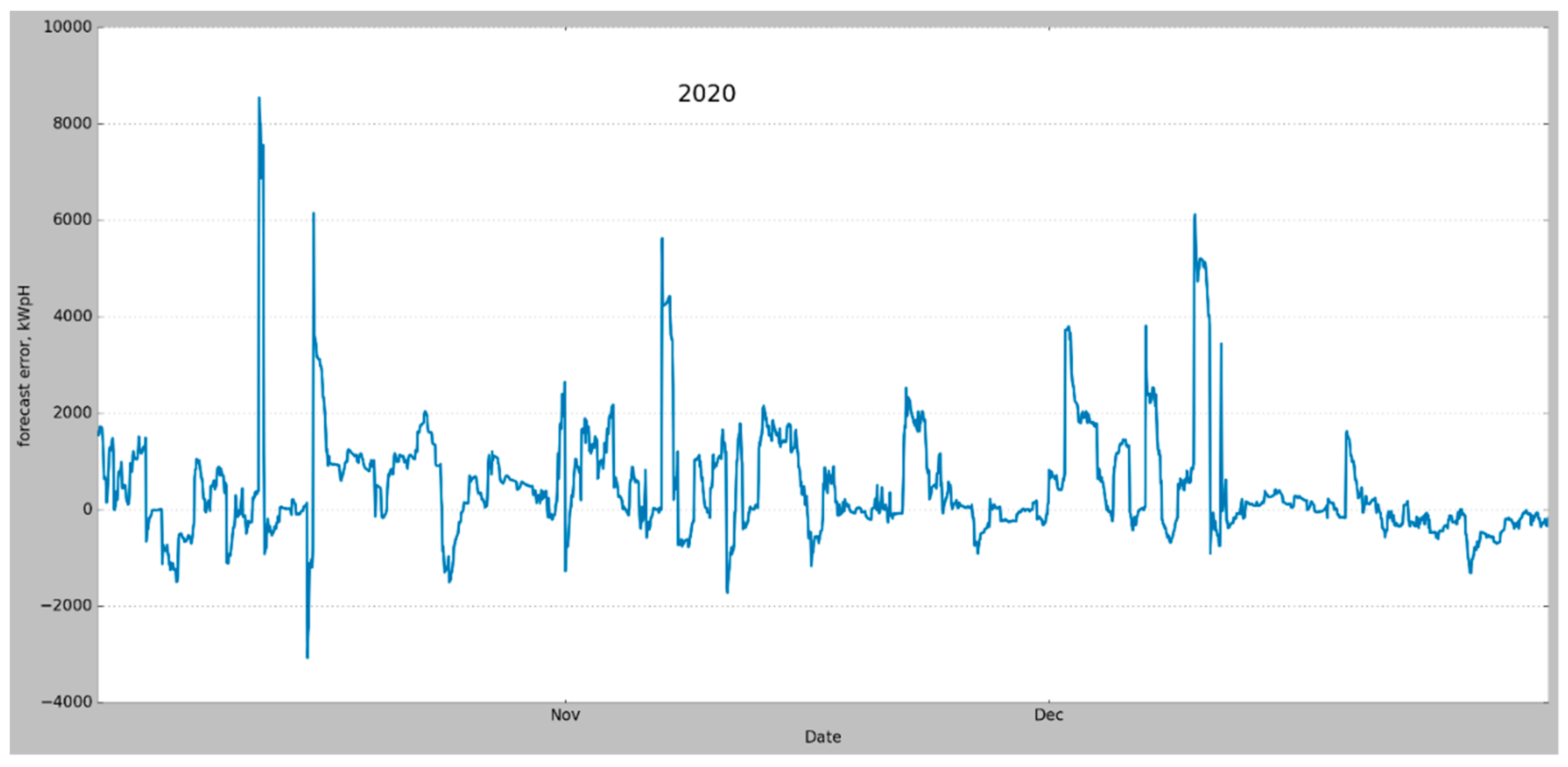
- Forecast score metric: mean absolute error.
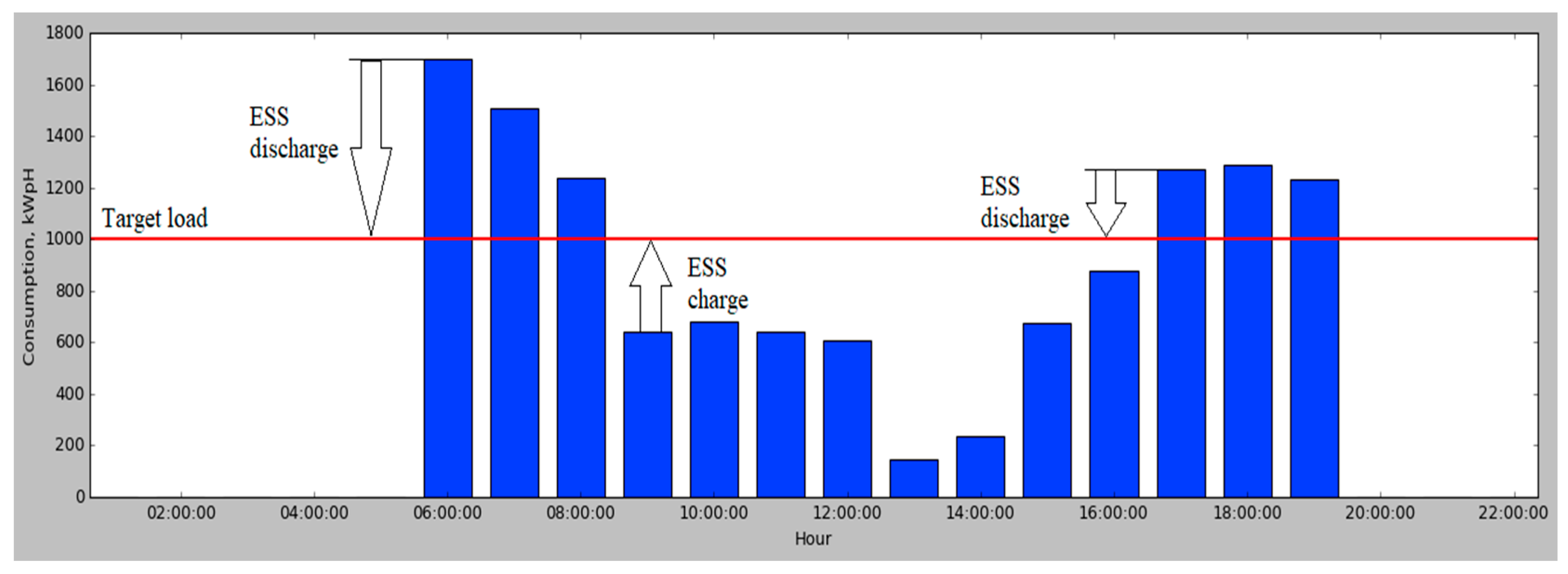
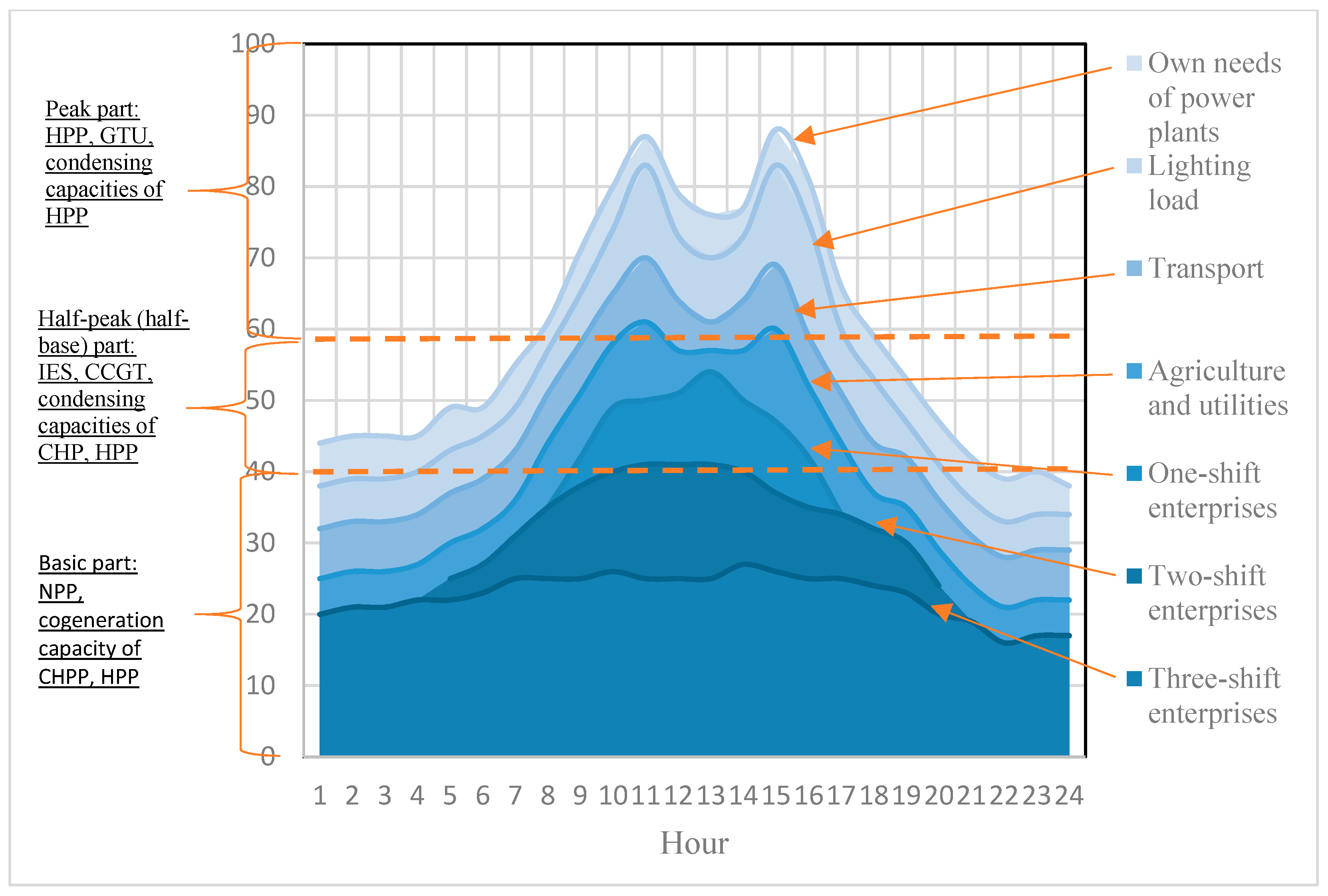
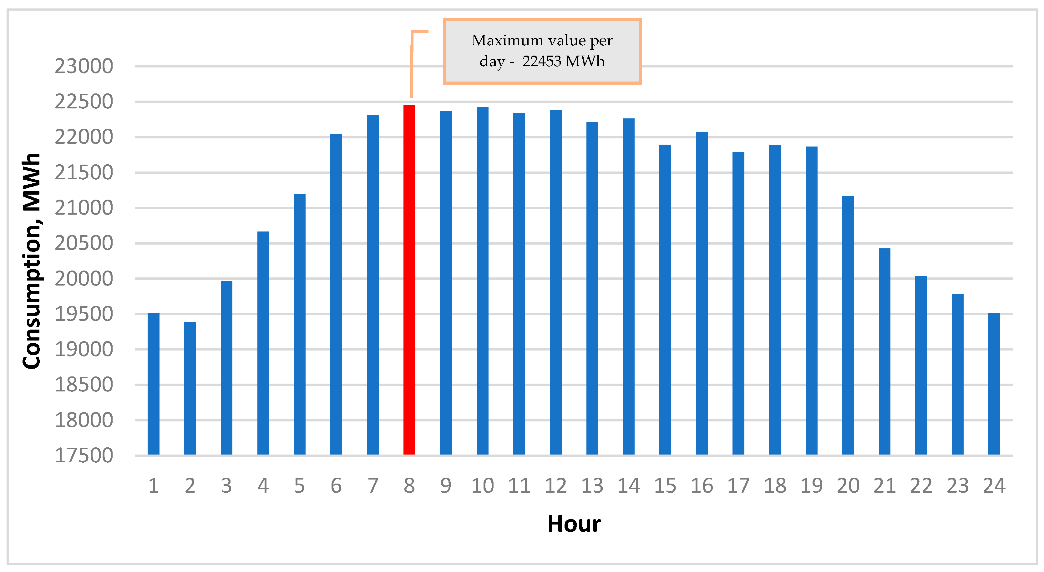
3.2. Regulation of the Electricity Load Schedule
- Changing the mode of production equipment.
- Changing the operating mode of air conditioning, heating and water supply systems.
- Using our own sources of small generation.
- Using rechargeable batteries to redistribute consumption peaks.
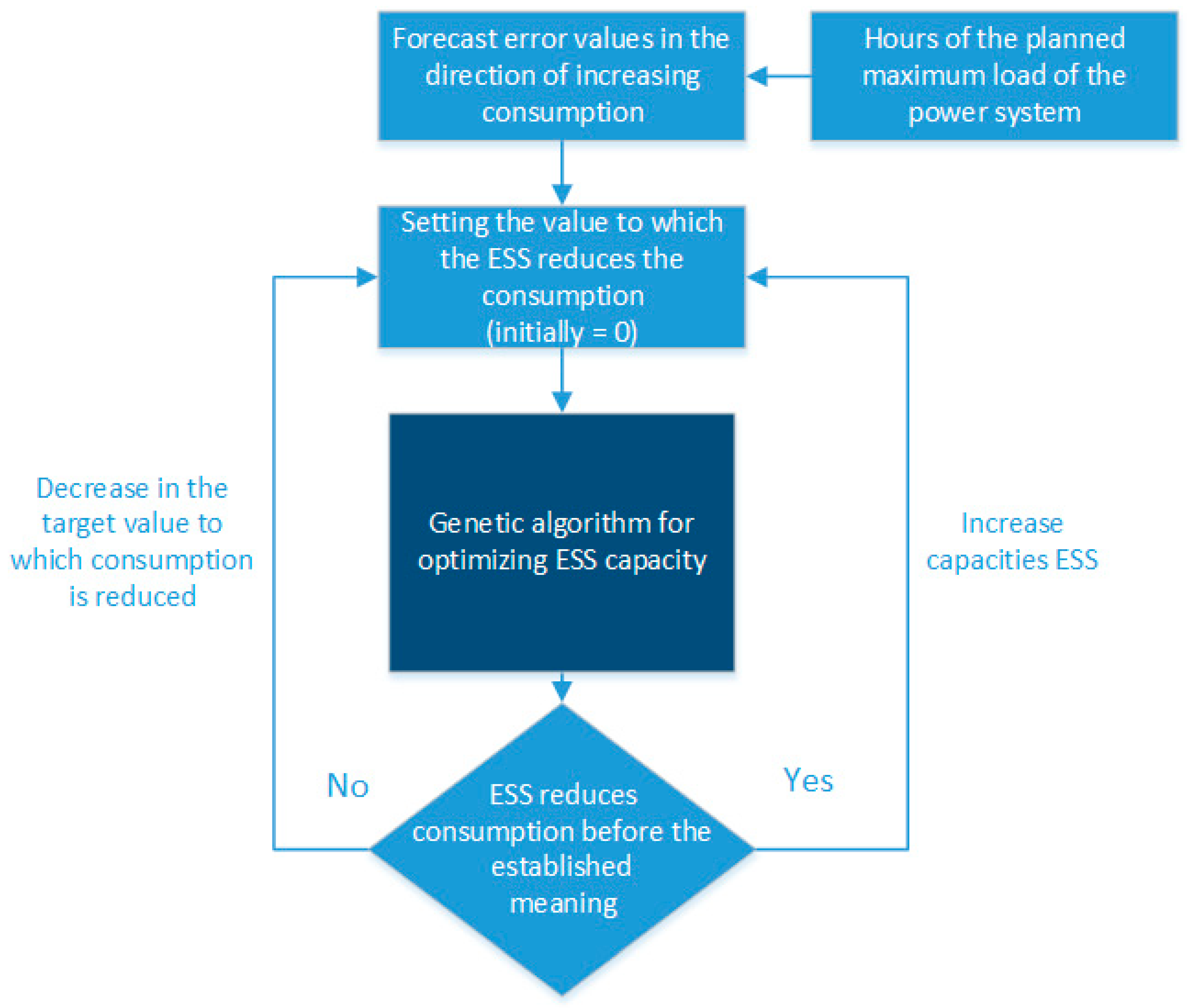
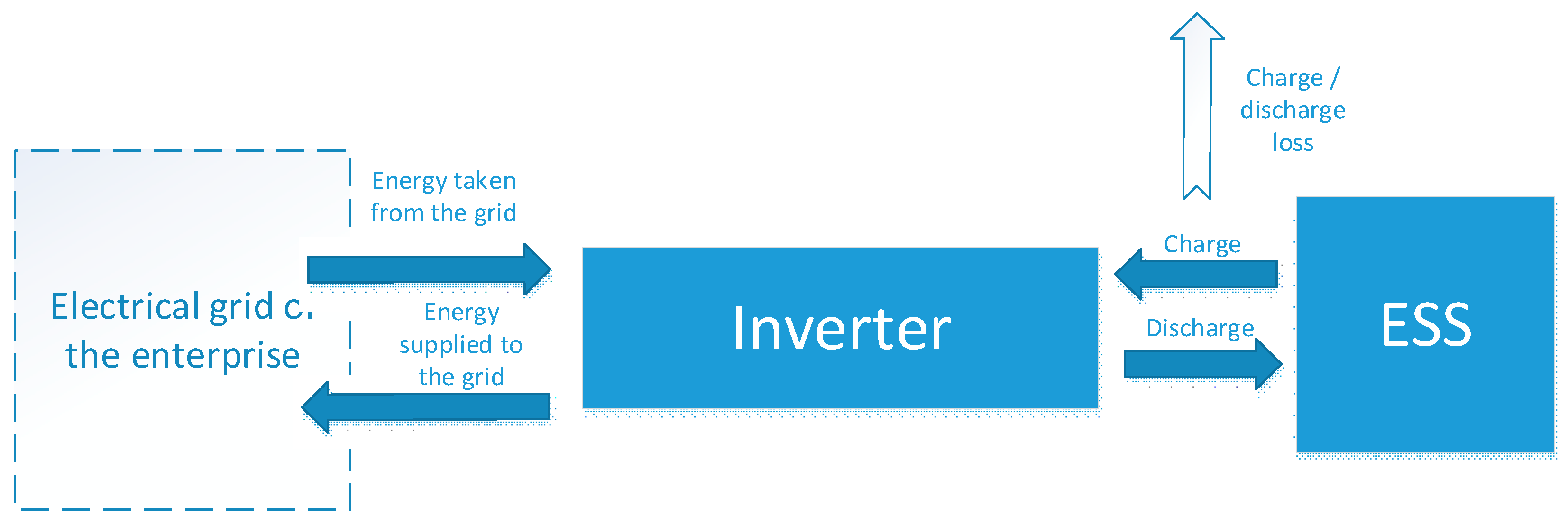
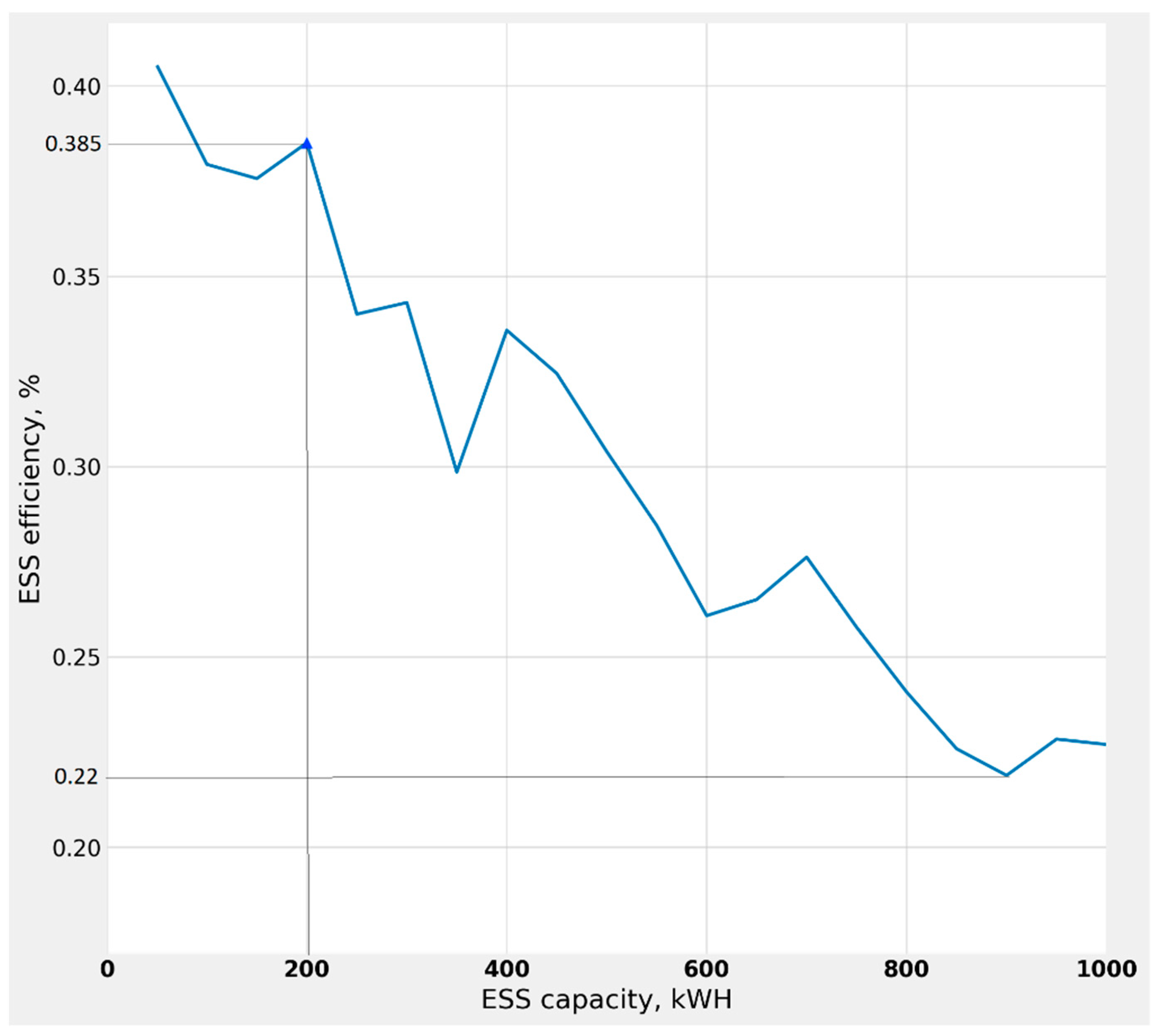
3.3. Using Energy Storage Systems to Improve the Efficiency of Power Supply
- The optimal effective capacity of ESS—200 kW.
- Average reduction in power consumption—77 kW.
- Efficiency of ESS operation—38.5%.
4. Discussion
- Direct reduction in deviations of actual electricity consumption from the declared plan;
- Participation in the demand response system;
- The use of energy storage devices to ensure the required voltage quality;
- Ensuring the reliability of power supply to especially critical categories of consumers.
5. Conclusions
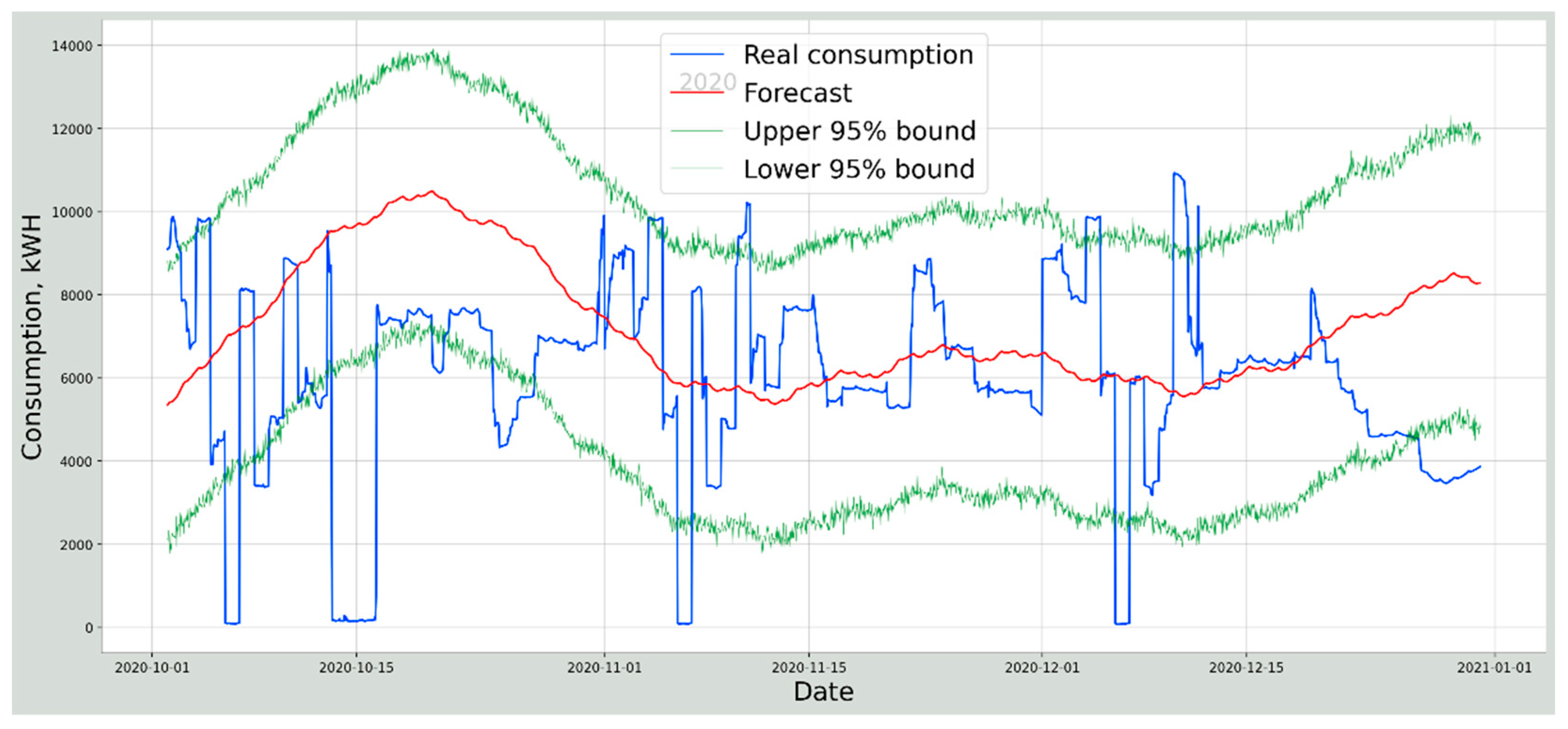
- The drawbacks of forecasting using autoregressive and statistical models for the power consumption graph with a high coefficient of unevenness were revealed.
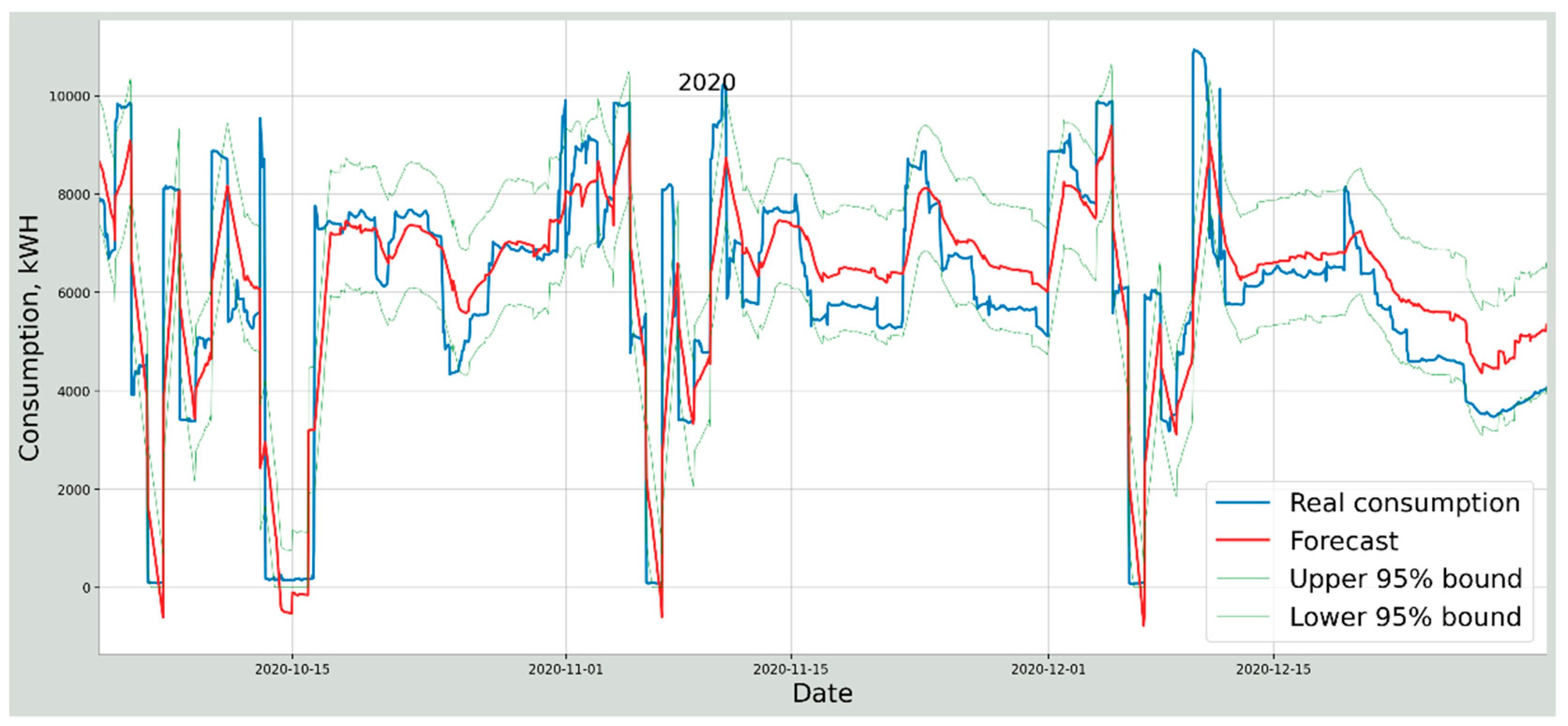
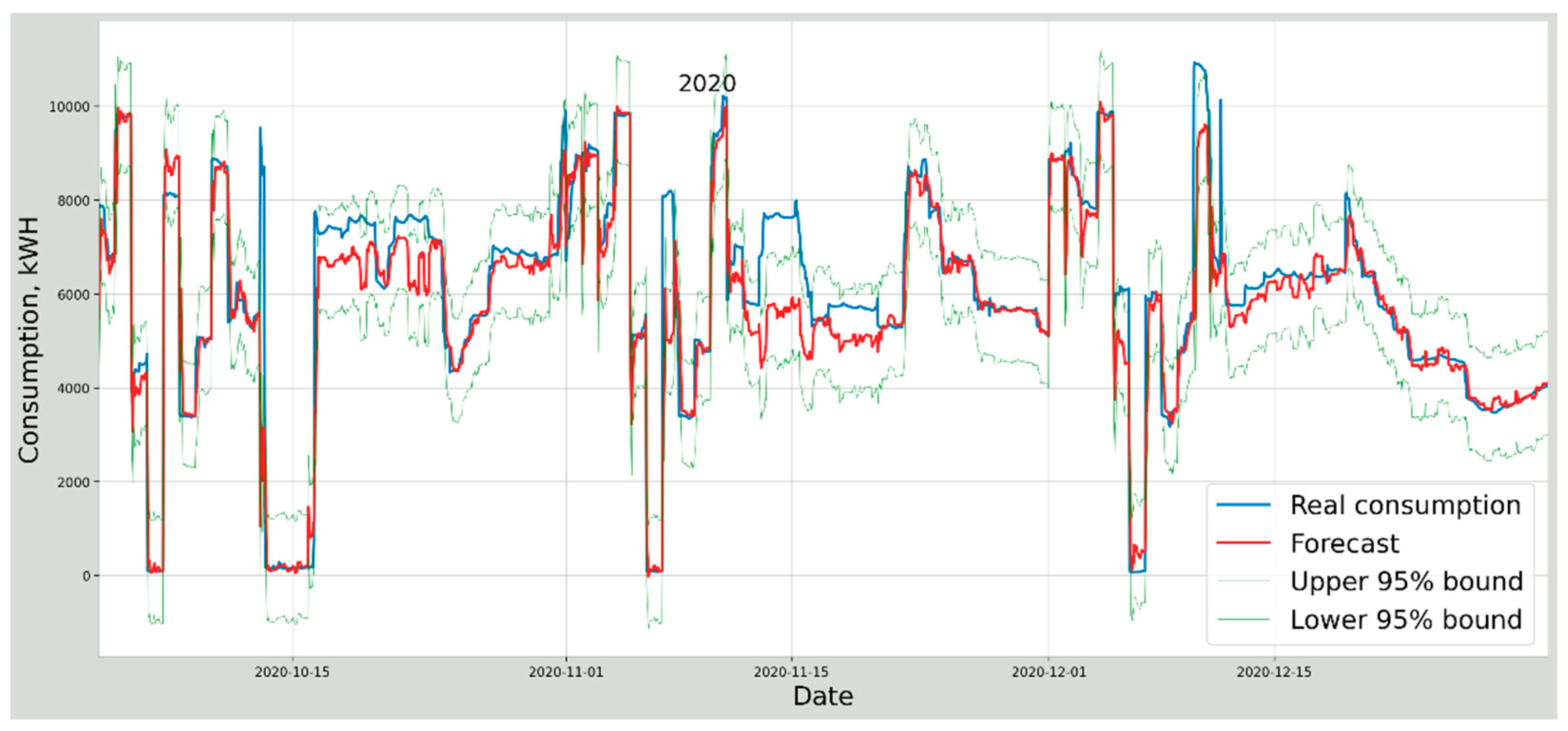
- Long-term forecasting based on decision trees using exogenous parameters and gradient boosting to find solutions with a high coefficient of unevenness of the load graph allowed to reduce the forecast error by four times over a forecast horizon of 3 months.
- The algorithm for choosing the optimal capacity of ESS allowed to achieve an increase in the efficiency of using the storage devices by almost two times, which would significantly reduce the capital costs of ESS installation.
Author Contributions
Funding
Data Availability Statement
Conflicts of Interest
Abbreviations
| ESS | energy storage system |
| RES | renewable energy sources |
| NSIBA | nondominated sorting bat algorithm |
| NPP | nuclear power plants |
| HPP | heat power plants |
| CHP | combined heat and power plants |
| DR | demand response |
| TPP | thermal power plants |
| GPU | gas pumping unit |
| FACTS | flexible alternative current transmission systems |
| DC | direct current |
| LSTM | long short-term memory |
| PICP | prediction interval coverage probability |
| ARIMA | autoregressive integrated moving average |
| MAE | mean absolute error |
References
- Song, C.H. Exploring and Predicting the Knowledge Development in the Field of Energy Storage: Evidence from the Emerging Startup Landscape. Energies 2021, 14, 5822. [Google Scholar] [CrossRef]
- What the Duck Curve Tells Us About Managing a Green Grid, California Independent System Operator. 2013. Available online: Large.stanford.edu/courses/2015/ph240/burnett2/docs/flexible.pdf (accessed on 27 October 2021).
- Hou, Q.; Zhang, N.; Du, E.; Miao, M.; Peng, F.; Kang, C. Probabilistic duck curve in high PV penetration power system: Concept, modeling, and empirical analysis in China. Appl. Energy 2019, 242, 205–215. [Google Scholar] [CrossRef]
- Nevzorova, T.; Kutcherov, V. The Role of Advocacy Coalitions in Shaping the Technological Innovation Systems: The Case of the Russian Renewable Energy Policy. Energies 2021, 14, 6941. [Google Scholar] [CrossRef]
- Yang, Y.; Lian, C.; Ma, C.; Zhang, Y. Research on Energy Storage Optimization for Large-Scale PV Power Stations under Given Long-Distance Delivery Mode. Energies 2020, 13, 27. [Google Scholar] [CrossRef] [Green Version]
- Alipour, M.; Stewart, R.A.; Sahin, O. Beyond the Diffusion of Residential Solar Photovoltaic Systems at Scale: Allegorising the Battery Energy Storage Adoption Behaviour. Energies 2021, 14, 5015. [Google Scholar] [CrossRef]
- Torabi, R.; Gomes, A.; Morgado-Dias, F. The Duck Curve Characteristic and Storage Requirements for Greening the Island of Porto Santo. In Proceedings of the 2018 Energy and Sustainability for Small Developing Economies (ES2DE), Funchal, Portugal, 9–12 July 2018; pp. 1–7. [Google Scholar] [CrossRef]
- Gajewski, P.; Pieńkowski, K. Control of the Hybrid Renewable Energy System with Wind Turbine, Photovoltaic Panels and Battery Energy Storage. Energies 2021, 14, 1595. [Google Scholar] [CrossRef]
- Qie, X.; Zhang, R.; Hu, Y.; Sun, X.; Chen, X. A Multi-Criteria Decision-Making Approach for Energy Storage Technology Selection Based on Demand. Energies 2021, 14, 6592. [Google Scholar] [CrossRef]
- Klaas, A.-K.; Beck, H.-P. A MILP Model for Revenue Optimization of a Compressed Air Energy Storage Plant with Electrolysis. Energies 2021, 14, 6803. [Google Scholar] [CrossRef]
- Mongird, K.; Viswanathan, V.; Balducci, P.; Alam, J.; Fotedar, V.; Koritarov, V.; Hadjerioua, B. An Evaluation of Energy Storage Cost and Performance Characteristics. Energies 2020, 13, 3307. [Google Scholar] [CrossRef]
- Chowdhury, N.; Pilo, F.; Pisano, G. Optimal Energy Storage System Positioning and Sizing with Robust Optimization. Energies 2020, 13, 512. [Google Scholar] [CrossRef] [Green Version]
- Szott, M.; Jarnut, M.; Kaniewski, J.; Pilimon, Ł.; Wermiński, S. Fault-Tolerant Control in a Peak-Power Reduction System of a Traction Substation with Multi-String Battery Energy Storage System. Energies 2021, 14, 4565. [Google Scholar] [CrossRef]
- Sun, T.; Zeng, L.; Zheng, F.; Zhang, P.; Xiang, X.; Chen, Y. Two-Layer Optimization Model for the Siting and Sizing of Energy Storage Systems in Distribution Networks. Processes 2020, 8, 559. [Google Scholar] [CrossRef]
- Yun, P.; Ren, Y.; Xue, Y. Energy-Storage Optimization Strategy for Reducing Wind Power Fluctuation via Markov Prediction and PSO Method. Energies 2018, 11, 3393. [Google Scholar] [CrossRef] [Green Version]
- Wang, Z.; Negash, A.; Kirschen, D.S. Optimal scheduling of energy storage under forecast uncertainties. IET Gener. Transm. Distrib. 2017, 11, 4220–4226. [Google Scholar] [CrossRef]
- Han, K.B.; Jung, J.; Kang, B.O. Real-Time Load Variability Control Using Energy Storage System for Demand-Side Management in South Korea. Energies 2021, 14, 6292. [Google Scholar] [CrossRef]
- Ivanchenko, O.S. Sustainable development of the organization. Eur. Sci. 2016, 11, 44–47. [Google Scholar]
- Lebedev, V.; Rubanov, I.; Sivakov, D. Est’ u reformy nachalo, net u reformy kontsa. Ekspert 2012, 20, 16–22. Available online: https://expert.ru/expert/2012/20/est-u-reformyi-nachalo-net-u-reformyi-kontsa/ (accessed on 27 October 2021).
- Electricity: Time to Cut Costs. Energy Bulletin of the Analytical Center under the Government of the Russian Federation. 2016. Available online: http://ac.gov.ru/files/publication/a/9764.pdf (accessed on 27 October 2021).
- Cost of Electricity by Source. Available online: https://ru.abcdef.wiki/wiki/Cost_of_electricity_by_source (accessed on 27 October 2021).
- Sidorovskaya, N. Demand Management in the World Electricity Markets. Pro. J. 2015, 7, 28–34. [Google Scholar]
- Rudakov, A.D. Evaluating the efficiency of energy management using demand response technology in Russia. Scythian 2020, 44, 329–333. [Google Scholar]
- Tellidou, A.C.; Bakirtzis, A. Agent-Based Analysis of Capacity Withholding and Tacit Collusion in Electricity Markets. IEEE Trans. Power Syst. 2007, 22, 1735–1742. [Google Scholar] [CrossRef]
- Albadi, M.H.; El-Saadany, E.F. Demand Response in Electricity Markets: An Overview. In Proceedings of the 2007 IEEE Power Engineering Society General Meeting, Tampa, FL, USA, 24–28 July 2007; pp. 1–5. [Google Scholar] [CrossRef]
- Kirschen, D.S. Demand-side view of electricity markets. IEEE Trans. Power Syst. 2003, 18, 520–527. [Google Scholar] [CrossRef] [Green Version]
- Bayer, B. Demand Response—Is the USA a Role Model for Germany? Analysis of the Integration of Demand Response into the American Capacity and Balancing Markets—IASS Working Paper. 2014. Available online: https://publications.iass-potsdam.de/pubman/faces/ViewItemOverviewPage.jsp?itemId=item_1157897 (accessed on 27 October 2021).
- Cai, Y.; Liu, Y.; Tang, X.; Tan, Y.; Cao, Y. Increasing Renewable Energy Consumption Coordination with the Monthly Interprovincial Transaction Market. Front. Energy Res. 2021, 9, 355. [Google Scholar] [CrossRef]
- Bovera, F.; Delfanti, M.; Bellifemine, F. Economic opportunities for Demand Response by Data Centers within the new Italian Ancillary Service Market. In Proceedings of the 2018 IEEE International Telecommunications Energy Conference (INTELEC), Turino, Italy, 7–11 October 2018; pp. 1–8. [Google Scholar] [CrossRef] [Green Version]
- Gorshkov, A.S.; Vatin, N.I.; Rymkevich, P.P.; Kydrevich, O.O. Payback period of investments in energy saving. Mag. Civ. Eng. 2018, 78, 65–75. [Google Scholar] [CrossRef]
- Turysheva, A.; Voytyuk, I.; Guerra, D. Estimation of Electricity Generation by an Electro-Technical Complex with Photoelectric Panels Using Statistical Methods. Symmetry 2021, 13, 1278. [Google Scholar] [CrossRef]
- The Government of the Russian Federation No. 699 dated July 20 2016 On Amendments to the Rules of the Wholesale Electricity and Power Market, Approved by the Resolution of the Government of the Russian Federation No. 1172 dated December 27, 2011. Available online: http://government.ru/docs/23954/ (accessed on 27 October 2021).
- JSC System Operator of the Unified Energy System (JSC SO UES). The Concept of Functioning of Aggregators of Distributed Energy Resources as Part of the Unified Energy System of Russia. Electricity Demand Management Aggregators. Available online: https://www.so-ups.ru/fileadmin/files/company/markets/dr/docs/dr_agregator_concept.pdf (accessed on 27 October 2021).
- Dzyuba, A.P.; Solovyova, I.A. Model of price-dependent management of an industrial enterprise energy consumption. SHS Web Conf. 2017, 35, 6. [Google Scholar]
- Main Characteristics of the Russian Electric Power Industry. Available online: https://minenergo.gov.ru/node/532 (accessed on 27 October 2021).
- Shklyarskiy, Y.E.; Skamyin, A.N.; Shklyarskiy, A.Y. Effect of higher harmonics on electric power metering in a steel maker’s power networks. Tsvetnye Met. 2020, 10, 64–69. [Google Scholar] [CrossRef]
- Voronin, V.; Nepsha, F. Simulation of the electric drive of the shearer to assess the energy efficiency indicators of the power supply system. J. Min. Inst. 2021, 246, 633–639. [Google Scholar] [CrossRef]
- Abramovich, B.N.; Veprikov, A.A.; Sychev, Y.A.; Lyakh, D.A. Use of active power transducers in industrial DC power systems supplying electrolysis cells. Tsvetnye Met. 2020, 2, 95–100. [Google Scholar] [CrossRef]
- Schipachev, A.; Dmitrieva, A. Application of the resonant energy separation effect at natural gas reduction points in order to improve the energy efficiency of the gas distribution system. J. Min. Inst. 2021, 248, 253–259. [Google Scholar] [CrossRef]
- Abramovich, B.N.; Babanova, I.S. Development of neural network models to predict and control power consumption in mineral mining industry. Min. Inf. Anal. Bull. 2018, 5, 206–213. [Google Scholar] [CrossRef]
- Solovieva, I.A. Price-Dependent Management of Costs for Electricity Consumption at Industrial Enterprises: Abstract of Thesis. Doctors of Economic Sciences. Chelyabinsk. 2018. Available online: https://www.susu.ru/ru/dissertation/d-21229807/soloveva-irina-aleksandrovna (accessed on 27 October 2021).
- Ungureanu, S.; Topa, V.; Cziker, A.C. Analysis for Non-Residential Short-Term Load Forecasting Using Machine Learning and Statistical Methods with Financial Impact on the Power Market. Energies 2021, 14, 6966. [Google Scholar] [CrossRef]
- Bouktif, S.; Fiaz, A.; Ouni, A.; Serhani, M.A. Optimal Deep Learning LSTM Model for Electric Load Forecasting using Feature Selection and Genetic Algorithm: Comparison with Machine Learning Approaches †. Energies 2018, 11, 1636. [Google Scholar] [CrossRef] [Green Version]
- Wang, Y.; Chen, J.; Chen, X.; Zeng, X.; Kong, Y.; Sun, S.; Guo, Y.; Liu, Y. Short-Term Load Forecasting for Industrial Customers Based on TCN-LightGBM. IEEE Trans. Power Syst. 2021, 36, 1984–1997. [Google Scholar] [CrossRef]
- Eeeguide. Forecasting Methodology. 2014. Available online: http://www.eeeguide.com/forecasting-methodology/ (accessed on 27 October 2021).
- Bogomolov, A.; Lepri, B.; Larcher, R.; Antonelli, F.; Pianesi, F.; Pentland, A. Energy consumption prediction using people dynamics derived from cellular network data. EPJ Data Sci. 2016, 5, 1. [Google Scholar] [CrossRef] [Green Version]
- Kang, T.; Lim, D.Y.; Tayara, H.; Chong, K.T. Forecasting of Power Demands Using Deep Learning. Appl. Sci. 2020, 10, 7241. [Google Scholar] [CrossRef]
- Cho, H.; Goude, Y.; Brossat, X.; Yao, Q. Modelling and Forecasting Daily Electricity Load via Curve Linear Regression. In Modeling and Stochastic Learning for Forecasting in High Dimensions; Antoniadis, A., Poggi, J.M., Brossat, X., Eds.; Lecture Notes in Statistics; Springer: Cham, Switzerland, 2015; Volume 217. [Google Scholar] [CrossRef] [Green Version]
- Zhukovskiy, Y.L.; Batueva, D.E.; Buldysko, A.D.; Gil, B.; Starshaia, V.V. Fossil Energy in the Framework of Sustainable Development: Analysis of Prospects and Development of Forecast Scenarios. Energies 2021, 14, 5268. [Google Scholar] [CrossRef]
- Roccazzella, F.; Gambetti, P.; Vrins, F. Optimal and Robust Combination of Forecasts via Constrained Optimization and shrinkage. Int. J. Forecast. 2021. Available online: https://www.sciencedirect.com/science/article/pii/S0169207021000650 (accessed on 27 October 2021). [CrossRef]
- Taylor, S.J.; Letham, B. Forecasting at scale. Peer J. Preprints 2017, 5, e3190v2. [Google Scholar] [CrossRef]
- Zuniga-Garcia, M.A.; Santamaría-Bonfil, G.; Arroyo-Figueroa, G.; Batres, R. Prediction Interval Adjustment for Load-Forecasting using Machine Learning. Appl. Sci. 2019, 9, 5269. [Google Scholar] [CrossRef] [Green Version]
- Su, D.; Ting, Y.Y.; Ansel, J. Tight Prediction Intervals Using Expanded Interval Minimization. 2018. Available online: https://arxiv.org/abs/1806.11222 (accessed on 27 October 2021).
- Critical Values of the Student′s-t Distribution. NIST/SEMATECH e-Handbook of Statistical Methods. Available online: https://itl.nist.gov/div898/handbook/eda/section3/eda3672.htm (accessed on 27 October 2021).
- Hastie, T.; Tibshirani, R. Generalized Additive Models: Some Applications. J. Am. Stat. Assoc. 1987, 82, 371–386. [Google Scholar] [CrossRef]
- Ke, G.; Meng, Q.; Finley, T.; Wang, T.; Chen, W.; Ma, W.; Ye, Q.; Liu, T.-Y. LightGBM: A Highly Efficient Gradient Boosting Decision Tree. Adv. Neural Inf. Process. Syst. 2017, 30, 3146–3154. [Google Scholar]
- Rahmann, C.; Chamas, S.I.; Alvarez, R.; Chavez, H.; Ortiz-Villalba, D.; Shklyarskiy, Y. Methodological Approach for Defining Frequency Related Grid Requirements in Low-Carbon Power Systems. IEEE Access 2020, 8, 161929–161942. [Google Scholar] [CrossRef]
- Van der Veen, R.A.; Hakvoort, R.A. The Electricity Balancing Market: Exploring the Design Challenge. 2016. Available online: https://www.journals.elsevier.com/utilities-policy (accessed on 27 October 2021).
- Website of the System Operator of the Russian Federation. Available online: https://www.so-ups.ru/ (accessed on 27 October 2021).
- Appendix No. 12 to the Agreement on Joining the Wholesale Market Trading System. Regulation for Determining the Scope, Initiatives and Cost of Deviations. Approved July 14 2006. Available online: https://www.np-sr.ru/sites/default/files/sr_regulation/reglaments/r12_01072020_22062020.pdf (accessed on 27 October 2021).
- Cho, S.-M.; Yun, S.-Y. Optimal Power Assignment of Energy Storage Systems to Improve the Energy Storage Efficiency for Frequency Regulation. Energies 2017, 10, 2092. [Google Scholar] [CrossRef] [Green Version]
- Silva-Saravia, H.; Pulgar-Painemal, H.; Mauricio, J.M. Flywheel Energy Storage Model, Control and Location for Improving Stability: The Chilean Case. IEEE Trans. Power Syst. 2017, 32, 3111–3119. [Google Scholar] [CrossRef]
- Carrizosa, M.J.; Stankovic, N.; Vannier, J.-C.; Shklyarskiy, Y.E.; Bardanov, A.I. Multi-terminal dc grid overall control with modular multilevel converters. J. Min. Inst. 2020, 243, 357. [Google Scholar] [CrossRef]
- Papadopoulos, V.; Knockaert, J.; Develder, C.; Desmet, J. Peak Shaving through Battery Storage for Low-Voltage Enterprises with Peak Demand Pricing. Energies 2020, 13, 1183. [Google Scholar] [CrossRef] [Green Version]
- Skamyin, A.N.; Vasilkov, O.S.; Belsky, A.A. The use of hybrid energy storage devices for balancing the electricity load profile of enterprises. Energ. Proc. CIS High. Educ. Inst. Power Eng. Assoc. 2020, 3, 212–222. [Google Scholar] [CrossRef]
- Hesse, H.C.; Schimpe, M.; Kucevic, D.; Jossen, A. Lithium-Ion Battery Storage for the Grid—A Review of Stationary Battery Storage System Design Tailored for Applications in Modern Power Grids. Energies 2017, 10, 2107. [Google Scholar] [CrossRef] [Green Version]


| Parameter | Value |
|---|---|
| Average load, MW | 5206.80 |
| RMS load, MW | 6077.37 |
| Form Factor | 1.17 |
| Maximum load, MW | 11,937.62 |
| Minimum load, MW | 0.00 |
| Max ratio | 2.29 |
| Chart fill factor | 0.44 |
| The coefficient of unevenness of the daily load schedule | 0.86 |
| The coefficient of unevenness of the weekly load schedule | 0.36 |
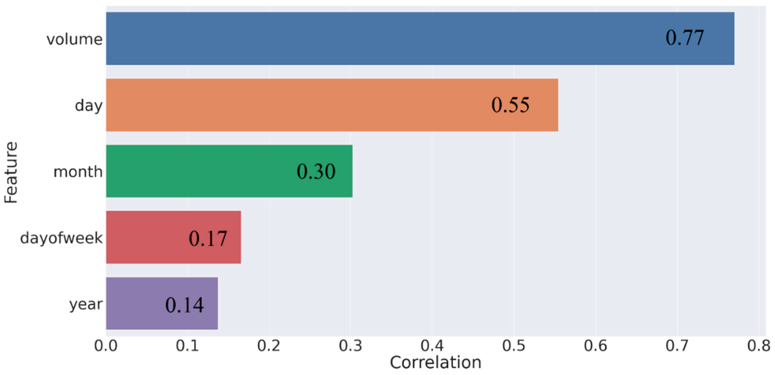
| Parameter | Production Volume | Year | Month | Day | Day of Week | Hour |
|---|---|---|---|---|---|---|
| Correlation | 0.77 | 0.16 | 0.11 | 0.15 | 0.05 | 0.05 |
| Model | Mean Absolute Error, kWh | Root Mean Squared Error, kWh | Mean Absolute Percentage Error, % | Forecast Interval Width, % |
|---|---|---|---|---|
| Autoregressive model | 2104 | 3119 | 40 | 64.4 |
| Autoregressive model with exogenous factors | 1324 | 1806 | 25 | 41.2 |
| Linear regression | 962 | 1070 | 18 | 20.8 |
| Regression with gradient boosting | 521 | 758 | 10 | 18.4 |
| Object | Parameter |
|---|---|
| Effective power of ESS, kWh | 200 |
| Average cost of electricity, USD/kW * h | 0.046 1 |
| Duration of load reduction with demand control, hour | 4 |
| Payment for participation in the demand response system, USD/kWh | 7.15 1 |
| Month | Effect of Reducing Deviations, USD | Effect of Participation in Demand Response, USD | Result Effect, USD | Relative Reduction in Electricity Bills, % |
|---|---|---|---|---|
| 1 | 106.53 | 357.53 | 464.07 | 0.25 |
| 2 | 142.62 | 357.53 | 500.15 | 0.24 |
| 3 | 116.11 | 357.53 | 473.65 | 0.27 |
| 4 | 86.53 | 357.53 | 444.06 | 0.15 |
| 5 | 77.44 | 357.53 | 434.98 | 0.23 |
| 6 | 129.14 | 357.53 | 486.68 | 0.53 |
| 7 | 194.45 | 357.53 | 551.98 | 0.29 |
| 8 | 187.80 | 357.53 | 545.34 | 0.42 |
| 9 | 253.51 | 357.53 | 611.04 | 0.31 |
| 10 | 164.31 | 357.53 | 521.84 | 0.25 |
| 11 | 212.42 | 357.53 | 569.95 | 0.27 |
| 12 | 244.30 | 357.53 | 601.84 | 0.29 |
| Total | 1915.17 | 4290.41 | 6205.58 | 0.27 |
Publisher’s Note: MDPI stays neutral with regard to jurisdictional claims in published maps and institutional affiliations. |
© 2021 by the authors. Licensee MDPI, Basel, Switzerland. This article is an open access article distributed under the terms and conditions of the Creative Commons Attribution (CC BY) license (https://creativecommons.org/licenses/by/4.0/).
Share and Cite
Senchilo, N.D.; Ustinov, D.A. Method for Determining the Optimal Capacity of Energy Storage Systems with a Long-Term Forecast of Power Consumption. Energies 2021, 14, 7098. https://doi.org/10.3390/en14217098
Senchilo ND, Ustinov DA. Method for Determining the Optimal Capacity of Energy Storage Systems with a Long-Term Forecast of Power Consumption. Energies. 2021; 14(21):7098. https://doi.org/10.3390/en14217098
Chicago/Turabian StyleSenchilo, Nikita Dmitrievich, and Denis Anatolievich Ustinov. 2021. "Method for Determining the Optimal Capacity of Energy Storage Systems with a Long-Term Forecast of Power Consumption" Energies 14, no. 21: 7098. https://doi.org/10.3390/en14217098
APA StyleSenchilo, N. D., & Ustinov, D. A. (2021). Method for Determining the Optimal Capacity of Energy Storage Systems with a Long-Term Forecast of Power Consumption. Energies, 14(21), 7098. https://doi.org/10.3390/en14217098