Exergoeconomic Optimization of Polymeric Heat Exchangers for Geothermal Direct Applications

Abstract

The highest economic costs of a geothermal plant are basically related to well drilling and heat exchanger maintenance cost due to the chemical aggressiveness of geothermal fluid. The possibility to reduce these costs represents an opportunity to push toward geothermal plants development. Such challenges are even more important in the sites with a low-medium temperature geothermal fluids (90–120 °C) availability, where the use of these fluids for direct thermal uses can be very advantageous. For this reason, in this study, a direct geothermal heating system for a building will be investigated by considering a plastic plate heat exchanger. The choice of a polymeric heat exchanger for this application is upheld by its lower purchase cost and its higher fouling resistance than the common metal heat exchangers, overcoming the economic issues related to conventional geothermal plant. Thus, the plastic plate heat exchanger was, firstly, geometrical and thermodynamical modeled and, after, exergoeconomic optimized. In particular, an exergoeconomic analysis was assessed on the heat exchanger system by using a MATLAB and REFPROP environment, that allows for determination of the exergoeconomic costs of the geothermal fluid extraction, the heat exchanger, and the heating production. A sensitivity analysis was performed to evaluate the effect of main design variable (number of plates/channels) and thermodynamic variable (inlet temperature of geothermal fluid) on yearly exergoeconomic product cost. Then, the proposed methodology was applied to a case study in South of Italy, where a low-medium enthalpy geothermal potential exists. The plate-heat exchanger was used to meet the space heating requests of a single building by the exploitation of low-medium temperature geothermal fluids availability in the selected area. The results show that the inlet temperature of geothermal fluid influences the exergoeconomic cost more than the geometrical parameter. The variation of the exergoeconomic cost of heat exchanger with the inlet geothermal fluid temperature is higher than the change of the exergoeconomic costs associated to wells drilling and pumping with respect to the same variable. This is due the fact that, in the selected zone of South of Italy, it is possible to find geothermal fluid in the temperature range of 90–120 °C, at shallow depth. The product exergoeconomic cost is the lowest when the temperature is higher than 105 °C; thus, the smallest heat exchange area is required. The exergoeconomic optimization determines an optimum solution with a total product cost of 922 €/y for a temperature of geothermal fluid equal to 117 °C and with a number of plates equal to 15.

1. Introduction

Today, the ambitious energy and environmental European Union (EU) target is to limit global temperature increase below 2 °C. Among the different sectors involved in the decarbonization by 2050, such as transport, industry, civil, and agriculture, the building sector causes 36% of greenhouse gas (GHG) emissions, and it represents the pivotal sector to achieve the energy transition [1]. The highest share of energy demand in EU building sector has been caused by space heating in 2018; in fact, it covers 64% of energy building consumption in EU. Moreover, EU space heating requests are met 5% by electricity, 5% by solid fuel, 10% by derived heat, 4% by oil and petrol product, 23% by renewable and waste heat, and 43% by natural gas [2]. For these reasons, the EU promotes the replacement of fossil-fuel-based heating systems with renewable-based one in order to mitigate the building sector environmental impact. A massive use of renewable energy sources (RESs) to activate space heating system is a good strategy to obtain the EU targets. The renewable energy use for heating purposes in 2018 amounted to 2270 TJ of solar energy, 44,411 TJ of geothermal energy, 477,666 TJ of waste heat recovery, and 641,308 TJ of biofuels [3].

The use of RESs to meet the space heating needs could be significantly improved with the exploitation of RESs’ lowly weather influences, such as geothermal source. The geothermal energy is low dependent from weather conditions for its nature, and it presents a higher capacity factor than other RESs, such as solar or wind. The total installed geothermal capacity for direct use is increased by 52% from 2015 to 2019, reaching 107,727 MW_th. The increasing trend is caused by the Ground Source Heat Pumps use that do not draw the geothermal fluid from the ground. Instead, the geothermal use for direct space heating (single building and district heating system) increased by 68.0% in installed capacity, and 83.8% in annual energy use, from 2015 to 2019 [4]. However, a great potential for geothermal energy exploitation exists, but economic issues related to geothermal plant installation curb the exploitation of these technologies. Indeed, the high cost for drilling wells, and the great maintenance and purchase costs of metallic heat exchangers (HEXs) interacting with geothermal fluids, are the major cost items for geothermal plants.

The high HEXs′ maintenance costs are caused by the interaction between the aggressive geothermal fluid and the heat-transfer fluid leading fouling problems [5]. This fouling issue causes the worsening of two factors in the hydronic system for heating and cooling: the increase of friction pressure losses and the worsening of thermal heat transfer coefficient. The decrease of crossing flow section also determines the reduction of plant efficiency. For these reasons, the heat exchangers of the geothermal plants require the continuous cleaning maintenance and, sometimes, the periodic replacement of traditional steel component or the employment of high fouling resistant metals, such as titanium, causing the purchase cost increase.

During the last few years, the alternative materials for HEXs are introduced to solve the fouling problem in different aggressive environments for tube plate [6], tubular immersion [6], plate [7], shell and tube [8] heat exchangers, and also economizers [9]. The advantages of plastic materials are the lower costs and weights than metallic ones; high anti-corrosion and antifouling resistances that allow the interaction with chemical aggressive fluids and good mechanical properties [10]; sustainability of manufacturing process; and the possibility of different fields of applications, such as heat recovery systems, desiccant cooling systems, electronic devices cooling, water desalination systems, and cooling evaporators [11]. Nevertheless, the polymers are characterized by low atomic density and low thermal conductivity (0.1 ÷ 0.3 W/m·K); for this reason, their employments need geometric and thermodynamic optimization. Ceglia et al. [12] considered the employment of plastic material in shell and tube heat exchangers as a replacement of traditional metals one to overcome the fouling issue caused by aggressive geothermal fluid in a cogeneration system. The results showed the reduction of HEX purchase cost up to 73% by replacing titanium with high density polymers [13], and the maximum excess of heat exchange surface area was equal to 47%. The plastic HEX models optimization, aimed to match the economic advantages and the improving of heat transfer, represents a pivotal strategy to push toward the increase of geothermal source exploitation.

In this context, the thermoeconomic optimization by using exergy analysis is considered a good approach to evaluate the economic and thermodynamic advantages of a thermal system by combining the quality and the quantity of energy with its economic value. This approach is so called exergoeconomic analysis. Thus, the exergoeconomic analysis of geothermal-based systems is spreading, demonstrating that it is useful for the identification of the thermodynamic inefficiencies in such systems. Luo et al. [14] have carried out an exergy analysis on an integrated cascade utilization system of geothermal water to identify the optimal temperature scheme. Arslan et al. [15] have used the exergoeconomic analysis to investigate a heating network for an integrated geothermal system in Turkey. To define the most performed solution for different pipelines dimension, the variation of total cost based on diameter of the pipes has been analyzed. The outcomes show that the change of the outlet temperature of geothermal fluid has a negligible effect on the optimum point. Different researchers have paid attention on exergoeconomic analysis of heat exchangers in geothermal applications to minimize the capital cost and investment cost of components by using multiple algorithms and methodologies. Jamil et al. [16] have defined an exergoeconomic optimization by considering design and operating parameters and also fiscal parameters for a shell and tube heat exchanger. The results show that the increase of mass flow rate and the baffles increased the operating cost because of an exponential growth in the pressure drops. Finally, the optimization reduced the heat transfer area by 26.4%, capital cost by 20%, and operational cost by 50%. Hajabdollahi et al. [17] have presented a study of optimization for gasket-plate and shell and tube heat exchangers. The aim of study is the minimization of the capital and operating costs by using decision variables. The results in the case of gasket-plate show an improvement of 13% in the total cost compared with shell and tube heat exchangers with the same operating conditions. In addition, the total cost in plate configuration decreases by increase of plate number. Instead, for shell and tube heat exchangers, the operating cost increases by the growth of both cold and hot side mass flow rates due to the increase of Reynolds number and consequently pressure drops. In Reference [18], an energetic and exergetic analysis on plate heat exchanger, dedicated to the heating network, based on geothermal energy has been defined. The results have showed a correlation between exergy loss rate (total or internal) and capital cost for the system. Furthermore, a correlation exists between thermodynamic (exergy-based) and economic characteristics of the overall system and its devices. Hajabdollahi et al. [19] have also performed the optimization of other types of heat exchangers including shell and tube heat exchanger, plate fin and fin tube [20], and compact heat exchanger [21].

The previous literature review stated the usefulness of exergoeconomic approach in the analysis of heat exchangers; however, the majority of these studies refer to:

• applications different from geothermal direct uses;
• metallic heat exchangers; and
• analysis in which the heat exchanger is considered as a “black box” by not considering the thermodynamic model of the component.

In this work, all the previous issues are overcome by defining the geometrical and thermodynamic model of a polymeric plate heat exchanger (PPHEX) for direct use of low-medium temperature geothermal source, to meet the space heating demand of a single building. Such an application is suitable for sites that show a geothermal interest with geothermal fluids availability in the range of about 90–120 °C. These areas cover different zones of the world; thus, in the following,

Table 1. Maximum limit of geothermal fluid temperature variation range in areas with geothermal interest.

Area	Maximum Limit of Geothermal Fluid Temperature Variation Range (°C)	References
Greece (Aristino-Alexandroupolis)	99	[22]
Thailand	100	[23]
Mexico	100	[23]
Island	110	[23]
Bulgaria	100	[23]
Hungary	108	[23]
Romania	89	[23]
Germany (north-east)	120	[24]
Turkie	240	[25]
Italy (Ferrara)	100	[23]
Italy (Phlegrean Fields)	240	[26]

, some of low-medium enthalpy geothermal site are reported. The maximum limit of the temperature geothermal fluid variation range and the corresponding references are listed, too.

Thus, the PPHEX model implemented in the MATLAB environment returns the heat exchange area, plate width, and total pressure drops of the PPHEX for a fixed heat power under various design/operating conditions (number of plates/channels and geothermal fluid inlet temperature). The results of dynamic simulation have been used as input to the exergoeconomic optimization that has the goal to minimize the exergoeconomic costs related to the thermal energy supplied to the building.

Moreover, usually, in geothermal applications, the use of shell and tube HEXs is preferred because of its faster cleaning processes by chemical or mechanical mechanisms. Nevertheless, in this application, the use of a plate heat exchanger is proposed; indeed, the possibility to employee the polymeric material allows for investigation of various heat exchanger configurations because the plastic heat exchanger does not require cleaning during life cycle.

The study is structured as follows: In Section 2, the polymeric heat exchanger model, the exergoeconomic analysis of the numerical algorithm, and the considered case study are introduced. Finally, Section 3 reports the results and discussion, as well as the future improvement, of this work.

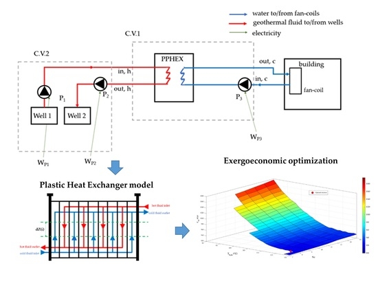
2. Methods and Materials

In this section, the description of PPHEX modeling process is proposed, and the exergoeconomic optimization is introduced. First of all, the mathematical models are defined (see Section 2.1), and then the method used to perform the exergoeconomic analysis is presented (see Section 2.2). Then, the numerical algorithm implemented in the MATLAB environment to obtain the inputs to exergoeconomic analysis, starting from mathematical models’ analysis as described (see Section 2.3). Finally, the methods described in the previous sections have been applied to a case study that is presented in Section 2.4, in which the exergoeconomic analysis introduced in Section 2.2 is detailed for the considered case study.

2.1. Mathematical Models

The mathematical modeling process is distinguished in the geometrical model (see subsection Section 2.1.2), heat exchange model and calculation (see Section 2.1.2), and pressure drops evaluation (see Section 2.1.3). The defined model will return the heat exchange area, plate width, number of plates, and total pressure drops of the PPHEX for a fixed heat power.

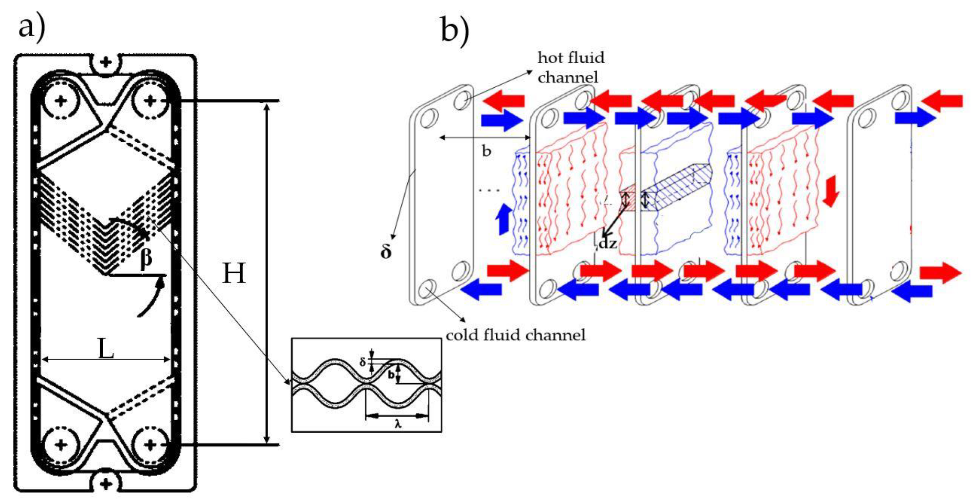
2.1.1. Geometrical Model

The plate heat exchanger consists of a series of plates with corrugated flat flow passages. The hot and cold fluids flow counter-flow in alternate passages are shown Figure 1b. The geometric parameters able to define the plate heat exchanger are shown in Figure 1a,b: plate height (H), plate width (L), chevron angle (β), number of channels for each flow (Nc), wavelength of a sinusoidal surface corrugation or corrugation pitch (𝜆), plate thickness (δ), and plate spacing (b).

In addition, hydraulic diameter (D), corrugation parameter (γ), number of plate (N_p), enlargement factor (φ), and mass flux are defined in

Table 2. Plate heat exchanger parameters.

Parameters	Formulation
hydraulic diameter	$D=2 · b/\phi$
corrugation parameter	$D=\pi · b/\lambda$
number of plates	$N_p=2 · N_c-1$
enlargement factor	$\phi =(1+\sqrt{\left(1+y^2\right)}+4\sqrt{1+\frac{y^2}{2}}$
mass flux	$\mathrm{G}=\dot{m}/\left(\mathrm{L} · \mathrm{Nc} · \mathrm{b}\right)$

, where $\dot{m}$ is the mass flow rate.

2.1.2. Heat Transfer Model and Calculation

The PPHEX model is developed by imposing the desired thermal power (${\dot{Q}}_{PPHEX}$) resulting from the heat transfer between the hot geothermal fluid and the cold water circulated in the building hydronic system. Equation (1) allows the calculation of thermal power ${\dot{Q}}_{PPHEX}$, and the PPHEX height is here discretized in elementary section (i), with infinitesimal height (dZ) as graphed in Figure 2. At the inlet section, which corresponds to i = 0, the geothermal hot fluid enters into heat exchanger, and the cold fluid exits. In this section, the outlet temperature of cold fluid is $T_{out,c}$, and the hot temperature of inlet fluid is $T_{in,c}$ The elementary thermal power in the infinitesimal height dZ ($\delta {\dot{Q}}_{PPHEX,dZ\left(i\right) }$) is calculated according to Equation (2), by considering an adiabatic in which there is no exchange for heat between PPHEX and surroundings. In each elementary section (i), the overall heat transfer coefficient U is evaluated by proper heat transfer correlations, as reported in the following discussion. After the calculation of $\delta {\dot{Q}}_{PPHEX,dZ\left(i\right) }$, the local temperatures associated to the elementary dZ (i + 1) are evaluated by Equations (3) and (4) for geothermal hot fluid and cold fluid, respectively. The temperatures are corrected by also taking into account the pressure drops (see Section 2.1.3).

$${\dot{Q}}_{PPHEX}=\underset{0}{\overset{H}{{\displaystyle \int }}}\left(U·\Delta T·L·\phi \left(2·Nc-1\right)\right) dZ$$

(1)

$$\delta {\dot{Q}}_{PPHEX,dZ\left(i\right) }=dA·U·\left(T_{h,dZ\left(i\right)}-T_{c,dZ\left(i\right)}\right)$$

(2)

$$T_h\left(i+1\right)=T_h\left(i\right)-\frac{\delta {\dot{Q}}_{PPHEX,dZ\left(i\right) }}{{\dot{m}}_h·c_h}$$

(3)

$$T_c\left(i+1\right)=T_c\left(i\right)+\frac{\delta {\dot{Q}}_{PPHEX,dZ\left(i\right) }}{{\dot{m}}_c·c_c}$$

(4)

The overall heat transfer coefficient U is calculated in Equation (5), by considering the convective thermal resistance of hot fluid (${\alpha }_h$) and cold fluid (${\alpha }_c$), the conductive thermal resistance of polymeric material ($k_w$), and fouling resistance for both fluids ($R_{f,c}$, $R_{f,h}$) [27].

$$U=\frac{1}{\frac{1}{{\alpha }_h}+\frac{1}{{\alpha }_c}+\frac{\delta }{k_w}+R_{f,c}+R_{f,h}}.$$

(5)

The heat transfer coefficients are both calculated by Equation (6), where the Nusselt number (N_u) is obtained by Martin equation for liquid fluids, as reported in Equation (7) [28], where k is the fluid conductivity, f is the Fanning friction factor (Equation (8)), and f₀ and f₁ are calculated from Reynolds number.

$$\alpha =Nu·\frac{k}{D}$$

(6)

$$Nu=0.205·P{r}^{\frac{1}{3}}·{\left(\frac{{\mu }_f}{{\mu }_w}\right)}^{1/6}·{\left(f·R{e}^2·sin \left(2\beta \right)\right)}^{0.314}$$

(7)

$$\frac{1}{\sqrt{f}}=\frac{\cos \left(\beta \right)}{{\left(0.045·\tan \left(\beta \right)+0.09·\cos \left(\beta \right)+\frac{f_0}{\cos \left(\beta \right)}\right)}^{0.5}}+\frac{1-\cos \left(\beta \right)}{\sqrt{3.8·f_1}}$$

(8)

2.1.3. Pressure Drops Calculation

The local pressure is evaluated by integration of the pressure drop relations. Then, pressure drops are used to correct the thermodynamic properties in the energy balance (Equations (3) and (4)) by using the REFPROP library. The overall pressure drops, for both fluids, are evaluated by considering three contributions, as expressed in Equation (9) [29]. The first term ($d{p}_{fric})$ considers the loss caused by the friction contribution in the plates, the second term ($d{p}_{mon})$ is the momentum effect, and the last term ($d{p}_{elev})$ considers the elevation change.

$$\frac{dp}{dZ}=\frac{d{p}_{fric}}{dZ}+\frac{d{p}_{mon}}{dZ}+\frac{d{p}_{elev}}{dZ}.$$

(9)

The friction factor term can be determined by using Equation (10) [30], where G is the mass flux, and ${\rho }_m$ is the density average value.

$$d{p}_{fric}=\frac{4·f·dZ·G^2}{2·D·{\rho }_m}.$$

(10)

The momentum pressure drops can be evaluated by using Equation (11), where ${\rho }_{out}$ and ${\rho }_{in}$ represent the density of fluid at outlet and inlet condition of each section area, respectively.

$$d{p}_{mon}=G^2·\left(\frac{1}{{\rho }_{out}}-\frac{1}{{\rho }_{in}}\right).$$

(11)

In this study, this contribution can be neglected because both fluids are in liquid phase during the process. The elevation term (Equation (12)) determines a positive effect on the geothermal fluid that flows downward; on the contrary, it determines a negative effect on the cold water that flows upward. In Equation (12), g is the gravitational acceleration (m·s⁻²).

$$d{p}_{elev}=\pm {\rho }_m·g·dZ.$$

(12)

In addition, the pressure drops due to the inlet manifold is evaluated by considering Equation (13), where $n_p$ is the number of passes in the plate heat exchanger, and $G_{man}$ is the mass flux in the manifold.

$$\Delta p_{man}=\frac{1.5·n_p·G_{man}^2}{2{\rho }_{in}}.$$

(13)

2.2. Exergoeconomic Analysis

The current study proposes the exergoeconomic analysis of a geothermal heating direct system for a single building by assessing the effect of two variables: the number of plates/channels for PPHEX and the inlet temperature of the geothermal fluid. The first one is an endogenous variable whose value is determined through the heat exchanger model. The inlet geothermal fluid temperature is an exogenous variable determined outside the model, and it depends on the specific application (low-medium temperature geothermal fluid). These variables are selected because they substantially influence the results of exergoeconomic analysis. This approach that analyzes the exergoeconomic optimization results referred to an energy system by varying an exogenous and an endogenous variable is widely used in scientific literature [31,32,33].

The exergoeconomic performance of the system has been evaluated for each combination of these parameters. The optimal operating conditions have been selected by means of an exergoeconomic optimization aimed to minimize the exergoeconomic costs associated the thermal energy supplied to the building, which represents the product of the exergoeconomic analysis. All the irreversibility of the process are calculated by using the exergy destruction rate of system(${\dot{I}}_{tot}).$ According to the Gouy–Stodola theorem, it is be evaluated by multiplying the reference or ‘‘dead-state’’ temperature, T₀, by the entropy generation rate, ${\dot{S}}_{gen,tot}$, as reported in Equation (14) [34].

$${\dot{I}}_{tot}=T_0·{\dot{S}}_{gen,tot}$$

(14)

The exergy destruction rate of system can be determined as the difference between the external exergy resources “required” to sustain the total process itself (${\dot{F}}_j$)and the exergy “product” term that constitutes the purpose of the process ($\dot{P}$), as reported in Equation (15).

$${\dot{I}}_{tot}={\displaystyle \sum }_{j=1}^n{\dot{F}}_j-\dot{P}.$$

(15)

Thus, the exergoeconomic cost ($C_{tot}$) to obtain the desired product ($\dot{P}$) analysis is written for yearly exergetic cost (Equation (16)) by including the depreciated investment costs, expressed as the product between the purchased costs $\left(Z_k\right)$ and the Capital Recovery Factor (CRF) for each k-esimo component, and the operating costs, evaluated as a product between the exergetic stream (${\dot{F}}_j$), the related specific exergetic cost ($c_{F,j})$,and the yearly operating hours ($\mathsf{\theta }$). In Equation (16), nc is the total number of components, and the maintenance cost is neglected [31].

$$C_{tot}={\displaystyle \sum }_{j=1}^n{\dot{F}}_j·c_{F,j}·\mathsf{\theta }+\mathrm{CRF}{\displaystyle \sum }_{k=1}^{nc}{Z}_k$$

(16)

CRF is defined as:

$$\mathrm{CRF}=\frac{a{\left(1+a\right)}^m}{{\left(1+a\right)}^m-1}$$

(17)

where a is the interest rate, and m is the service life of the system.

2.3. The Heat Exchanger Modeling and Exergoeconomic Analysis Algorithm

In this section, the numerical algorithm is defined, and the flow chart is represented in Figure 3. It is implemented in MATLAB [35] by means of a main code for exergoeconomic analysis and different functions to evaluate thermodynamic and geometrical properties by using the REFPROP software library [29]. The model returns the heat exchanger surface area ($A_{PPHEX }$) needed to obtain the desired thermal power, ($\delta {\dot{Q}}_{PPHEX,dZ\left(i\right) }$) and the calculation is carried out for each couple of endogenous and exogenous variables (the number of plates/channels for PPHEX and the hot geothermal fluid inlet temperature) in the corresponding range of variation of each variable.

The geometrical input data are width, thickness, plate spacing, chevron angle, wavelength, and others of PPHEX, while the thermodynamic input parameters are the inlet ($T_{c,in }$) and outlet temperature of cold fluid ($T_{c,out }$) and the hot fluid temperature variation ($\Delta T_{h,in-out }$). Moreover, the conductivity of the polymer is imposed as input data.

At that first step of integration that corresponds to i = 1, the fixed parameters are assigned. The pressure drops, and the overall heat transfer coefficient U for both fluids in each dZ are calculated by using Equations (5)–(13). In this way, the elementary heat power $\delta {\dot{Q}}_{PPHEX,dZ\left(i\right) }$ is achieved from Equation (2). By considering the hypothesis of an adiabatic heat exchanger through its surroundings, and by means of the Equations (3) and (4), the temperatures of both fluids in subsequent integration steps (i + 1) are calculated. The integration stops when the desired heat power (${\dot{Q}}_{PPHEX,obj }$) is obtained. The output parameters are geometrical results about heat exchanger surface area ($A_{PPHEX}$) and also the plate height (H), the U, and global pressure drops. As said before, this calculation is conducted by varying $T_{h,in}$ and $N_c$; for this reason, for each output parameter, a matrix ($\stackrel{·}{X}\left(T_{h,in} \times N_c\right)$) is obtained. The first control is made on a limit for pressure drops in the plate, and, according to the PPHEX datasheet, this limit is fixed to 0.5 bar for each fluid flow. The heat exchanger height and area have been directly used in the exergoeconomic cost function, while the pressure drops and the temperature trend have been used as a filter to discard the impossible technical solutions. Once the unacceptable solutions are discarded, the exergoeconomic function is minimized to find the condition with minimum thermoeconomic impact for single building.

2.4. The Case Study

The methods described in the previous sections have been applied to a case study in Italy. More precisely, the Phlegrean Fields area (south of Italy) has been chosen for this application. It is an active volcano district of the Campania region characterized by high geothermal fluid temperature at shallow depth [26,36,37]. In particular, as it is possible to derive from previous analyses conducted in this area, a temperature of geothermal fluid in the range 90–120 °C has already been recorded at the depth of 86–101 m. Thus, the results of the exergoeconomic optimization are referred to this specific area, and they will be different if the same methodology is applied to a different zone with a potential interest from geothermal point of view (low-medium temperature geothermal fluid availability).

Thus, this case study takes into account the possibility to use a geothermal PPHEX of 24 kW_th connected to the hydronic building heating system by means of a thermal grid. As reported in the Figure 4, the geothermal fluid is drawn from the ground by using the production well (1) and the first pump (P₁), and, after, it enters in the control volume C.V.1. In C.V.1., the geothermal fluid heats the cold water, and, after, it is reinjected by using P₂ and injection well (2). The hot water exiting the PPHEX is sent to building circuit by means of a circulating pump P₃. The fixed PPHEX parameters are reported in

Table 3. Input Data.

Parameters	Symbol	Value
Inlet Temperature of geothermal hot fluid (°C)	${\mathrm{T}}_{h,in}$	90–120
Temperature difference of geothermal fluid (°C)	$\Delta {\mathrm{T}}_{h,in-out}$	20
Inlet Temperature of cold water (°C)	${\mathrm{T}}_{c,in}$	45
Outlet Temperature of cold water (°C)	${\mathrm{T}}_{c,out}$	60
Thermal polymer conductivity (Wm−1 K−1)	$k_w$	0.22
Plate spacing (mm)	b	2.2
Wavelength of a sinusoidal surface corrugation (mm)	$\lambda$	2
Plate thickness (mm)	δ	0.4
Channels number for each flow (-)	Nc	4–14
Chevron angle	β	60°
Plate width (m)	L	0.077

, according with datasheets [6,7,38]. The variable parameters are the inlet geothermal temperature and the number of channels for each flow (or plates).

The geothermal fluid is extracted from a shallow production well, indeed, according to data about geothermal fields of Phlegrean Fields area (South of Italy) [12,36,37], geothermal fluids in the temperature range of 90–120 °C at a depth varying from 86 m to 101 m. To perform the exergoeconomic analysis in the considered case study, Equations (16) and (17) have been detailed with reference to Figure 4. Referring to C.V.1, the exergy balance can be written as reported in Equation (18), where the term (${\dot{m}}_c·(e{x}_{c,out}-e{x}_{c,in}$)) represents the exergy product ($\dot{P}$) according to Equation (16). The exergy input ($\dot{F}$) is the sum of exergy rate of geothermal fluid (${\dot{m}}_h·(e{x}_{h,in}-e{x}_{h,out}$)) and exergy electric input (${\dot{W}}_{P3}$). The first term can be evaluated by exergy balance on C.V.2 reported in Equation (19), where the exergy input is equal to exergy electric input (${\dot{W}}_{P1}+{\dot{W}}_{P2}$). Thus, the total exergy balance can be expressed according to Equation (20).

$${\dot{m}}_h·e{x}_{h,in}+{\dot{m}}_c·e{x}_{c,in}+{\dot{W}}_{P3}={\dot{m}}_h·e{x}_{h,out}+{\dot{m}}_c·e{x}_{c,out}+{\dot{I}}_{V.C.1}$$

(18)

$${\dot{m}}_h·e{x}_{h,out}+{\dot{W}}_{P1}+{\dot{W}}_{P2}={\dot{m}}_h·e{x}_{h,in}+{\dot{I}}_{V.C.1}$$

(19)

$${\dot{m}}_c·\left(e{x}_{c,out}-e{x}_{c,in}\right)={\dot{W}}_{P3}+{\dot{W}}_{P1}+{\dot{W}}_{P2}-{\dot{I}}_{tot}$$

(20)

Once the exergy balance is defined, the exergoeconomic balance can be defined by using the exergoeconomic cost and the additional purchase costs (according to Equation (16)), as reported in the Equation (21).

$$C_{tot}=c_{F,el}·\mathsf{\theta }·\left({\dot{W}}_{P3}+{\dot{W}}_{P1}+{\dot{W}}_{P2}\right)+CRF·\left(Z_{P1}+Z_{P2}+Z_{P3}+Z_{well,1}+Z_{well,2}+Z_{PHEX}\right)$$

(21)

where $C_{tot}$ is the exergoeconomic cost associated to the product $\dot{P}$, ${\mathrm{c}}_{\mathrm{F},\mathrm{el}}$ is the specific exergoeconomic cost of electric exergy input, $Z_{P1}, Z_{P2}, Z_{P3}$ are the investment costs of pumps, $Z_{well,1},Z_{well,2}$ are the wells costs, and ${\mathrm{Z}}_{\mathrm{PPHEX}}$ is the PPHEX cost. In

Table 4. Cost function.

Component	Investment Cost (€)	Reference
Pump	${\mathrm{Z}}_{\mathrm{P}}=107.26·{\dot{W}}_P^{0.7176}$	[39]
Well	${\mathrm{Z}}_{\mathrm{well}}=23.578·{\mathrm{e}}^{0.0063·{\mathrm{d}}_{\mathrm{well}}}·{\mathrm{H}}_{\mathrm{well}}$	[40]
PPHEX	${\mathrm{Z}}_{\mathrm{PPHEX}}={\mathrm{c}}_{\mathrm{PPHEX}}·A_{\mathit{PPHEX}}$	[6]

, the investment cost functions are listed, where ${\mathrm{H}}_{\mathrm{well}}$ is the deep length of well ranging from 86 to 101 m in Phlegrean Fields area, ${\mathrm{d}}_{\mathrm{well}}$ is the well diameter, and ${\mathrm{c}}_{\mathrm{PPHEX}}$ and A_PPHEX are the specific cost and heat exchange surface area of PPHEX, respectively.

The $Z_{PPHEX}$ is obtained by market investigation, and it results in approximatively equal to 1230 €·m⁻². However, $\mathsf{\theta }$ is equal to 1088 h/y, by taking into account the typical Mediterranean hot climate referred to in the South of Italy. The $c_{el }$ is fixed equal to 0.25 c€·kWh_el⁻¹ VAT included [41].

3. Results and Discussion

In this section, the results of analysis are presented. In Section 3.1, the main outcomes of the mathematical modeling of heat exchanger are discussed. In Section 3.2, the results of exergoeconomic analysis are presented by including the sensitivity analysis about thermodynamic and geometrical parameters.

3.1. Geometrical and Thermodynamic Results

The geometrical characteristics of PPHEX highly affect the pressure drops results. The cold fluid presents higher pressure drops due to greater mass flow rate (0.382 kg·s⁻¹) than hot one (0.287 kg·s⁻¹). The mass flow rate is calculated by energy balance on PPHEX, according to Equations (3) and (4). The best configuration in terms of pressure drops is verified when the geothermal fluid inlet temperature is equal to 90 °C, and the number of channels for each fluid flow is equal to 4. The results obtained by mathematical model are filtered by assuming a maximum acceptable value for ∆p equal to 0.5 bar. In Figure 5, the pressure drops of hot and cold fluid are reported by varying $T_{h,in}$ and Nc. If the inlet temperature of geothermal fluid is equal to its maximum (120 °C), the lowest acceptable Nc is 5 for hot fluid, and 7 for cold fluid. Even if $T_{h,in}$ is equal to its lowest value (90 °C), the acceptable Nc increases up to 6 for hot fluid, and 9 for cold fluid. Thus, pressure drops of the cold fluid ($\Delta p_c$) represent the discriminating factor to filter the results since $\Delta p_c$ is the highest one. Thus, the lowest acceptable Nc is equal to 7.

Following the methodology defined in Equations (3) and (4), the trends of temperatures in the PPHEX are represented for hot and cold fluid in 3D, in Figure 6 and Figure 7, respectively, in the case in which the number of channels are equal to 12, and the $T_{h,in }$ is equal to 115 °C. As a matter of fact, the heat transfer process determines the heating of cold water supplied to the building by the cooling of geothermal fluid. However, the legislation concerning the geothermal uses recommends a reinjection temperature of geothermal fluid not lower than 70 °C [42]. Thus, in order to ensure the recommended reinjection temperature, the minimum considered geothermal fluid inlet temperature is 95 °C. Figure 6 and Figure 7 also show the flows direction. More precisely, in Figure 6, the geothermal hot fluid enters from the PPHEX in the upper side, and its temperature decreases to 20 °C, as far as the exit section (H = 0 mm). In Figure 7, the cold fluid enters from the PPHEX down side, and its temperature increases from 45 to 60 °C (15 °C) as far as the exit section that corresponds to geothermal fluid entry. The temperature difference of both fluids along the height of the heat exchanger is the same because they are assimilated to liquid water in the model by using the REFPROP library. This fact is justified by the same color trend of both 3D Figure 6 and Figure 7, even if the temperature variation range represented by the colors bars is significantly different (115–95 °C for hot fluid (Figure 6) and 60–45 °C for cooling fluid (Figure 7)).

According to the methodology defined in the Equations (5)–(7), the calculation of overall heat transfer coefficient (U) has been obtained for each combination of the two variables ($T_{h,in }$ and Nc) filtered by considering the restrictions on pressure drops (0.5 bar). In Figure 8, the surface plot of U is showed. The blue bar represents the condition with the lowest U value (225–230 W·m⁻²·K⁻¹) that is verified when Nc is higher than 9. U presents the greatest value (248 W·m⁻²·K⁻¹) when Nc is equal to 7, and $T_{h,in }$ is equal to 118–120 °C. The $T_{h,in }$ slightly influences the overall heat transfer coefficient: for a fixed value of Nc, and by varying $T_{h,in }$ from 120 to 90 °C, the U value shows an increase lower than 1%. Differently, by fixing the temperature, and by considering a number of channels variation from 4 to 14, the U value increases up to 10%. This can be explained by taking into account the fact that the heat transfer convective coefficient (α) is strongly influenced by mass flux (G), which assumes higher values when Nc decreases due to the reduction of the crossing flow section. However, the variation range of U is very low (225–248 W·m⁻²·K⁻¹) because both fluids are in liquid phase, and the plate heat exchanger presents low room for improvement.

For filtered solutions, the heat exchange surface area of PPEHX is reported in

Table 5. Heat exchange surface area for matching Nc-$T_{h,in}$ solution.

Polymer Plate Heat Exchange Surface Area APPHEX (m2)
T (°C)	Nc 7	8	9	10	11	12	13	14
90	-	-	-	3.73	3.78	3.83	3.87	3.91
91	-	-	-	3.60	3.66	3.69	3.74	3.78
92	-	-	-	3.47	3.53	3.58	3.62	3.65
93	-	-	3.31	3.36	3.41	3.45	3.50	3.52
94	-	-	3.21	3.25	3.31	3.33	3.38	3.41
95	-	-	3.11	3.16	3.21	3.24	3.28	3.31
96	-	-	3.01	3.07	3.10	3.15	3.19	3.20
97	-	-	2.93	2.98	3.02	3.04	3.09	3.13
98	-	-	2.84	2.88	2.92	2.98	2.99	3.05
99	-	-	2.76	2.81	2.84	2.89	2.92	2.94
100	-	-	2.70	2.74	2.78	2.80	2.85	2.86
101	-	-	2.63	2.66	2.70	2.73	2.77	2.78
102	-	2.51	2.55	2.59	2.63	2.66	2.70	2.73
103	-	2.45	2.50	2.53	2.57	2.60	2.63	2.65
104	-	2.39	2.43	2.48	2.51	2.53	2.58	2.60
105	-	2.33	2.38	2.40	2.45	2.48	2.50	2.52
106	-	2.28	2.31	2.35	2.39	2.42	2.46	2.47
107	-	2.23	2.27	2.31	2.33	2.37	2.38	2.42
108	-	2.17	2.22	2.25	2.29	2.30	2.33	2.36
109	-	2.13	2.17	2.20	2.23	2.26	2.29	2.31
110	-	2.09	2.12	2.16	2.19	2.21	2.24	2.26
111	-	2.04	2.08	2.11	2.14	2.17	2.19	2.23
112	-	2.00	2.03	2.07	2.10	2.13	2.14	2.18
113	-	1.96	2.00	2.03	2.06	2.08	2.12	2.13
114	-	1.93	1.95	2.00	2.02	2.04	2.07	2.10
115	-	1.88	1.92	1.96	1.98	2.01	2.02	2.05
116	-	1.85	1.89	1.92	1.94	1.97	1.99	2.02
117	-	1.81	1.85	1.89	1.90	1.92	1.95	1.97
118	1.74	1.78	1.82	1.85	1.88	1.90	1.92	1.94
119	1.72	1.75	1.79	1.81	1.84	1.86	1.87	1.92
120	1.68	1.72	1.75	1.77	1.80	1.83	1.85	1.86

. It presents a highest value equal to 3.91 m² when Nc = 14, and $T_{h,in }$ = 90 °C, while the lowest value is equal to 1.68 m² when Nc = 7, and $T_{h,in }$ = 120 °C. The maximum percentage variation of $A_{PPHEX}$ is equal to 57%. So, the optimum solution, in terms of lower footprint, corresponds with best heat transfer performance.

3.2. Exergoeconomic Results

As mentioned above, the optimization of the two investigated parameters, the temperature of the geothermal source and number of channels, is carried out in order to find the configuration that guarantees the lower exergoeconomic cost of product, $C_{tot}$. First of all, the investment cost of PPHEX is represented in Figure 9. The configuration that leads to the lowest investment cost corresponds to the condition with the smallest heat exchange surface area (Nc = 7 and $T_{h,in }$ = 120 °C), in which $Z_{PPHEX}$ amounts to 2069 €. The investment cost increase occurs when the temperature availability of geothermal fluid decreases, while it is not very influenced by Nc variation. In fact, the increasing temperature of 1 K of geothermal fluid corresponds to an investment cost average rise of 2.5% when Nc is fixed to 14. However, by considering temperatures lower than 100 °C, the investment cost is higher than 3000 €. Moreover, if the Nc is decreases up to 10, the investment cost drops below 2000 €, when the geothermal fluid temperatures are to 120 °C.

The variation of the main exergoeconomic costs as function of Nc and $T_{h,in }$ is illustrated in Figure 10. The exergoeconomic cost of electricity, $C_{el },$ calculated in first term of Equation (21), is caused by electricity consumption of pumps during heating period. It dramatically increases as the geothermal fluid temperature grows because the pressure drops, and the deep well rises, while it presents a low variation with Nc, as depicted in Figure 10a. For Nc fixed to its maximum value (14), the yearly exergetic cost of electricity is equal to 213 €·y⁻¹ if $T_{h,in }$ is 90 °C, and 245 €/y if $T_{h,in }$ amounts to 120 °C, presenting a percentage variation of 13%. By fixing $T_{h,in }$ to 120 °C, the electricity exergoeconomic cost is equal to 255 €·y⁻¹ if Nc decreases to 7, showing a percentage variation of 4%. Figure 10b illustrates the yearly amortized cost of PPHEX. It reaches the highest values when the geothermal fluid temperature is lower than 96 °C; thus, in this condition, the exergoeconomic PPHEX cost is greater than 350 €·y⁻¹. Nc determines a not very relevant influence on the cost of PPHEX, too. Indeed, in each temperature condition, the exergoeconomic cost increases of 10% for Nc ranging from 7 to 14. The lowest values (≤250 €/y) can be obtained when $T_{h,in }$ varies from 110 to 120 °C. Figure 10c shows the amortized cost of three pumps of system. According to electricity cost, the pumps investment costs need higher power capacity if the temperature increases determining higher purchase costs. Despite this, a higher influence in pumps investment cost is determined by Nc variation. Overall, this cost slightly influences the system because its maximum is 12.6 €·y⁻¹, and its minimum is 10.8 €·y⁻¹. Figure 10d shows the most expensive exergoeconomic parameter of geothermal plant: the well cost. As expected, this cost increases with depth and temperature increase, and it is not influenced by heat exchanger geometry. The highest value corresponds to 455 €·y⁻¹, and the lowest one is 390 €·y⁻¹.

In Figure 11, the optimization of global exergoeconomic analysis is represented. The convenience of investment is presented by blue and light-blue solution that correspond to temperature of geothermal fluid higher than 105 °C. In these conditions, for each number of channels, $C_{tot }$ is lower than 950 €·y⁻¹. Both $T_{h,in }$ and Nc affect the total exergoeconomic costs of the product, but, for a fixed temperature, and for a changing of Nc from 7 to 14, the variation of $C_{tot }$ is equal to 1.6%. However, by varying $T_{h,in }$ from 90 to 120 °C for a fixed Nc, the variation of $C_{tot }$ corresponds to 13%. Despite the well cost and electricity cost increase with temperature rise, the product exergoeconomic cost presents an opposite behavior with temperature. The product yearly cost is highly influenced by the exergoeconomic investment cost of PPHEX. This result is due the fact that, even if the drilling costs are usually the large portion of costs in a geothermal plant, in Phlegrean Fields, the increase of well depth to go from a geothermal fluid temperature of 90 °C to 120 °C is equal to only 15 m (from 86 m to 101 m in depth). Thus, these outcomes are strongly related to the area in which the exergoeconomic analysis is conducted. When the number of channels for each flow is equal to 10, and the temperature increases from 90 to 120 °C, the percentage variations of exergoeconomic yearly cost are equal to 13.8%, 16.8%, and −52.5% for electricity pumping, well, and PPHEX investment, respectively. Finally, the product exergoeconomic cost shows a decrease of 12.8%, varying $T_{h,in }$ from 90 to 120 °C. The optimum solution equal to 922 €·y⁻¹ is found for Nc equal to 8 that corresponds to 15 plates, and 117 °C of geothermal hot inlet temperature.

4. Conclusions

This research paper presented a model and analysis of a heating system for single building operating in geothermal field from the thermodynamic and thermoeconomic viewpoints. An advanced mathematical model was used to design a plastic heat exchanger to overcome the fouling problems that affect the heat exchangers of a geothermal plant. The results of model were used as input for an exergoeconomic optimization to evaluate the thermoeconomic performance of system by varying thermodynamic and geometric parameters. Then, the general methodology was applied to a case study in which the modeled polymeric plate heat exchanger interacting with the geothermal fluid was used, to meet the space heating need of a single building located in the active volcano district of the Campania region. The results are summarized in the following:

• the overall heat exchanger coefficient presents the greatest values for high temperature of geothermal fluid (105–120 °C) and for a number of channels for each flow variable from 7 to 12;
• the required heat exchanger surface areas are low (and, consequently, the HEX purchase cost) for overall heat exchanger coefficient equal about to 240–250 W/K·m²;
• the investment cost of heat exchanger decreases when the inlet geothermal temperature increases; on the contrary, the well investment and the electricity cost increases with temperature;
• the variation of well and electricity exergoeconomic costs is lower than heat exchanger one; thus, the product exergoeconomic cost shows a trend similar to heat exchanger cost; and
• the minimum value for product is equal to 922 €·y⁻¹, and it occurs when the geothermal hot inlet temperature is equal to 117 °C, and Nc is equal to 8, that corresponds to 15 plates.

As a general conclusion, the development of this research allows the thermodynamic improvements and potential cost reductions in a geothermal plant for direct air conditioning applications. In future works, the investigation of multi-users system will be defined by using higher variable parameters in the exergoeconomic analysis, and the validation of these results could be conducted in the framework of GEOGRID project.

References

1. New Rules for Greener and Smarter Buildings Will Increase Quality of Life for All Europeans. Available online: https://ec.europa.eu/info/news/new-rules-greener-and-smarter-buildings-will-increase-quality-life-all-europeans-2019-apr-15_en (accessed on 19 July 2021).
2. Eurostat. Distribution of Population by Degree of Urbanisation, Dwelling Type and Income Group. 2020. Available online: https://appsso.eurostat.ec.europa.eu/nui/show.do?dataset=ilc_lvho01&lang=en (accessed on 19 July 2021).
3. International Energy Agency. Data and Statistics. 2021. Available online: https://www.iea.org/data-and-statistics/data-browser?country=WORLD&fuel=Electricity%20and%20heat&indicator=HeatGenByFuel (accessed on 19 July 2021).
4. Lund, J.W.; Toth, A.N. Direct utilization of geothermal energy 2020 worldwide review. Geothermics 2021, 90, 101915. [Google Scholar] [CrossRef]
5. Tan, M.; Karabacak, R.; Acar, M. Experimental assessment the liquid/solid fluidized bed heat exchanger of thermal performance: An application. Geothermics 2016, 62, 70–78. [Google Scholar] [CrossRef]
6. CALORPLAST. Shell and Tube Heat Exchanger. Data Sheet. Available online: https://www.calorplast-waermetechnik.de/wp-content/uploads/liquid-liquid-heat-exchanger.pdf (accessed on 12 October 2021).
7. TMW Technologies. Plastic Plate Heat Exchanger. Data Sheet. Available online: https://pdf.directindustry.com/pdf/tmw-technologies/plastic-heat-exchanger/168190-760122.html (accessed on 12 October 2021).
8. ELRINGKLINGER. Shell and Tube Heat Exchanger. Data Sheet. Available online: https://www.elringklinger-engineered-plastics.com/fileadmin/user_upload/ekkt/downloads/kataloge/englisch/thermo-x_heat_exchanger.pdf (accessed on 12 October 2021).
9. HeatMatrix Group. Polymer Economiser. Data Sheet. Available online: https://heatmatrixgroup.com/products/economiser/ (accessed on 12 October 2021).
10. Chen, X.; Su, Y.; Reay, D.; Riffat, S. Recent research developments in polymer heat exchangers—A review. Renew. Sustain. Energy Rev. 2016, 16, 1367–1386. [Google Scholar]
11. T’Joen, C.; Park, Y.; Wang, Q.; Sommers, A.; Han, X.; Jacobi, A. A review on polymer heat exchangers for HVAC&R applications. Int. J. Refrig. 2009, 32, 763–779. [Google Scholar]
12. Ceglia, F.; Macaluso, A.; Marrasso, E.; Sasso, M.; Vanoli, L. Modelling of polymeric shell and tube heat exchangers for low-medium temperature geothermal applications. Energies 2020, 13, 2737. [Google Scholar] [CrossRef]
13. Ceglia, F.; Marrasso, E.; Roselli, C.; Sasso, M. Effect of layout and working fluid on heat transfer of polymeric shell and tube heat exchangers for small size geothermal ORC via 1-D numerical analysis. Geothermics 2021, 95, 102118. [Google Scholar] [CrossRef]
14. Luo, X.; Wang, Y.; Zhao, J.; Chen, Y.; Mo, S.; Gong, Y. Grey relational analysis of an integrated cascade utilization system of geothermal water. Int. J. Green Energy 2016, 13, 14–27. [Google Scholar] [CrossRef]
15. Arslan, O.; Kose, R. Exergoeconomic optimization of integrated geothermal system in Simav, Kutahya. Energy Convers. Manag. 2010, 51, 663–676. [Google Scholar] [CrossRef]
16. Jamil, M.A.; Goraya, T.S.; Shahzad, M.W.; Zubair, S.M. Exergoeconomic optimization of a shell-and-tube heat exchanger. Energy Convers. Manag. 2020, 226, 113462. [Google Scholar] [CrossRef]
17. Hajabdollahi, H.; Naderi, M.; Adimi, S. A comparative study on the shell and tube and gasket-plate heat exchangers: The economic viewpoint. Appl. Therm. Eng. 2016, 92, 271–282. [Google Scholar] [CrossRef]
18. Ozgener, L.; Hepbasli, A.; Dincer, I. Thermodynamic analysis of a geothermal district heating system. Int. J. Exergy 2005, 2, 231–245. [Google Scholar] [CrossRef]
19. Hajabdollahi, H.; Ahmadi, P.; Dincer, I. Thermoeconomic optimization of a shell and tube condenser using evolutionary algorithm. Int. J. Refriger. 2011, 34, 1066–1076. [Google Scholar] [CrossRef]
20. Hajabdollahi, H. Investigating the effect of non-similar fins in thermoeconomic optimization of plate fin heat exchanger. Appl. Therm. Eng. 2015, 82, 152–161. [Google Scholar] [CrossRef]
21. Hajabdollahi, H.; Tahani, M.; Fard, M.H.S. CFD modeling and multi-objective optimization of compact heat exchanger using CAN method. Appl. Therm. Eng. 2011, 31, 2597–2604. [Google Scholar] [CrossRef]
22. Gemitzi, A.; Dalampakis, P.; Falalakis, G. Detecting geothermal anomalies using Landsat 8 thermal infrared remotely sensed data. Int. J. Appl. Earth Obs. Geoinf. 2021, 96, 102283. [Google Scholar] [CrossRef]
23. Lund, J.W.; Toth, A.N. Direct utilization of geothermal energy 2020 worldwide review. In Proceedings of the World Geothermal Congress 2020+1, Reykjavik, Iceland, 27 April 2021; Available online: https://www.geothermal-energy.org/pdf/IGAstandard/WGC/2020/01018.pdf (accessed on 21 October 2021).
24. Hurter, S.; Schellschmidt, R. Atlas of geothermal resources in Europe. Geothermics 2003, 32, 779–787. [Google Scholar] [CrossRef]
25. Ates, H.K.; Serpen, U. Power plant selection for medium to high enthalpy geothermal resources of Turkey. Energy 2016, 102, 287–301. [Google Scholar] [CrossRef]
26. Carlino, S.; Troiano, A.; Di Giuseppe, M.G.; Tramelli, A.; Troise, C.; Somma, R.; De Natale, G. Exploitation of geothermal energy in active volcanic areas: A numerical modelling applied to high temperature Mofete geothermal field, at Campi Flegrei caldera (Southern Italy). Renew. Energy 2016, 84, 54–66. [Google Scholar] [CrossRef]
27. Çengel, Y.A. Thermodynamics and Heat Transfer; McGraw-Hill: New York, NY, USA, 2008; ISBN 0-390-86122-7. [Google Scholar]
28. Shah, R.K.; Seculić, D.P. Foundamental of Heat Exchanger Design. John Wiley & Sons, Inc.: Hoboken, NJ, USA, 2003. [Google Scholar]
29. Lemmon, E.W.; Huber, M.L.; McLinden, M.O. Reference Fluid Thermodynamic and Transport Properties, Nist Standard Reference Database 23; Version 9.1; Physical and Chemical Properties Division, NIST: Boulder, CO, USA, 2002.
30. Martin, H. A theoretical approach to predict the performance of chevron-type plate heat exchangers. Chem. Eng. Process. Process. Intensif. 1996, 35, 301–310. [Google Scholar] [CrossRef]
31. D’Accadia, M.D.; Fichera, A.; Sasso, M.; Vidiri, M. Determining the optimal configuration of a heat exchanger (with a two-phase refrigerant) using exergoeconomics. Appl. Energy 2002, 71, 191–203. [Google Scholar] [CrossRef]
32. Di Fraia, S.; Macaluso, A.; Massarotti, N.; Vanoli, L. Geothermal energy for wastewater and sludge treatment: An exergoeconomic analysis. Energy Convers. Manag. 2020, 224, 113180. [Google Scholar] [CrossRef]
33. D’Accadia, M.D.; Sasso, M. Exergetic cost and exergoeconomic evaluation of vapour-compression heat pumps. Energy 1998, 23, 937–942. [Google Scholar] [CrossRef]
34. Kotas, T.J. The Exergy Method of Thermal Plant Analysis; Butterwoths: London UK, 1995. [Google Scholar]
35. MATLAB and Statistics Toolbox Release; The MathWorks, Inc.: Natick, MA, USA, 2018.
36. Carlino, S.; Somma, R.; Troiano, A.; DI Giuseppe, M.G.; Troise, C.; DE Natale, G. The geothermal system of Ischia Island (southern Italy): Critical review and sustainability analysis of geothermal resource for electricity generation. Renew. Energy 2014, 62, 177–196. [Google Scholar] [CrossRef]
37. Carlino, S.; Somma, R.; Troise, C.; DE Natale, G. The geothermal exploration of Campanian volcanoes: Historical review and future development. Renew. Sustain. Energy Rev. 2012, 16, 1004–1030. [Google Scholar] [CrossRef]
38. Weinmann, S. Available online: https://www.weinmann-schanz.de/gb/en/Heating/Solar-technology-geothermal-energy/Plate-heat-exchangers-and-accessories/Plate-heat-exchanger-ZB/Plate-heat-exchanger-P20-4x-3-4-ET-20-KW-20-plates-ZB-10-20-sid515394.html (accessed on 19 July 2021).
39. Casasso, A.; Sethi, R.; Rivoire, M. Studio di Fattibilità Per un Impianto Geotermico a Circuito Aperto in un Complesso Residenziale (Feasibility Study For an Open Circuit Geothermal Plant in a Residential Context). Master’s Thesis, Politecnico di Torino, Torino, Italy, 2018. [Google Scholar]
40. Catalogue of Operational Criteria and Constraints for Shallow Geothermal Systems in the Alpine Environment. Available online: https://www.alpine-space.eu/projects/greta/deliverables/d3.2.1_catalogue-of-operational-criteria-and-constraints--update2a--2018.pdf (accessed on 5 August 2021).
41. ARERA. Italian Document: Andamento del Prezzo dell’Energia Elettrica per il Consumatore Domestico Tipo in Maggior Tutela. Data of First Semester 2021. 2021. Available online: https://www.arera.it/it/dati/eep35.htm (accessed on 15 March 2021).
42. Franco, A.; Villani, M. Optimal design of binary cycle power plants for water-dominated, medium-temperature geothermal fields. Geothermics 2009, 38, 379–391. [Google Scholar] [CrossRef] [Green Version]
Figure 1. Geometry (a) and heat transfer process (b) of the plate heat exchanger.
Energies 14 06994 g001
Figure 2. Plate heat exchanger height discretization.
Energies 14 06994 g002
Figure 3. Algorithm flow chart.
Energies 14 06994 g003
Figure 4. Geothermal heating direct process.
Energies 14 06994 g004
Figure 5. Pressure drops in cold (a) and hot fluid (b).
Energies 14 06994 g005
Figure 6. Temperature trend of hot geothermal fluid for Nc = 12 and T h , i n = 115 °C.
Energies 14 06994 g006
Figure 7. Temperature trend of cold water for Nc = 12 and T h , i n = 115 °C.
Energies 14 06994 g007
Figure 8. Overall heat transfer coefficient.
Energies 14 06994 g008
Figure 9. Heat exchanger investment cost.
Energies 14 06994 g009
Figure 10. Effect of Nc and T h , i n on the exergoeconomic costs of electricity (a), on PPHEX purchase cost (b), on pumps purchase cost (c), and on well investment cost (d).
Energies 14 06994 g010
Figure 11. Total exergoeconomic cost minimization.
Energies 14 06994 g011