Research on Optimal Torque Control of Turning Energy Consumption for EVs with Motorized Wheels

Abstract

This paper aims to explore torque optimization control issue in the turning of EV (Electric Vehicles) with motorized wheels for reducing energy consumption in this process. A three-degree-of-freedom (3-DOF) vehicle dynamics model is used to analyze the total longitudinal force of the vehicle and explain the influence of torque vectoring distribution (TVD) on turning resistance. The Genetic Algorithm-Particle Swarm Optimization Hybrid Algorithm (GA-PSO) is used to optimize the torque distribution coefficient offline. Then, a torque optimization control strategy for obtaining minimum turning energy consumption online and a torque distribution coefficient (TDC) table in different cornering conditions are proposed, with the consideration of vehicle stability and possible maximum energy-saving contribution. Furthermore, given the operation points of the in-wheel motors, a more accurate TDC table is developed, which includes motor efficiency in the optimization process. Various simulation results showed that the proposed torque optimization control strategy can reduce the energy consumption in cornering by about 4% for constant motor efficiency ideally and 19% when considering the motor efficiency changes in reality.

1. Introduction

The energy crisis and environmental pollution are important issues for all countries in the world currently, while the automobile industry is one of the iconic industries of social development and technological progress. Reducing environmental contamination and energy consumption has become the concern for industry professionals. Therefore, it has become a consensus all over the world that the development of new energy vehicles, especially electric vehicles, must be accelerated.

The unique advantages of four-wheel independent-drive (4WID) technology in flexible torque control, improving vehicle stability and smoothness, etc., contribute to its more extensive application in electric vehicles. Comparatively, the FWID has the weakness of generality in practical application, which places more attention on improving the handling and stability of the vehicle. Additionally, TVD technology applied in 4WID-EVs can greatly reduce the energy consumption of the entire vehicle in corners, thus improving energy conservation [1,2]. At present, for TVD technology, many scholars and experts have proposed relevant algorithms and fusion technologies to improve vehicle-handling stability and energy efficiency [3,4], as well as the vehicle dynamics performance [5].

Koehler proposed the use of the LQR algorithm to calculate the required yaw moment of the vehicle and combined the characteristics of motor efficiency to distribute torque to each wheel so as to realize the function of TVD [6]. Wang raised a differential drive assisted steering (DDAS) system that uses an electric wheel drive system to differentially distribute the torque of the left and right front wheels to reduce the energy consumption of the steering system [7]. Alipour used the fuzzy controller to obtain the reference longitudinal speed and target the yaw rate of the vehicle in TVD control [8]. Wang et al. [9] presented a TVD control strategy based on recursive least squares (RLS) identification of tire longitudinal stiffness, which effectively reduced the average slip rate of the drive shaft and improved the cornering efficiency. Yu et al. [10] designed a 4WD-EVs steering stability hierarchical control strategy, which combined sliding-mode yaw stability control with rolling time-domain torque-coordinated and optimized distribution control to improve the steering stability and driving safety. Sun et al. [11] improved the torque vector on the rear wheels of ID-EVs to increase the driving efficiency of the vehicle by 4% under typical operating conditions. Wong proposed a Holistic Corner Controller (HHC) suitable for 4WID-EVs, using motor MAP directly, according to the instantaneous operating point of the motor, which improved the driving efficiency of the vehicle in various working conditions effectively [12].

The calculation and analysis of energy consumption affect the energy flow of cornering vehicles [13,14]. It also led to more accuracy regarding the energy expenditure estimation and energy consumption prediction of EVs [15,16] and then improved the energy management strategy [17].

This paper uses dynamic model creatively to analyze the mechanism of turning resistance theoretically. From this, the influence of TVD on turning resistance and energy consumption is explained clearly. In addition, this article reasonably applies the GA-PSO to obtain the torque optimization control strategy for the minimum turning energy consumption. Considering the actual operating conditions of the vehicle, the optimal torque distribution (OTD) coefficient based on motor working points is obtained through simulation analysis, greatly reducing vehicle energy consumption in corners. Through the hardware-in-the-loop test, the accuracy of the control strategy proposed in this paper is verified.

2. Establishment of a Dynamic Model and Analysis of Longitudinal Force

The yaw rate is the most direct parameter to reflect the cornering characteristics of vehicles. TVD technology can be used to decouple the longitudinal forces of each wheel from each other and generate the yaw moment so that the yaw rate is increased or decreased effectively according to the needs of the actual working conditions. Therefore, it is able to reduce the resistance of the vehicle in corners and reduce the energy consumption. Consequently, the analysis of the longitudinal force of the vehicle is an important foundation for explaining the influence of TVD technology on the turning resistance in principle.

2.1. Establishment of 3-DOF Vehicle Dynamic Model

The vehicle model is simplified to a 3-DOF single-track vehicle model with two tires [18], which can be used to analyze the vehicle turning stability clearly [19,20]. When its radius of curvature is R, and it turns around point P, the stress distribution is shown in Figure 1.

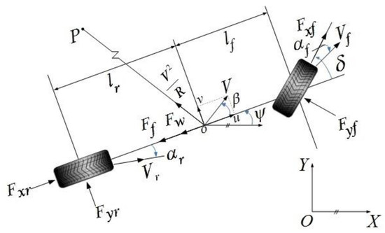
Figure 1. 3-DOF single-track model.

According to Figure 1, three dynamic differential equations of the body moving along the X- and Y-axis and rotating around the Z-axis can be established.

$$m\dot{V}\cos \beta -mV(\dot{\beta }+\dot{\psi })\sin \beta = F_{xf}\cos \delta -F_{yf}\sin \delta +F_{xr}-(F_f+F_w)$$

(1)

$$m\dot{V}\sin \beta +mV(\dot{\beta }+\dot{\psi })\cos \beta = F_{xf}\sin \delta +F_{yf}\cos \delta +F_{yr}$$

(2)

$$J\ddot{\psi } = (F_{xf}\sin \delta +F_{yf}\cos \delta )l_f-F_{yr}{l}_r$$

(3)

where $m$ is the mass of the vehicle; $J$ is the rotational inertia of the vehicle around the vertical axis; $\beta$ is the sideslip angle at the center of gravity (CoG); $\psi$ is the heading angle; $\delta$ is the steering angle of front wheels (FWSA); $l_f$ and $l_r$ are the lengths from the CoG to the front and rear wheel axles, respectively; $F_{xf}$ and $F_{xr}$ are the combined longitudinal tire forces of the front and rear axles, respectively; $F_{yf}$ and $F_{yr}$ are the combined lateral tire forces of the front and rear axles, respectively; $F_f$ is the rolling resistance of the entirety of all wheels; and $F_w$ is the aerodynamic drag on the vehicle body.

Assuming that the current vehicle is driving in a steady-state circular turn, that is, that it travels with a fixed radius around the point P at a constant speed, it can be concluded that the rate of change of the vehicle speed during steady-state circular steering is $\dot{V} = 0$, the rate of change of sideslip angle is $\dot{\beta } = 0$, and the yaw acceleration of the vehicle is $\ddot{\psi } = 0$.

2.2. Analysis of Vehicle Longitudinal Force Based on the Change of FWSA

Assuming that under the current operating conditions, the wheels of the vehicle are rigid tires, the side slip angle caused by the elastic deformation is ignored, and the tire lateral force caused by this is also ignored. According to the geometric principles of vehicle turning, its FWSA and sideslip angle can be expressed as

$$\sin \delta = \frac{l}{R}$$

(4)

$$\sin \beta = \frac{l_r}{R}$$

(5)

where $l = l_f+l_r$, $l$ is the wheelbase of the vehicle. Then the relationship between the vehicle’s sideslip angle and the FWSA is

$$\sin \beta = \frac{l_r}{l}\sin \delta$$

(6)

Then the longitudinal force of the vehicle that only considers the influence of the FWSA can be expressed as

$${\displaystyle \sum F_{x\_\delta } = }{F}_{xf}\cos \delta -F_y\sin \delta +F_{xr} = F_f+F_w+\frac{l_r}{l}mV\dot{\psi }\sin \delta$$

(7)

The turning radius of the vehicle can also be expressed as

$$R = \frac{V}{\dot{\psi }}$$

(8)

where $\dot{\psi }$ is the yaw rate of the vehicle. Equation (7) can be rewritten as

$${\displaystyle \sum F_{x\_\delta } = F_{xf}\cos \delta +F_{xr} = F_f+F_w+\frac{l_r}{l}m\frac{V^2}{R}\sin \delta }$$

(9)

When the vehicle is traveling in a straight line, its FWSA is 0, and $\cos \delta = 1$, $\sin \delta = 0$.

2.3. Analysis of Vehicle Longitudinal Force Based on Tire Cornering Characteristics

Assuming that, under the current working conditions, the FWSA and the sideslip angle are all very small, it can also be approximated that the FWSA conforms to $\sin \delta \approx \delta$, $\cos \delta \approx 1$. At the same time, the sideslip angle also satisfies $\sin \beta \approx \beta$, $\cos \beta \approx 1$. Based on the above assumptions, if the above variables are brought into Equations (1) and (3), then the lateral force of the rear axle in Equation (3) can be rewritten as follows:

$$F_{yr} = \frac{(F_{xf}\delta +F_{yf})l_f}{l_r}$$

(10)

Substituting Equation (10) into Equations (1) and (2), Equations (1) and (2) can be changed into the following expressions:

$$-mV\dot{\psi }\beta = F_{xf}-F_{yf}\delta +F_{xr}-(F_f+F_w)$$

(11)

$$\frac{mV\dot{\psi }{l}_r}{l} = F_{xf}\delta +F_{yf}$$

(12)

Add Equations (11) and (12) together, and ignore the squared term of $\delta$. Then the sum of the longitudinal forces of each wheel of the vehicle is

$${\displaystyle \sum F_{x\_\alpha } = }{F}_{xf}+F_{xr} = F_f+F_w+mV\dot{\psi }\left(\frac{l_r}{l}\delta -\beta \right)$$

(13)

According to the force analysis in Figure 1, to combine the characteristics of the single-track model, the vehicle’s front axle slip angle (${\alpha }_f$) and rear axle slip angle (${\alpha }_r$) can be expressed by the sideslip angle of mass center ($\beta = v/u$) and the heading angle of the vehicle ($\psi$)

$${\alpha }_f = \delta -\arctan \frac{v+l_f\dot{\psi }}{u} = \delta -\left(\beta +\frac{l_f\dot{\psi }}{u}\right)$$

(14)

$${\alpha }_r = \arctan \frac{l_r\dot{\psi }-v}{u} = \frac{l_r\dot{\psi }}{u}-\beta$$

(15)

where $u$ represents the longitudinal speed at the center of mass of the vehicle and $v$ represents the lateral speed. If Equations (14) and (15) are added together, then the $\beta$ can be represented by ${\alpha }_f$ and ${\alpha }_r$.

$$\beta = \frac{l_r}{l}\delta -\frac{l_r}{l}{\alpha }_f-\frac{l_f}{l}{\alpha }_r$$

(16)

If Equations (16) and (8) are substituted into Equation (13), then the longitudinal force of the vehicle, which only considers the influence of tire cornering characteristics, can be expressed as

$${\displaystyle \sum F_{x\_\alpha } = }{F}_{xf}+F_{xr} = F_f+F_w+m\frac{V^2}{R}\left(\frac{l_r}{l}{\alpha }_f+\frac{l_f}{l}{\alpha }_r\right)$$

(17)

Based on Equations (7) and (17), carrying out relevant integration, deduction, and simplification, we can obtain the relationship between the turning resistance coefficient ($f_r$) and the $\delta$: $f_r\propto V^2, f_r\propto \delta$. The specific formula is as follows

$$f_r = \frac{V^2}{2Rg}\left(\sin \left(\delta -{\alpha }_{{}_f}\right)+{\alpha }_r\right)$$

(18)

Since the $F_r$ is directly related to the $\delta$, properly reducing the $\delta$ can reduce the $F_r$ [21,22]. Through the model and theoretical derivation above, it is proven that the $F_r$ is related to the FWSA and longitudinal speed. However, on the premise of ensuring the driver’s driving intention, the above purpose can’t be achieved by reducing the speed, only by reducing the FWSA. That is, the driver’s original steering intention can be maintained while reducing the steering angle to make the original yaw speed and the predetermined trajectory unchanged. Therefore, the EVs with motorized wheels can compensate for the reduced FWSA by generating an additional yaw moment. TVD applied to the vehicle can generate additional an yaw moment when it is turning, due to the difference of longitudinal force in the inner and outer wheels, to suppress the turning resistance generated during the turning process of the vehicle so as to achieve the purpose of energy saving in corners.

3. GA-PSO Optimal Control

3.1. The Optimal Solution with GA-PSO

The vehicle dynamics model is a complex and nonlinear model. It is difficult to come up with one or a set of simple transfer functions to create the optimal solution. The multi-power source torque distribution control of the vehicle dynamics model is a process of solving multi-parameter nonlinear equations. Generally, the optimal control of this type of model requires the use of some optimization algorithms to find the optimal solution. To improve the calculation speed of the program and avoid the occurrence of local optimal and premature situations, this paper adopts the GA-PSO for torque optimization control.

3.2. Torque Optimization Algorithm Based on GA-PSO

Genetic Algorithm (GA) is an optimal algorithm based on random search, which can perform global optimal solutions in the space. However, GA is not memorable, and offspring will lose parental information in the process of iteration [23]. Without steps of selection, crossover, and mutation as compared to the GA, the Particle Swarm Optimization (PSO) is characterized by simple calculation and fast convergence [24]. However, PSO is prone to lead to premature convergence, falling into a local optimal solution [25,26]. Therefore, many documents have mentioned the GA-PSO, making full use of the memory function of the PSO for the current optimal solution and the global search function of the GA. The purpose is to avoid giving rise to the local optimal solution, increasing the speed of convergence and shortening the time of optimization [27,28]. The GA-PSO in this paper is based on PSO to introduce the crossover operation and mutation operation of GA.

The specific implementation steps of GA-PSO are:

(1).

Initialize the variable.

(2).

Evaluate the quality of each particle. The output power of the motor can be expressed as

$$P_{mi} = T_{mi}\cdot {\omega }_i, i = 1, 2, 3, 4$$

(19)

The fitness function ($fitness\left(x\right)$), a function of the torque distribution coefficient (TDC, $k, k_f \& k_r$), can be expressed as

$$fitness\left(k,k_f,k_r\right) = {\displaystyle \sum _{i=1}^N{P}_{mi}}\left(t\right)$$

(20)

Meanwhile, it is necessary to meet the constraint of the torque distribution and the vehicle stability:

$$\{\begin{array}{l}{\displaystyle \sum _{i=1}^N{T}_{mi}\le T_t}\\ \beta \le {\beta }_0, \Delta \omega \le {\epsilon }_1\end{array}$$

(21)

(3).

Use PSO to update the population, forming a new population, $Newpop(t+1)$.

(4).

Introduce the crossover and mutation of GA. Crossover on the $Newpop(t+1)$, Equation (22) is expressed as a crossover operation on a pair of genes ($a_i$ & $a_j$) in the chromosomes ($i$ & $j$) of the population.

$$\left[\begin{array}{c}{a}_i(t+1)\\ a_j(t+1)\end{array}\right] = \left[\begin{array}{cc}1-r& r\\ r& 1-r\end{array}\right]\times \left[\begin{array}{c}{a}_i(t)\\ a_j(t)\end{array}\right]$$

(22)

The population with crossover is called $Crosspop\left(t+1\right)$, which will be used as input for mutation operation. Equation (23) is expressed as a mutation operation on a certain gene $a$, which is a chromosome $i$ of the population

$$\{\begin{array}{l}{a}_i\left(t+1\right) = a_i\left(t\right)-\left(a_i\left(t\right)-a_{i\_Low}\right)\cdot \left(1-r^{{\left(1-\raisebox{1ex}{$i$}\!\left/ \!\raisebox{-1ex}{$N$}\right.\right)}^2}\right), r \in \left(0 , 0.5\right]\\ a_i\left(t+1\right) = a_i\left(t\right)+\left(a_{i\_Upper}-a_i\left(t\right)\right)\cdot \left(1-r^{{\left(1-\raisebox{1ex}{$i$}\!\left/ \!\raisebox{-1ex}{$N$}\right.\right)}^2}\right), r \in \left(0.5 , 1\right]\end{array}$$

(23)

where $a_{i\_Low}$ and $a_{i\_Upper}$ are the upper and lower limits of the gene, $r$ is a random number in interval $\left[0,1\right]$, $i$ is the current times of iteration, and $N$ is the total times of iterations. The population with mutation is the population with iteration.

$$pop\left(t+1\right) = Mutation\left(t+1\right)$$

(24)

(5).

Update the individual and the group optimal value of the current population. With step (4), carry out the GA on the variables, using the fitness function to calculate the fitness value of the new individual compared with the original individual and the group optimal values. If the current result is the best, replace the original result.

(6).

Determine whether the algorithm is terminated. Compared with the termination condition, determine whether the number of iterations is reached. If it is, the current group optimal value will be output; otherwise, the algorithm will continue until the termination condition is met.

4. Simulation Analysis of Torque Optimization Control Strategy Based on Vehicle Dynamics

4.1. Optimal Torque Distribution Coefficient in Turning Conditions

According to the previous analysis, TVD control can make the vehicle maintain the same speed and complete the same turning conditions before or after torque distribution. The main difference lies in the size of the steering wheel angle (SWA), the sideslip angle, and the instantaneous power of the vehicle. To clearly illustrate the optimal torque distribution coefficient (OTDC) in different turning conditions and speeds, this study conducted a series of simulation tests with fixed radius and speed by using GA-PSO for offline optimization of TDC.

4.2. Selection of Optimal Torque Distribution Coefficient Based on GA-PSO

This section takes the torque distribution between the axles, the front wheels, and the rear wheels into account comprehensively under different vehicle speeds and steering wheel angles to optimize torque distribution based on the GA-PSO described earlier.

To make sure that the vehicle speed and driving trajectory are consistent after the optimization of the vehicle model, the input of this model during the process of simulation should be the opening of the accelerator pedal and the steering wheel angle, while the targets are the vehicle speed and the yaw rate. The GA-PSO is used to determine the TDC ($k$, $k_f$ & $k_r$) with the lowest energy consumption to which each vehicle speed and steering wheel angle correspond.

The optimized parameters selected are shown in Table 1 below. The coding length of the chromosome is usually the same as the number of optimization parameters, and the value range of the torque distribution coefficient between axles (ATDC, $k$) is $\left[0,1\right]$, combining the characteristics of optimized parameters in this article. The vaFlue range of the torque distribution coefficient between the inner and outer wheels of the front and rear axles is defined as $\left[0, 0.5\right]$, to keep the torque distribution and the yaw rate in the same direction when the vehicle is turning, considering the driver’s driving pleasure.

Table 1. GA-PSO parameters.

Optimizing Parameters	Value
Chromosome code length	3
Crossover probability	0.7
Mutation probability	0.3
Optimal position step size of individual	1.49445
Optimal position step size of group	1.49445
Generation amount	20
Population size	20
Maximum speed of particle update	1
Minimum speed of particle update	−1

For example, if the vehicle speed is 10 km/h, and the FWSA is 3°, the changes in the generations and fitness values are shown in Figure 2. The fitness value is the required power of the vehicle (W). The figure indicates that the GA-PSO can quickly find the best torque distribution ratio, thereby reducing the required power of corners and improving the optimized speed effectively.

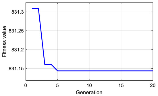
Figure 2. Fitness value of the 50 km/h constant radius test.

The GA-PSO is used to finally determine the TDC under different operating conditions of the vehicle, as shown in Table 2. To simplify the complexity of the table, the target yaw rate is expressed as the steady-state FWSA with equal torque distribution (ETD).

Table 2. Torque distribution coefficient of 10–80 km/h $\left[k,k_f,k_r\right]$.

FWSA of Equal Torque (deg)	Vehicle Speed (km/h)
	10	20	…	70	80
1	[0.7836,0.4377,0.2216]	[0.6451,0.4957,0.2305]	…	[0.7044,0.2799,0.2979]	[0.8512,0.4347,0.1758]
3	[0.7630,0.4130,0.3069]	[0.7581,0.4325,0.2001]	…	[    1    ,0.2273,     -     ]	[         ,0.2722,     -     ]
5	[0.8666,0.3516,0.4099]	[0.8617,0.3979,0.2959]	…	[0.9371,0.3264,0.4155]	-
7	[0.8832,0.3161,0.3768]	[    1    ,0.4227,     -     ]	…	-	-
…	…	…	…	…	…
27	[    1    ,0.2271,     -     ]	[    1    ,0.3994,     -     ]	…	-	-
29	[    1    ,0.2134,     -     ]	-	…	-	-

The corresponding target yaw rate and steady-state steering wheel angle can be obtained by using the steady-state FWSA with ETD in the first column of Table 2 so as to get the table of OTDC with minimum turning energy consumption. Table 2 illustrates that vehicles are gradually transitioned into a driving mode with front axle drive with the increase in steady-state FWSA with ETD, that is, $k = 1$. Meanwhile, it increases so gradually that the degree of torque transfers from the inside to the outside, that is, $k_f$ and $k_r$ gradually reduce. However, when the vehicle is approaching the extreme steering position, the torque distribution coefficient ($k_f$ & $k_r$) may increase slightly. Meanwhile, as the torque is transferred, the slip rate of the outside wheels will gradually increase. Therefore, from the perspective of reducing the energy consumption in wheel slip, the torque during the turning process of the vehicle cannot transfer without limitation.

Taking the simulation situation of a vehicle speed of 30 km/h, for example, the changes of vehicle motion state and energy consumption with or without the OTD are shown in Figure 3a–d. Figure 3a illustrates that the inner FWSA difference gradually increases with the increase in steady-state FWSA with ETD. Figure 3b illustrates that the yaw rate is almost unchanged after OTD, indicating that the characteristics of curve conditions of the vehicle are the same, and the vehicle can maintain its driving stability. It can be seen from Figure 3c that with the increase in the FWSA, the difference of the required power of the vehicle also gradually increases after OTD. Figure 3d shows that, as the FWSA increases, the energy conservation ratio (ECR) also gradually increases.

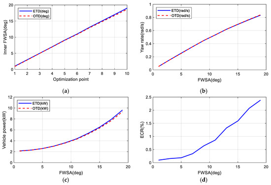
Figure 3. Curves of optimal torque distribution at 30 km/h: (a) inner FWSA; (b) yaw rate; (c) vehicle power; (d) energy-efficient ratio.

Figure 4 shows the energy-saving effect after a large number of simulation optimization tests obtained after a vehicle speed of 10 km/h–80 km/h and FWSA of 1°–29° were reached after OTD. According to the theoretical analysis in Section 3 of this article, the value of the turning resistance itself is not large when the speed of the vehicle and the FWSA are not large. Consequently, even if the TVD control is performed to reduce the turning resistance, the overall energy consumption of the vehicle is not significant. As the vehicle speed and FWSA increase, the turning resistance also gradually increases. Meanwhile, the TVD control of the vehicle will influence energy consumption a lot. It can be seen from the figure that the proportion of OTD energy saving increases gradually as the steering wheel angle and the vehicle speed increase. The highest energy-saving ratio of the model is 4.0415% in this article, the corresponding operating condition is the vehicle speed of 80 km/h, and the front wheel angle is about 4°.

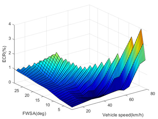
Figure 4. Energy-saving effect of optimal torque distribution.

5. Simulation Analysis of Torque Optimization Control Strategy Based on Motor Working Point

In this paper, the vehicle is driven by four hub motors. Accordingly, the power MAP of the motor will have a significant impact on energy saving in the actual application process.

5.1. Power Matching of Hub Motors

Considering the power requirements of the vehicle, it is necessary to match the four hub motors used in the vehicle. This article uses four identical hub motors to simplify the model. Referring to the power system matching of existing 4WID-EVs and vehicle dynamics indicators, the maximum required speed, maximum required torque, and peak power of the hub motor are matched so as to determine the hub motor that is suitable for the requirements of simulation and test of this article.

In consideration of the maximum speed, peak torque, and peak power of the vehicle under different operating conditions comprehensively, the selected hub motor MAP is shown in Figure 5. Its maximum speed is 1350 rpm, peak torque is 660 Nm, and peak power is 40 kW.

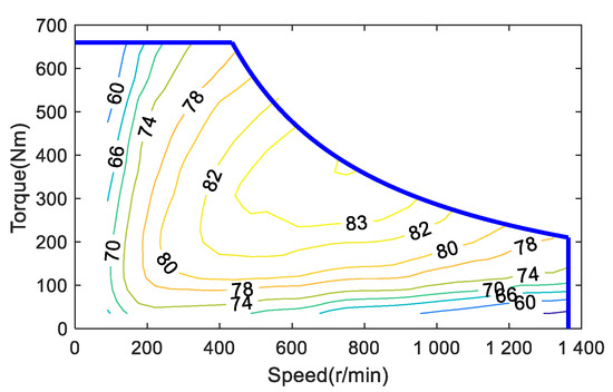
Figure 5. Motor efficiency map.

5.2. Selection of Optimal Torque Distribution Coefficient Based on Motor Working Point

In view of moto efficiency, the working point of the motor will change due to torque distribution, and the energy-saving ratio of corners change accordingly, as well. In order to achieve the best energy-saving contribution of torque distribution, we need to re-optimize the vehicle’s torque distribution coefficient (TDC, $k$, $k_f$ & $k_r$).

Using the GA-PSO described earlier in this article, we optimize respectively for the simulation conditions of vehicle speed at 10 km/h–80 km/h and front wheel angles of 1°–29° and finally get the TDC as shown in Table 3.

Table 3. Torque distribution coefficient based on working point at 10 km/h–80 km/h.

FWSA of Equal Torque (deg)	Vehicle Speed (km/h)
	10	20	…	70	80
1	[    1    ,    0    ,    -    ]	[    1    ,    0    ,    -    ]	…	[      0    ,    -    ,    0      ]	[0.3158,0.3363,0.4353]
3	[    1    ,    0    ,    -    ]	[    1    ,    0    ,    -    ]	…	[      1    ,    0    ,    -      ]	[     1    ,0.4800,    -     ]
5	[    0    ,    -    ,    0    ]	[    0    ,    -    ,    0    ]	…	[0.0509,0.2277,0.4832]	-
7	[    1    ,    0    ,    -    ]	[    1    ,    0    ,    -    ]	…	-	-
…	…	…	…	…	…
27	[    1    ,    0    ,    -    ]	[    1    ,    0    ,    -    ]	…	-	-
29	[    1    ,    0    ,    -    ]	[    1    ,    0    ,    -    ]	…	-	-

From the table above, the changes in the TDC of the vehicle are very obvious comparing with Table 2 in the previous section. Most vehicle working modes are front-axle drive and outer-wheel drive, especially in the corners of low and medium speeds and small front wheel corners when considering the impact of the motor working point on energy consumption.

Taking a turning condition with a vehicle speed of 30 km/h and a front wheel angle of 11° as an example, the motor working point of ETD and OTD is shown in Figure 6 and Figure 7. Since the current total torque demand of the vehicle is not large, the efficiency of the motor working point of ETD is about 72%. When the vehicle is with OTD, on the one hand, it is hoped that the larger the driving torque difference between the outer wheels and the inner wheels, the better the energy-saving effect of the vehicle; on the other hand, the higher the efficiency of the motor operating point, the better the energy-saving effect of the vehicle. Considering the two factors comprehensively, increasing the torque of the outer wheel and the motor working point will move to a more efficient point. Reduce the torque of the inner wheel, and the motor operating point will move lower. Without considering other power losses of the motor, it is believed that the vehicle is only driven by the outer wheels, which has the best effect on weakening the turning resistance. At the same time, torque is distributed in the outer wheels of the front and rear axles. Since the total torque demand of the motor at this time is not large and is only driven by a single motor, the efficiency of the motor working point will be higher. Therefore, it is believed that the vehicle driven by a single outer wheel has the highest contribution to energy saving, considering the influence of the TVD control and the motor working point. In combination with Table 3, as the total required torque of the vehicle is not large, to improve the energy-saving contribution of the TVD control to the vehicle’s curve conditions, most of its driving mode is single outer-wheel drive. This feature is conspicuous in the low-to-medium speed and small turning radius conditions.

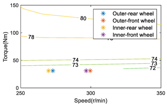
Figure 6. Working point of equal torque distribution at 30 km/h.

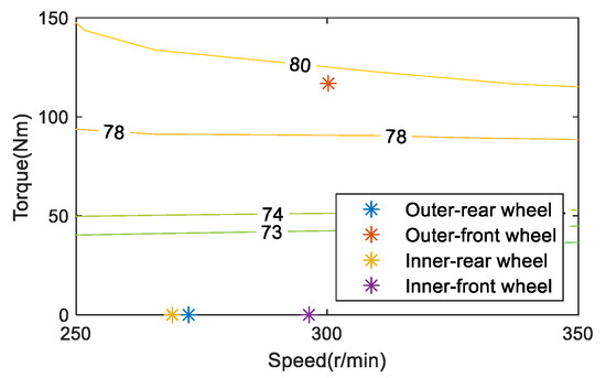
Figure 7. Working point of optimal torque distribution at 30 km/h.

If the working points of the four hub motors in corners are all in the low-efficiency zone, a single outer front-wheel drive model can be adopted to the maximum extent so as to improve the contribution of the TVD to the energy saving of the vehicle. It can simplify the complexity of offline optimization and shorten the optimization time while ensuring vehicle stability.

Figure 8 presents the energy-saving effect after a large number of simulation optimization experiments with a vehicle speed of 10 km/h–80 km/h and FWSA of ETD of 1°–29°. In Figure 8, the higher the color temperature of the box, the higher its contribution to energy saving. The figure indicates that the contribution of TVD control to the energy-saving of the vehicle is significantly improved, taking the change of the motor working point into account. For the vehicle model and motor model described in this article, the highest energy-saving ratio is 19.1107%, and the corresponding operating condition is the vehicle speed of 70 km/h and a front wheel angle of about 3°.

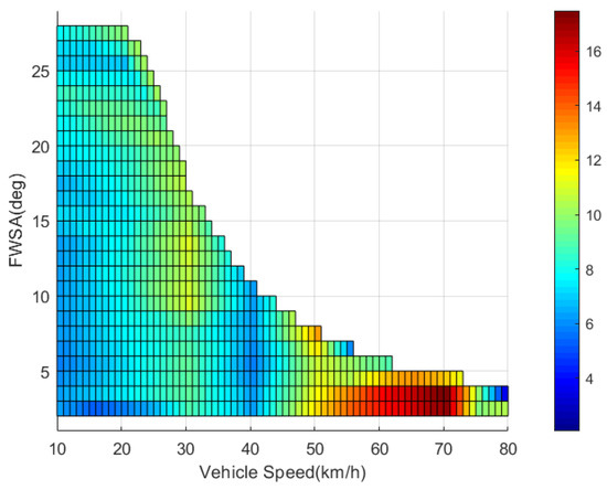
Figure 8. Energy-saving effect based on motor working point.

The comparison of Figure 4 with Figure 8, invites consideration of whether the influence of the motor working point will make a very big difference in the energy-saving contribution of the OTD control to the entire vehicle. The highest contribution of energy saving is only 4% without considering the motor working point. With the motor working point, it is 19%. The energy-saving contribution of each turning condition is much higher than the value in Figure 4. In addition, in comparing the trend of energy-saving contributions in the two pictures of the same vehicle speed and different front wheel angles, it can be seen that the energy-saving contribution has an obvious linear increasing trend when only the vehicle dynamics model is considered, and there is no obvious similar feature presented in Figure 8. Meanwhile, in comparing the changing trend in the two pictures of the energy-saving contribution of the same FWSA at different speeds, the energy-saving contribution has a clear parabola increasing trend only considering the vehicle dynamics model, and this feature in Figure 8 is also not obvious.

From the comparison of the results in the simulation analysis of Section 4 and Section 5, the influence of the change of the motor working point on the energy-saving contribution of the vehicle is significant and cannot be ignored. Therefore, when matching different motors to the vehicle, the final energy-saving effect will exhibit obvious differences.

6. Hardware-in-the-Loop Test Verification

This study developed the test conditions of a lemniscate-shape path as shown in Figure 9 and used the dSPACE real-time simulation system, then defined the test vehicle speed of 40 km/h and the initial vehicle speed of 40 km/h. The vehicle travels clockwise from the point (0,0), turning left and then right.

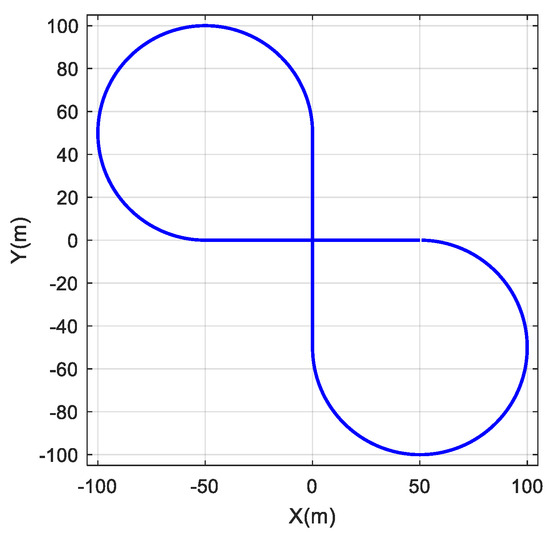
Figure 9. Lemniscate–shape path.

The change of vehicle speed during the test is presented in Figure 10. The vehicle speed always fluctuates up and down 40 km/h due to the driver’s manipulation, since the accelerator pedal signal of the driving simulator used in this article is very sensitive. Slight changes will cause obvious fluctuations in the speed of the vehicle, making it difficult to compare the test results. Therefore, this chapter selects the test segments of almost the same speed at 5–10 s to make key points.

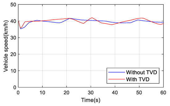
Figure 10. Curves of vehicle speed.

The change of steering wheel angle during the test is shown in Figure 1. To avoid the frequent adjustment of torque by TVD control, which affects the driver’s driving experience, the adjustment range of steering wheel angle is −10°–10°, where TVD does not work. Figure 11 illustrates that the steering angle of the steering wheel with TVD control is slightly smaller. The change of the yaw rate is shown in Figure 12. It can be seen that there is a slight deviation of the yaw rate with TVD control due to the driver’s operating. However, we also know that the yaw rate remains basically unchanged and is always able to maintain the driving stability of the vehicle.

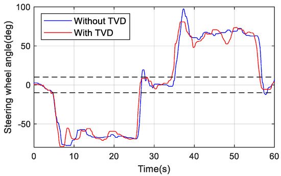
Figure 11. Curves of steering wheel angle.

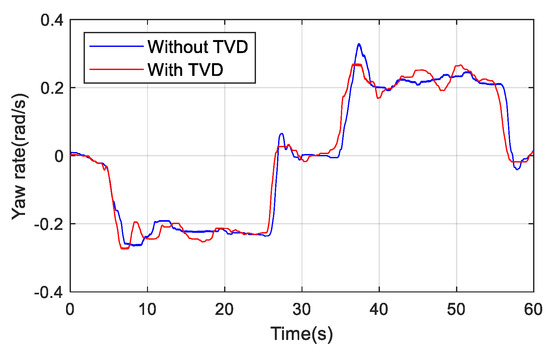
Figure 12. Curves of yaw rate.

The change of the power is shown in Figure 13.

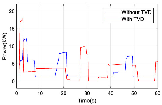
Figure 13. Curves of power.

This section may be divided by subheadings. It should provide a concise and precise description of the experimental results, their interpretation, and the experimental conclusions that can be drawn.

7. Conclusions

After the theoretical derivation of the 3-DOF vehicle dynamics model and the analysis of the longitudinal force change of the vehicle in turning, the influence of the TVD on the reduction in the vehicle turning energy consumption was described in this paper. Then, an optimal torque control strategy with a minimum turning energy consumption, including the economy and stability comprehensively, was proposed. Taking vehicle speed and yaw rate as control targets, the model uses GA-PSO to optimize the torque distribution coefficient offline. Lastly, the table of torque distribution coefficients for the minimum turning energy consumption was developed, which is based on the vehicle dynamics model and the best energy-saving contribution of torque distribution control under different turning conditions. Simulation results showed that the proposed optimal torque control strategy can reduce vehicle-turning energy consumption by 4% according to the vehicle dynamic model established in this paper.

In practical application, the influence of motor working point on torque distribution coefficient should be further considered. A more advanced table based on the motor working point was worked out. The influence of the motor working point on the best energy-saving contribution was illustrated by simulation experiment. Simulation analysis indicated that the improved strategy can reduce turning energy consumption by up to about 19%. Moreover, a simplified driving mode preliminarily of “front axle-drive, outer wheel-drive,” which can be adopted for low and medium speeds and small turning radius conditions in practical application, was also proposed so as to simplify the steps and reduce the difficulty of optimization control.

Finally, with the hardware-in-the-loop test, it has been proven that the optimal torque control strategy can effectively reduce vehicle turning energy consumption, on the premise of maintaining the stability of the vehicle. The accuracy and feasibility of the control strategy proposed were verified. However, further study related to the energy consumption and stability of vehicle cornering in the prospective research process need to be done so as to realize the online correction and coordinated control of the energy saving and stability of EVs.

References

- Wang, J.; Wang, Q.; Jin, L.; Song, C. Independent wheel torque control of 4WD electric vehicle for differential drive assisted steering. Mechatronics 2011, 21, 63–76. [Google Scholar] [CrossRef]
- Wang, J.; Yang, B.; Wang, Q.; Jiantu, N.I. Review on Vehicle Drive Technology of Torque Vectoring. J. Mech. Eng. 2020, 56, 92. [Google Scholar]
- Liu, J.; Zhuang, W.; Zhong, H.; Wang, L.; Chen, H.; Tan, C.-A. Integrated energy-oriented lateral stability control of a four-wheel-independent-drive electric vehicle. Sci. China Technol. Sci. 2019, 62, 2170–2183. [Google Scholar] [CrossRef]
- Oh, K.; Joa, E.; Lee, J.; Yun, J.; Yi, K. Yaw Stability Control of 4WD Vehicles Based on Model Predictive Torque Vectoring with Physical Constraints. Int. J. Automot. Technol. 2019, 20, 923–932. [Google Scholar] [CrossRef]
- Park, J.-Y.; Heo, S.-J.; Kang, D.-O. Development of Torque Vectoring Control Algorithm for Front Wheel Driven Dual Motor System and Evaluation of Vehicle Dynamics Performance. Int. J. Automot. Technol. 2020, 21, 1283–1291. [Google Scholar] [CrossRef]
- Koehler, S.; Viehl, A.; Bringmann, O.; Rosenstiel, W. Improved energy efficiency and vehicle dynamics for battery electric vehicles through torque vectoring control. In Proceedings of the 2015 IEEE Intelligent Vehicles Symposium (IV), Seoul, Korea, 28 June–1 July 2015; IEEE: Piscataway, NJ, USA, 2015; pp. 749–754. [Google Scholar]
- Wang, J. Study on Differential Drive Assist Steering for Electric Vehicle with Independent-Motorized-Wheel-Drive. Ph.D. Thesis, Jilin University, Changchun, China, 2009. [Google Scholar]
- Alipour, H.; Sabahi, M.; Sharifian, M.B.B. Lateral stabilization of a four wheel independent drive electric vehicle on slippery roads. Mechatronics 2015, 30, 275–285. [Google Scholar] [CrossRef]
- Wang, J.; Yu, T.; Sun, N.; Fu, T. Torque Vectoring Control of Rear-Wheel-Independent-Drive Vehicle after Cornering Efficiency Improvement. J. Hunan Univ. (Nat. Sci.) 2020, 47, 9–17. [Google Scholar]
- Yu, S.; Li, W.; Liu, Y.; Chen, H. Steering Stability Control of Four-Wheel-Drive Electric Vehicle. Control. Theory Appl. 2021, 38, 12. [Google Scholar]
- Sun, W.; Wang, J.; Wang, Q.; Assadian, F.; Fu, B. Simulation investigation of tractive energy conservation for a cornering rear-wheel-independent-drive electric vehicle through torque vectoring. Sci. China Technol. Sci. 2018, 61, 257–272. [Google Scholar] [CrossRef]
- Wong, A.; Kasinathan, D.; Khajepour, A.; Chen, S.K.; Litkouhi, B. Integrated torque vectoring and power management framework for electric vehicles. Control. Eng. Pract. 2016, 48, 22–36. [Google Scholar] [CrossRef]
- Andrzej, S.; Ireneusz, P.; Wojciech, C. Fuel Cell Electric Vehicle (FCEV) Energy Flow Analysis in Real Driving Conditions (RDC). Energies 2021, 14, 5018. [Google Scholar]
- Serpi, A.; Porru, M. Modelling and Design of Real-Time Energy Management Systems for Fuel Cell/Battery Electric Vehicles. Energies 2019, 12, 4260. [Google Scholar] [CrossRef]
- Mariusz, I.; Marianna, J. An Efficient Hybrid Algorithm for Energy Expenditure Estimation for Electric Vehicles in Urban Service Enterprises. Energies 2021, 14, 2004. [Google Scholar]
- Irfan, U.; Liu, K.; Toshiyuki, Y.; Muhammad, Z.; Arshad, J. Electric vehicle energy consumption prediction using stacked generalization: An ensemble learning approach. Int. J. Green Energy 2021, 18, 896–909. [Google Scholar]
- Pierpaolo, P.; Ivan, A.; Cesare, P. Optimal Energy Management for Hybrid Electric Vehicles Based on Dynamic Programming and Receding Horizon. Energies 2021, 14, 3502. [Google Scholar]
- Rossa, F.D.; Mastinu, G.; Piccardi, C. Bifurcation analysis of an automobile model negotiating a curve. Veh. Syst. Dyn. 2012, 50, 1539–1562. [Google Scholar] [CrossRef]
- Inagaki, S.; Kushiro, I.; Yamamoto, M. Analysis on Vehicle Stability in Critical Cornering Using Phase-Plane Method. JSAE Rev. 1995, 16, 216. [Google Scholar]
- Wang, J. Steering Stability Control of Four-Wheel Drive Vehicle with Hub Motors. M.D. Thesis, Beijing Institute of Technology, Beijing, China, 2015. [Google Scholar]
- Ando, K.; Sawase, K.; Takeo, J. Analysis of tight corner braking phenomenon in full-time 4WD vehicles. JSAE Rev. 2002, 23, 83–87. [Google Scholar] [CrossRef]
- Sun, W.; Wang, Q.N.; Wang, J.N. Yaw-moment control of motorized vehicle for energy conservation during cornering. Jilin Daxue Xuebao/J. Jilin Univ. 2018, 48, 11–19. [Google Scholar]
- Slowik, A. Application of evolutionary algorithm to design minimal phase digital filters with non-standard amplitude characteristics and finite bit word length. Bull. Pol. Acad. Sci. Tech. Sci. 2011, 59, 125–135. [Google Scholar] [CrossRef][Green Version]
- Wen, Z.; Liu, Y. Reactive power optimization based on PSO in a practical power system. In Power Engineering Society General Meeting; IEEE: Piscataway, NJ, USA, 2004. [Google Scholar]
- Bakare, G.A.; Chiroma, I.N.; Venayagamoorthy, G.K. Comparison of PSO and GA for K-Node Set Reliability Optimization of a Distributed System. In Proceedings of the 2006 IEEE Swarm Intelligence Symposium, Indianapolis, IN, USA, 12–14 May 2006. [Google Scholar]
- Roberge, V.; Tarbouchi, M.; LaBonte, G. Comparison of Parallel Genetic Algorithm and Particle Swarm Optimization for Real-Time UAV Path Planning. IEEE Trans. Ind. Inform. 2012, 9, 132–141. [Google Scholar] [CrossRef]
- Liu, J.C.; Chen, Y.Z. A BPNN-Based Speed Prediction Method with GA-PSO Optimization Algorithm. J. Transp. Syst. Eng. Inf. Technol. 2017, 17, 40–47. [Google Scholar]
- Gao, Y.; Zhang, R. A network traffic prediction based on bp neural network optimized by a GA-PSO algorithm. Comput. Appl. Softw. 2014, 31, 106–110. [Google Scholar]
Publisher’s Note: MDPI stays neutral with regard to jurisdictional claims in published maps and institutional affiliations. |
© 2021 by the authors. Licensee MDPI, Basel, Switzerland. This article is an open access article distributed under the terms and conditions of the Creative Commons Attribution (CC BY) license (https://creativecommons.org/licenses/by/4.0/).