Abstract
Shared mobility based on cars refers to a transportation mode in which travelers/drivers share vehicles to reduce the cost of the journey, emissions, air pollution and parking demands. Cost savings provide a strong incentive for the shared mobility mode. As cost savings are due to cooperation of the stakeholders in shared mobility systems, they should be properly divided and allocated to relevant participants. Improper allocation of cost savings will lead to dissatisfaction of drivers/passengers and hinder acceptance of the shared mobility mode. In practice, several schemes based on proportional methods to allocate cost savings have been proposed in shared mobility systems. However, there is neither a guideline for selecting these proportional methods nor a comparative study on effectiveness of these proportional methods. Although shared mobility has attracted much attention in the research community, there is still a lack of study of the influence of cost saving allocation schemes on performance of shared mobility systems. Motivated by deficiencies of existing studies, this paper aims to compare three proportional cost savings allocation schemes by analyzing their performance in terms of the numbers of acceptable rides under different schemes. We focus on ridesharing based on cars in this study. The main contribution is to develop theory based on our analysis to characterize the performance under different schemes to provide a guideline for selecting these proportional methods. The theory developed is verified by conducting experiments based on real geographical data.
1. Introduction
Energy consumption and the associated impact on the environment due to urbanization and growth of population are two challenges directly linking to sustainability of cities that have attracted researchers’ attention for decades. According to [1], the transportation sector accounts for a large proportion of global energy consumption and greenhouse gas (GHG) emissions. Fuel combustion in the transportation sector accounts for 24% of direct CO2 emissions, which has significant impact on the environment. How to effectively minimize the impact on the environment by the transportation sector is critical to achieve sustainability of cities. Sharing economy has attracted much attention of practitioners, researchers, policy makers and individuals to improve efficiency and sustainability based on sharing of assets [2]. The transportation sector contributes to a large part of energy consumption and hence the study on green transportation and solutions has become an important research subject for the sustainable development of sharing economy [3]. In the past years, shared mobility emerges as a popular transportation mode that attracts the attention of researchers as well as practitioners in the transportation sector [4]. Shared mobility refers to a transportation mode in which travelers/drivers share vehicles to reduce the cost of the journey, energy consumption, emissions, air pollution and parking demands. It takes different forms in the world, including ridesharing, carpooling and bike sharing [5,6]. In this paper, we consider ridesharing systems based on cars. Shared mobility services enable users to access transportation services conveniently on an as-needed basis. Thus, shared mobility services provide a flexible transportation option besides public transport. In addition to the advantage due to flexibility in terms of routing and timing, users of shared mobility services also can enjoy the benefits of cost savings due to the shared use of vehicles.
Cost savings provide a strong incentive for the shared mobility mode. Therefore, optimization of performance metrics relevant to cost savings in shared mobility systems has been extensively studied in the literature [7,8,9]. As the primary incentive for users to share a ride is cost savings, the way to allocate cost savings is an important factor to the adoption of ridesharing by the users. Allocation of a portion of cost savings to the service providers is also important for maintaining operation of ridesharing information systems. As cost savings are due to cooperation of the stakeholders in shared mobility systems based on cars, they should be properly divided and allocated to relevant participants. In the literature, several schemes to allocate costs/cost savings among players in a coalition of transportation systems have been studied in [10]. Due to computational complexity and the need for agile problem solvers [8], proportional methods have been adopted in practice to allocate costs/cost savings. For ridesharing systems, several schemes to allocate cost savings have been proposed based on proportional methods, e.g., [11,12,13]. However, there is no guideline to select the correct and proper scheme for allocation of cost savings due to the lack of a comparative study on these proportional schemes. Improper allocation of cost savings will discourage users and hinder acceptance of the shared mobility model. This is due to the lack of consideration of the satisfaction factor of drivers and passengers. For example, suppose all cost savings are allocated to the passengers. The drivers will not accept share rides with passengers. Therefore, how to allocate cost savings properly is an important issue. Although proportional methods have been proposed and studied in different problem domains [10], analysis of effectiveness of the three proportional allocation methods for ridesharing has not been carried out. Although shared mobility has attracted much attention in the research community, there is still a lack of study on the influence of cost savings allocation schemes on the performance of shared mobility systems. Motivated by deficiencies of existing studies on these issues, this paper aims to develop a framework to compare the three different cost savings allocation schemes proposed in [11,12,13] based on proportional methods and compare their performance in terms of the numbers of acceptable rides under different schemes. The contributions of this paper are three-fold. First, we develop theory to compare the performance of the three different cost savings allocation schemes. Second, we provide a guideline with rules for selecting a proper cost savings allocation scheme from the three cost savings allocation schemes for shared mobility systems. Third, policy makers may apply the guideline to increase the number of acceptable shared rides to enhance sustainability and service providers may apply the guideline to increase the number of acceptable shared rides and profits.
The decision support systems for shared mobility systems with cars typically include two stages—stage 1: determination of shared rides and stage 2: allocation of cost savings [13]. For the drivers and passengers, they must make decisions about whether they accept the recommended rides for ridesharing. In this paper, we assume that the drivers and passengers determine whether to accept shared rides based on the minimal expected rewarding rate. A ride recommended by the decision support systems for shared mobility systems with cars accepted by the driver and the passenger is called an acceptable ride. The stakeholders include drivers, passengers and the shared mobility service/information provider. Schemes to allocate cost savings to the stakeholders in shared mobility systems are defined based on these stakeholders. To achieve the goals of this paper, there are four tasks to complete: (1) identification of shared mobility decision model and definition of schemes to allocate cost savings to participants, (2) introduction of the concept of minimal expected rewarding rate of drivers and passengers and development of theory based on analysis of the influence of different cost savings allocation schemes on the number of acceptable shared rides, (3) verification of the developed theory by test cases and (4) a guideline for selecting the proper proportional scheme to allocate cost savings.
The structure of the remainder of this paper follows. In Section 2, we briefly review existing studies on shared mobility systems with cars. In Section 3, a shared mobility decision model and the three proportional schemes, including Fifty-Fifty Scheme, Local Proportional Scheme and Global Proportional Scheme, to allocate cost savings to the stakeholders in shared mobility systems are defined. We compare the Fifty-Fifty Scheme and Local Proportional Scheme in Section 4, compare the Local Proportional Scheme and Global Proportional Scheme in Section 5 and compare the Global Proportional Scheme and Fifty-Fifty Scheme in Section 6. We verify theoretical properties by examples in Section 7. In Section 8, we provide a discussion based on the results obtained and, to allocate cost savings, offer a guideline for selecting a proper proportional scheme from the three schemes studied in this paper. Finally, we conclude this paper in Section 9.
2. Literature Review
The widespread adoption of mobile communication devices and ICT to provide efficient access to transportation services has made shared mobility an important paradigm for cities [14]. Shared mobility may take different forms, including sharing of vehicles and sharing of rides [15]. The former allows cars, motorcycles, scooters, and bikes to be shared and the latter enables ridesharing and on-demand ride services for passenger rides. The benefits of shared mobility include significant reduction of total travel distance, trip cost, carbon emissions and congestion [16,17]. The advantages of ridesharing lead to several variants of transportation modes. Carpooling is an early variant of ridesharing in which employees in companies are encouraged to travel with colleagues for commuting to minimize the number of cars traveling to sites of the companies and travel cost of the employees [18]. Vanpooling is another variant of ridesharing transportation mode. In vanpooling, commuters drive to an intermediate location to take a van and ride together to the destination [19]. Generally speaking, ridesharing reduces the travel cost for people with similar itineraries and schedules by sharing vehicles [5]. In addition, ridesharing models with mixed passengers, parcels [20] or goods [21] were proposed. Recent trends in studies on ridesharing include social ridesharing, such as the one in presented in [22].
In this paper we focus on ridesharing systems with cars. Although shared mobility promises to achieve sustainability of cities, reduce energy consumption and provide an alternative way to meet passengers’ transportation need without owning a car, it relies on the development of an efficient decision model and decision support tools to attain these goals. Actually, shared mobility poses several challenging research issues [7,8,23]. In the literature, optimization of shared mobility systems was discussed in [7,8]. The solution algorithms can be classified into exact methods and heuristic/metaheuristic methods. Exact methods are applied to find the optimal solutions for optimization of shared mobility systems [24]. Exact methods, however, can only be applied to small problems due to computational complexity. Therefore, many heuristic/metaheuristic methods have been proposed to solve optimization problems of shared mobility systems. For example, the genetic algorithm [25], tabu search [26], population-based metaheuristic algorithms [27], the differential evolution algorithm [28] and hybridization of metaheuristics [29] have been proposed to solve relevant optimization problems in shared mobility systems.
Beside optimization issues, efforts to realize shared mobility have developed. Mobility-as-a-service (MaaS) aims to provide users access to shared mobility services through a single friendly online interface from planning, booking to payment. Several cities have already implemented or are in the process of implementing MaaS trials or pilot projects. Although MaaS provides a potential alternative to private vehicle ownership, there are barriers and risks for adoption of MaaS in cities [30] such as the lack of appeal to public transport users and private vehicle users. Ridesharing is a potential transportation mode to reduce the number of cars, but it is still not widely adopted. Studies in [31,32] point out that savings of cost and time are the main incentives for ridesharing. For ridesharing drivers and passengers, a proper scheme to allocate cost savings among participants is important for adoption of ridesharing.
In the literature, the problem to allocate costs/cost savings among players in a coalition of transportation systems has been studied in [10]. Shapley value [33], nucleolus [34] and proportional methods [35] have been proposed in the literature to allocate costs/cost savings in cooperative game theory. Shapley value [33] and nucleolus [34] suffer from computational complexity problems [36,37]. Therefore, proportional methods [35] are often adopted in practice. There are many studies on application of proportional methods in different domains in the literature. For example, a pricing scheme is used in [38] is to maximize the total profit through exchanging transportation requests among collaborative carriers. In [39], proportional methods are used to allocate costs and emissions in a carrier’s delivery network with multiple customers served by a single carrier. As transportation cost of low-value forest fuels, including trees, tree bark, branches, stumps and wood chips, accounts for a large part in logistic cost, several alternative ways applying proportional methods to lower logistic cost of forest fuels transport have been studied in [40].
In the context of ridesharing systems, several cost allocation methods have been developed. The problem to achieve fair cost allocation in ridesharing systems based on the nucleolus method has been studied in [41]. In [42], the problem to allocate passengers to drivers, charge passengers and create feasible schedules for drivers in a dynamic ridesharing scenario is addressed. Due to computational complexity and the need for agile algorithms in ridesharing systems, proportional methods have been widely used in practice. For example, the ones proposed in [11,12,13] are based on proportional methods. In [11], the authors consider a ridesharing problem in which each driver shares a ride with at most one rider. The cost allocation scheme proposed in [11] divides the cost savings of sharing a ride equally between the two matched participants (the driver and the rider) of the shared ride. Such cost allocation satisfies the property of Shapley value in the cooperative game theory. In [12], the authors considered ridesharing systems in which at most one pickup and delivery may take place during the trip and transfers are not allowed. In [12], it is assumed that costs are proportional to vehicle-miles driven. The cost savings allocated to the driver and the rider are proportionally to the lengths of their original trips. The cost allocation schemes in [11,12] are proposed for ridesharing systems in which each shared ride includes one driver and one rider. In [13], a ridesharing problem which allows multiple passengers to be transported by a driver is considered. A cost allocation scheme which divides the cost savings among three types of stakeholders in a ridesharing system, including ridesharing information provider, drivers and riders, is proposed. The cost savings allocation scheme proposed in [13] allocates a portion of the overall cost savings to the ridesharing information provider and the remaining cost savings to each ridesharing passenger and each driver, which is based on the weighting of their bid price with respect to overall bid price of all ridesharing passengers’ and all drivers’ bids. However, there still lacks a comparative study on whether the cost savings allocated by these allocation schemes are acceptable for drivers and passengers. That is, the cost savings allocation schemes will surely influence the number of acceptable shared rides for drivers and passengers. An interesting but unexplored research issue is to compare the number of acceptable rides that can be satisfied under the three proportional cost savings allocation schemes proposed in [11,12,13].
This paper does not focus on optimization of the ridesharing matching problems to minimize overall travel distance or maximize overall cost savings. In this paper, we will study effectiveness of three cost savings allocation schemes in terms of the number of acceptable shared rides that satisfy the minimal rewarding rate requirements of drivers and passengers. In the literature, different ridesharing matching methods have been proposed. To ensure fairness of comparison, the overall cost savings of a ridesharing system are obtained by the same ridesharing matching method. The cost savings allocation policies to be compared in this paper include those proposed in [11,12,13]. We compare the three cost savings allocation schemes by theoretical analysis. The properties and theorems established through analysis are verified by examples.
3. Decision Model and Cost Savings Allocation Schemes for Shared Mobility Systems
The decision support systems for shared mobility systems typically include two decision stages. A decision model for shared mobility systems is used in the first stage to find the shared rides. In the second stage, the solution obtained from the decision model is then used to divide the cost savings among the participants by applying different allocating schemes. To focus on the comparison of different schemes for allocating cost savings, the decision model in [13] based on maximization of cost savings will be used in this study. A list of notations used in this study is summarized in Table 1 for reference.

Table 1.
Notations of symbols, variables and parameters.
3.1. Decision Model
The decision support system for ridesharing makes decisions within a time period. Requests of drivers and passengers arriving before the start of the decision time period will be considered by the ridesharing decision support system. The decision support system follows the framework in [13] and the decision period is divided into two stages—stage 1: determination of shared rides and stage 2: allocation of cost savings. In the decision model used in stage 1, drivers and passengers submit bids [13]. Bids are generated by bid generation procedures to meet spatial, time and capacity requirements/constraints of drivers and passengers. The bid generation procedure for passengers generates bids based on the origins, destinations, earliest departure time, latest arrival time and number of seats requested by passengers. The bid generation procedure for drivers generates bids based on the origins, destinations, earliest departure time, latest arrival time, the number of seats for ridesharing and the maximum detour ratio specified by drivers. Therefore, the decision model can handle spatial, time and capacity requirements in ridesharing systems. In addition, the decision model is flexible and has been extended in [22] to deal with trust requirements in social ridesharing problems.
For the above decision model, suppose passengers and drivers submit bids to the systems. The bid of passenger is = , where is the number of seats requested for passenger ’s pick-up location, is the number of seats released at passenger ’s drop-off location and is the cost of passenger without ridesharing. A driver may submit multiple bids, but only one bid can be accepted. A bid accepted by the system is called a winning bid. = denotes the bid of driver , where is the number of seats allocated at passenger ’s pick-up location, is the number of seats released at passenger ’s drop-off location, is the cost when the driver travels alone and is the cost of the bid. It is assumed that the bids of passengers and drivers are generated by applying bid generation procedures developed in [13], taking into account the timing, capacity and spatial constraints of drivers and passengers. The bid generation procedures calculate the cost based on a function , where is the travel distance. The decision model in [13] can handle the bids regardless of whether the function used to calculate cost is linear or nonlinear.
The overall cost savings are the difference between the overall original cost (without ridesharing) and the overall cost after ridesharing. Original cost of passengers (without ridesharing) and original cost of drivers (without ridesharing) is . Cost of passengers and drivers with ridesharing is . The overall cost savings are the difference between these two terms. That is, the overall cost savings are .
The decision problem aims to determine the winning bids submitted by the potential drivers and passengers to maximize the overall cost savings. Thus, the objective function is defined in (1) as follows:
The problem to determine the winning bids is formulated as an integer programming problem subject to demand and supply constraints (2), (3), nonnegative cost savings constraint (4) and single winning bid constraints for drivers (5) as follows:
s.t.
Due to computational complexity, only small instances of the above problem can be solved by applying exact algorithm due to exponential growth of solution space with respect to the problem size. In the literature, the problem to optimize cost savings in ridesharing systems has been extensively studied. Many approximate approaches can be applied to solve this problem, including evolutionary computation algorithms, bio-inspired evolutionary algorithms and metaheuristic approach. Therefore, many algorithms have been proposed to solve this problem, e.g., [13,28]. A comparison of these approaches appears in the literature [13]. The comparative study provides a guideline for selection of a solution methodology for solving the above cost savings optimization problem. As this paper focuses on comparison of cost allocation schemes, it is assumed that a solution algorithm is used to solve the cost savings optimization problem in the shared mobility model to ensure fairness in comparison of different cost allocation schemes. In this paper, the algorithm proposed in [13] is applied to determine the winning bids.
3.2. Three Cost Savings Allocation Schemes Based on Proportional Methods
Cost savings in ridesharing systems are due to collaboration of the participants in shared rides. Ridesharing can be considered as a type of collaborative transportation through which the participants, drivers and passengers in shared rides benefit from cost savings. Therefore, the participants in shared rides can be regarded as a coalition. The issue is to divide cost savings among participants in the coalition in collaborative transportation modes [10]. As cost savings are due to cooperation of participants in the coalition, they must be divided and allocated properly. Different ways to allocate cost savings can be developed for the shared mobility system. Several cost allocation methods have been proposed in the literature. Shared mobility systems can be modeled as a class of cooperative games in which participants represented by agents cooperate to benefit from cost savings. Consider a set = {1, …, N} of all players in a cooperative game. The set is called the “grand coalition.” For the set of all subsets of , we define a characteristic function : → to assign the cost to each coalition in . A cost allocation vector is denoted as = (,, …, ), which represents the value assigned to each player in . A cost allocation vector is also called a preimputation. The characteristic function and cost allocation vector satisfy the “efficiency” property if = 0 and . An allocation vector is said to be “rational” if there does not exist a subset of players such that they would perceive less total cost than the total cost allocated to them by forming a coalition separately from the rest. Rationality of an allocation vector can be represented by the constraints . The set of cost allocation vectors or preimputations satisfying rationality is called the “core”. An allocation in the core is stable as there is no subset of the players such that its players would be better off by deviating from the coalition.
Several well-known methods have been proposed to allocate cost. These include Shapley value [33], nucleolus [34] and proportional methods [35]. Each cost allocation method has its pros and cons. Two appealing features of Shapley value allocation are efficiency and uniqueness. However, Shapley value allocation does not belong to the core in general. In addition, Shapley value allocation poses a computation complexity challenge [33]. Nucleolus is more complex than Shapley value although it always belongs to the core [34]. A simple way for cost allocation is proportional methods [35]. In the literature, several schemes to allocate cost savings in ridesharing systems were proposed in [11,12,13] based on the proportional methods. However, a further study on application of the proportional methods to shared mobility systems is needed to assess effectiveness of these methods. In this section, the schemes proposed in [11,12,13] to allocate cost savings in shared mobility systems are defined. These schemes to allocate cost savings are analyzed in the next section.
A proportional method allocates a share of the total cost to each player . That is, , where . By assigning the share value properly, we can obtain the schemes proposed in [11,12,13].
In shared mobility systems, the players are the stakeholders, including the information provider, a set of passengers, and a set of drivers, . The share values for the information provider, passenger and driver are denoted by , and , respectively. Different cost savings allocation schemes can be defined by applying different rules to assign the share values , and , where . Instead of considering the original schemes proposed in [11,12,13] only, we generalize these schemes by taking into account allocation of cost savings to the information provider of shared mobility systems in addition to drivers and passengers. The three schemes proposed in [11,12,13] are variants of proportional methods defined by specifying the share values differently. For these three cost savings allocation schemes, it is assumed that the information provider is allocated of cost savings. Let us define these three schemes formally.
For the convenience of discussions, we will call the schemes proposed in [11,12,13] “Fifty-Fifty Scheme”, “Local Proportional Scheme” and “Global Proportional Scheme”, respectively. We call the scheme proposed in [11] “Fifty-Fifty Scheme” as the cost savings of sharing a ride are equally divided between the two matched participants (the driver and the passenger) of each shared ride under this scheme. That is, fifty percent of cost savings of a shared ride is rewarded to the driver and the remaining fifty percent of cost savings is rewarded to the passenger. We call the scheme proposed in [12] “Local Proportional Scheme” as it allocates the cost savings of a ride to the driver and the passenger proportionally to the lengths of their trips. We call the scheme proposed in [13] “Global Proportional Scheme” as it allocates the cost savings to the drivers and passengers based on the weighting of individual bid price with respect to overall bid price of all ridesharing passengers’ and drivers’ bids. These three schemes are formally defined next. As the original schemes proposed in [11,12,13] do not consider the portion of cost savings allocated to information provider, the “Fifty-Fifty Scheme”, “Local Proportional Scheme” and “Global Proportional Scheme” defined below extend the original schemes by taking into account allocation of cost savings to information provider. In each of the schemes, the cost savings are divided into three parts: the first part is allocated to the information provider, the second part is allocated to the drivers and the third part is allocated to the passengers.
The overall cost savings of a solution is clearly defined in (1). Before defining the three schemes, we first distinguish the cost savings of a single ride from overall cost savings. For the ride corresponding to a winning bid, say the -th bid submitted by driver , let denote the set of passengers in the ride corresponding to the -th bid submitted by driver . The cost savings of the -th bid submitted by driver is defined in (6) as follows:
The three schemes are defined as follows.
In the Fifty-Fifty Scheme, which considers one driver and one passenger of a shared ride, fifty percent of cost savings of the ride is rewarded to the driver and the remaining fifty percent of cost savings is rewarded to the passenger.
Definition 1.
Fifty-Fifty Scheme
- (1)
- This scheme allocatesto the information provider. The share value for the information provider is.
- (2)
- This scheme allocatesto the ridesharing passenger ( = 1) transported by driver , where . The share value for passenger ( = 1) is .
- (3)
- This scheme allocatesto each ridesharing driver( = 1 for some ), where . The share value for the ridesharing driver ( = 1 for some ) is .
Note that.
The scheme proposed in [12] allocates cost savings to the driver and the passenger proportional to the lengths of their trips. Let us call it the Local Proportional Scheme. The Local Proportional Scheme allocates to the information provider and allocates cost savings based on the weighting of the original bid price of each ridesharing passenger and driver in a shared ride with respect to overall bid price of the driver and the relevant passenger in the shared ride. The Local Proportional Scheme can be defined as follows:
Definition 2.
Local Proportional Scheme:
- (1)
- This scheme allocatesto the information provider. The share value for the information provider is.
- (2)
- This scheme allocatesto each ridesharing passenger ( = 1) transported by driver , where . The share value for the ridesharing passenger ( = 1) transported by driver is .
- (3)
- This scheme allocatesto each ridesharing driver ( = 1 for some ), where .
The share value for the ridesharing driver ( = 1 for some ) is
Note that.
The Global Proportional Scheme proposed in [13] allocates a portion of the overall cost savings to each participant according to the percentage of the participant’s travel cost with respect to the overall travel cost. The Global Proportional Scheme is different from the Local Proportional Scheme defined previously. This scheme allocates to the information provider and allocates the remaining cost savings to each ridesharing passenger and driver based on the weighting of their bid price with respect to overall bid price of all ridesharing passengers’ and drivers’ bids.
Definition 3.
Global Proportional Scheme:
- (1)
- This scheme allocatesto the information provider. The share value for the information provider is.
- (2)
- This scheme allocatesto the winning passenger ( = 1), where the share value .
- (3)
- This scheme allocatesto each winning driver ( = 1 for some ).
The share value for driver ( = 1 for some ) is
Note that.
To compare different cost savings allocation schemes, it is important to study how many matched rides can satisfy cost savings expectations for relevant drivers and passengers. We define the minimal expected rewarding rate as follows to describe the minimal cost savings expectations of drivers and passengers.
Definition 4.
The minimal cost savings expectations for a ridesharing participant (either a driver or a passenger) are called the minimal expected rewarding rate, which is defined as the ratio of the cost savings to the travel cost of the participant. The minimal expected rewarding rate is denoted by.
In the real world, drivers or passengers may not be satisfied with the shared rides recommended by the shared mobility system due to low rewarding rate even if these rides can meet their transportation requirements. A driver or a passenger may choose either to accept or reject a ride found by the ride matching system. To assess effectiveness of different schemes to allocate cost savings, we distinguish acceptable shared rides from unacceptable ones.
Definition 5.
A shared ride is an acceptable ride if the rewarding rate for all the participants on the ride is greater than or equal to the minimal expected rewarding rate. A shared ride is not an acceptable ride if the rewarding rate for any participant on the ride is less than the minimal expected rewarding rate.
We will compare effectiveness of the Fifty-Fifty Scheme, Local Proportional Scheme and Global Proportional Scheme by analyzing the number of acceptable rides.
4. Comparison of the Fifty-Fifty Scheme and Local Proportional Scheme
In this section, we will compare the Fifty-Fifty Scheme and Local Proportional Scheme by analysis. Based on the analysis, a theorem will be stated to characterize the relation of these two schemes in terms of the number of acceptable rides.
A passenger or a driver will not accept to share a ride if any of their minimal cost savings expectations, i.e., the minimal expected rewarding rate, cannot be met. A shared ride is called an acceptable ride if the rewarding rate of the driver and the rewarding rate of the passenger are greater than or equal to the minimal expected rewarding rate. The comparison between cost savings allocation schemes is based on the number of acceptable shared rides. We first state two lemmas to pave the way for the establishment of a theorem that state the relation between the number of acceptable rides under the Fifty-Fifty Scheme and Local Proportional Scheme.
Lemma 1.
Suppose the original travel distance of the passengeris not greater than that of the driveron a shared ride (with = 1 for some ). The rewarding rate for driver (with = 1) under the Fifty-Fifty Scheme is less than or equal to that under the Local Proportional Scheme. The rewarding rate for passenger in the shared ride is greater than or equal to the rewarding rate for driver .
Proof of Lemma 1.
Under the Fifty-Fifty Scheme, the cost savings allocated to driver in the ride corresponding to the -th bid of driver with = 1 is . The rewarding rate for driver is . Under the Local Proportional Scheme, the cost savings allocated to driver with = 1 is . The rewarding rate for driver with = 1 is . In [12], it is assumed that there is at most one passenger transported by a driver; there is only one element in . Let denote the passenger transported by driver . Then = = . As the original travel distance of the passenger is not greater than that of the driver in the shared ride, . Hence .
Therefore, .
In this case, the rewarding rate for driver with = 1 under the Fifty-Fifty Scheme is less than or equal to that under the Local Proportional Scheme.
Note that, as , .
Therefore, the rewarding rate for passenger in the ride corresponding to the -th bid of driver with = 1 is greater than or equal to the rewarding rate for driver . □
Lemma 2.
Suppose the original travel distance of passengeris greater than that of the driverin the shared ride corresponding to the-th bid of driverwith = 1. The rewarding rate for passenger under the Fifty-Fifty Scheme is less than that under the Local Proportional Scheme. The rewarding rate for driver in the shared ride is greater than the rewarding rate for passenger .
Proof of Lemma 2.
Under the Fifty-Fifty Scheme, the cost savings allocated to passenger is . The rewarding rate for passenger is . Under the Local Proportional Scheme, the cost savings allocated to passenger is .
The rewarding rate for passenger is . In [12], it is assumed that there is at most one passenger transported by a driver; there is only one element in . Let denote the passenger transported by driver . Then = = .
As , .
Hence . In this case, the rewarding rate for passenger under the Fifty-Fifty Scheme is less than that under the Local Proportional Scheme.
As , .
Therefore, the rewarding rate for driver in the shared ride is greater than the rewarding rate for passenger in the ride corresponding to the -th bid of driver with = 1. □
Theorem 1.
The number of acceptable shared rides under the Fifty-Fifty Scheme is not greater than the number of acceptable shared rides under the Local Proportional Scheme.
Proof of Theorem 1.
Under the Fifty-Fifty Scheme, the cost savings allocated to passenger is . The set of shared rides can be divided into two disjoint subsets: and , where the original travel distance of the passenger is not greater than the original travel distance of the driver for each ride in and the original travel distance of the passenger is greater than the original travel distance of the driver for each ride in . We first show that the number of acceptable shared rides in under the Fifty-Fifty Scheme is less than or equal to that under the Local Proportional Scheme. We then show the number of acceptable shared rides in under the Fifty-Fifty Scheme is also less than or equal to that under the Local Proportional Scheme.
(I) Whether a shared ride is acceptable is determined by the rewarding rate for the driver and the rewarding rate for the passenger in the ride. If either the rewarding rate for the driver or the rewarding rate for the passenger in the ride is less than the minimal expected rewarding rate , the ride will not be accepted either by the driver or the passenger. The minimum of the rewarding rate for the driver and the rewarding rate for the passenger in a ride determines whether the ride is acceptable.
For a ride in , as the travel distance of the passenger is not greater than that of the driver in a shared ride, according to Lemma 1, the rewarding rate for driver with = 1 under the Fifty-Fifty Scheme is less than or equal to that under the Local Proportional Scheme and the rewarding rate for passenger in the shared ride is greater than or equal to the rewarding rate for driver . Thus, the minimum of the rewarding rate for the driver and the rewarding rate for the passenger in a ride in is the rewarding rate of the driver and is less than or equal to that under the Local Proportional Scheme. Therefore, if a ride in is accepted under the Fifty-Fifty Scheme, it must be accepted under the Local Proportional Scheme. As this holds for each ride in , the number of acceptable shared rides in under the Fifty-Fifty Scheme is less than or equal to that under the Local Proportional Scheme.
(II) Next, we then show the number of acceptable shared rides in under the Fifty-Fifty Scheme is also less than or equal to that under the Local Proportional Scheme.
Whether a shared ride is acceptable is determined by the rewarding rate for the driver and the passenger in the ride. If either the rewarding rate for the driver or the passenger in the ride is less than the minimal expected rewarding rate , the ride will not be accepted either by the driver or the passenger. The minimum of the rewarding rate for the driver and the rewarding rate for the passenger in a ride determine whether the ride is acceptable.
For a ride in , as the travel distance of the passenger is greater than that of the driver in the shared ride, according to Lemma 2, the rewarding rate for passenger under the Fifty-Fifty Scheme is less than that under the Local Proportional Scheme. The rewarding rate for driver in the shared ride is greater than the rewarding rate for passenger .
Thus, the minimum of the rewarding rate for the driver and the rewarding rate for the passenger in a ride in is the rewarding rate of the passenger and is less than that under the Local Proportional Scheme. Therefore, if a ride in is accepted under the Fifty-Fifty Scheme, it must be accepted under the Local Proportional Scheme. As this holds for each ride in , the number of acceptable shared rides in under the Fifty-Fifty Scheme is less than or equal to that under the Local Proportional Scheme.
Based on the reasoning of (I), the number of acceptable shared rides in under the Fifty-Fifty Scheme is less than or equal to that under the Local Proportional Scheme. Based on the reasoning of (II), the number of acceptable shared rides in under the Fifty-Fifty Scheme is less than or equal to that under the Local Proportional Scheme. Therefore, the number of acceptable shared rides in under the Fifty-Fifty Scheme is less than or equal to that under the Local Proportional Scheme. This completes the proof. □
5. Comparison of the Local Proportional Scheme and Global Proportional Scheme
In this section, we will compare the numbers of acceptable shared rides under the Local Proportional Scheme and Global Proportional Scheme. We present two theorems based on analysis. The first theorem in this section states that in case the rewarding rate under the Global Proportional Scheme is greater than or equal to the minimal expected rewarding rate, the number of acceptable shared rides under the Global Proportional Scheme will be greater than or equal to that under the Proportional Scheme. The next theorem in this section states that in case the rewarding rate under the Global Proportional Scheme is less than the minimal expected rewarding rate, the number of acceptable shared rides under the Local Proportional Scheme will be greater than or equal to that under the Global Proportional Scheme.
To characterize different cost savings allocation schemes, we define the concept of “all or nothing scheme” for cost savings allocation schemes.
Definition 6.
A cost savings allocation scheme is a local all or nothing scheme if the driver and passengers in the shared ride receive the same rewarding rate, but the driver and passengers in different shared ride may receive different rewarding rate under the scheme.
Definition 7.
A cost savings allocation scheme is a global all or nothing scheme if all the drivers and passengers receive the same rewarding rate under the scheme.
Based on these definitions, the Local Proportional Scheme proposed in [12] is a local all or nothing cost savings allocation scheme and the Global Proportional Scheme proposed in [13] is a global all or nothing scheme. In addition, the Fifty-Fifty Scheme is neither a local nor a global all or nothing cost savings allocation scheme as the driver and passenger in each ride may not receive the same rewarding rate under this scheme and all the drivers and passengers may not receive the same rewarding rate under the scheme.
Property 1.
Under a local all or nothing cost savings allocation scheme, the driver and passenger in each ride either both accept or reject the rewarding rate.
Property 2.
Under a global all or nothing cost savings allocation scheme, all the drivers and passengers either accept or reject the rewarding rate.
Before stating the main results in this section, we first introduce two lemmas as follows.
Lemma 3.
The minimal rewarding rate for passengers under Local Proportional Scheme is less than or equal to that under the Global Proportional Scheme.
Proof of Lemma 3.
Please refer Appendix A. □
Lemma 4.
The minimal rewarding rate for drivers under the Local Proportional Scheme is less than or equal to that under the Global Proportional Scheme.
Proof of Lemma 4.
Please refer Appendix B. □
Theorem 2.
If rewarding rate under the Global Proportional Scheme is greater than the minimal expected rewarding rate for all winning drivers and winning passengers, the number of acceptable shared rides under the Global Proportional Scheme is greater than or equal to that under the Local Proportional Scheme.
Proof of Theorem 2.
According to Property 2, the Global Proportional Scheme is an all or nothing cost savings allocation scheme. As the rewarding rate under the Global Proportional Scheme is greater than the minimal rewarding rate for all winning drivers and winning passengers, the number of acceptable shared rides under the Global Proportional Scheme is the number of all the shared rides for the solution . To show that the number of acceptable shared rides under the Global Proportional Scheme is greater than or equal to that of the Local Proportional Scheme, we show that there exists one or more rides in which either the rewarding rate of passengers or drivers is less than or equal to the Global Proportional Scheme. According to Lemma 3, the minimal rewarding rate for passengers under the Local Proportional Scheme is less than or equal to that of the Global Proportional Scheme. According to Lemma 4: The minimal rewarding rate for drivers under the Local Proportional Scheme is less than or equal to that of the Global Proportional Scheme. For the rides in which rewarding rate of passengers or drivers under the Local Proportional Scheme is less than or equal to Global Proportional Scheme, these rides may or may not be acceptable. However, these rides must be acceptable under the Global Proportional Scheme as the number of acceptable shared rides under the Global Proportional Scheme is all the shared rides for the solution . Therefore, the number of acceptable shared rides under the Global Proportional Scheme is greater than or equal to that of the Local Proportional Scheme. □
Before stating the next result, we first introduce the following lemma:
Lemma 5.
The maximal rewarding rate for passengers and drivers under the Local Proportional Scheme is greater than or equal to that of the Global Proportional Scheme.
Proof of Lemma 5.
Please refer Appendix C. □
Theorem 3.
If the rewarding rate is less than the minimal expected rewarding rate for all drivers and passengers under the Global Proportional Scheme, the number of acceptable shared rides under the Local Proportional Scheme is greater than or equal to that under the Global Proportional Scheme.
Proof of Theorem 3.
According to Property 2, the Global Proportional Scheme is an all or nothing cost savings allocation scheme. As the rewarding rate under the Global Proportional Scheme is less than the minimal rewarding rate for all winning drivers and winning passengers, the number of acceptable shared rides under the Global Proportional Scheme is zero for the solution . According to Lemma 5, the maximal rewarding rate for passengers and drivers under the Local Proportional Scheme is greater than or equal to that of the Global Proportional Scheme. Combining these facts, it follows that the number of acceptable shared rides of the Local Proportional Scheme is greater than or equal to that of the Global Proportional Scheme. □
6. Comparison of the Global Proportional Scheme and Fifty-Fifty Scheme
In this section, we will compare the numbers of acceptable shared rides under the Fifty-Fifty Scheme and Global Proportional Scheme under given minimal expected rewarding rate by analysis. Two theorems will be established to state the relation between the Global Proportional Scheme and Fifty-Fifty Scheme in terms of the number of acceptable shared rides. One theorem characterizes the situation in which the number of acceptable shared rides under the Global Proportional Scheme dominates that under the Fifty-Fifty Scheme. The other theorem characterizes the situation in which the number of acceptable shared rides under the Global Proportional Scheme is dominated by that under the Fifty-Fifty Scheme.
Theorem 4.
If rewarding rate under the Global Proportional Scheme is greater than the minimal expected rewarding rate, the number of acceptable shared rides under the Global Proportional Scheme is greater than or equal to that of the Fifty-Fifty Scheme.
Proof of Theorem 4.
Under the condition that rewarding rate under the Global Proportional Scheme is greater than the minimal expected rewarding rate for all winning drivers and winning passengers, it follows from Theorem 2 that the number of acceptable shared rides under the Global Proportional Scheme is greater than or equal to that of the Local Proportional Scheme. According to Theorem 1, the number of acceptable shared rides of the Fifty-Fifty Scheme is not greater than that of the Local Proportional Scheme. Therefore, the number of acceptable shared rides under the Global Proportional Scheme is greater than or equal to that of the Fifty-Fifty Scheme under the condition that rewarding rate under the Global Proportional Scheme is greater than the minimal expected rewarding rate. □
Theorem 5.
If the rewarding rate under the Global Proportional Scheme is less than the minimal expected rewarding rate, the number of acceptable shared rides under the Fifty-Fifty Scheme is greater than or equal to that under the Global Proportional Scheme.
Proof of Theorem 5.
According to Property 2, the Global Proportional Scheme is an all or nothing cost savings allocation scheme. Under the condition that the rewarding rate under the Global Proportional Scheme is less than the minimal expected rewarding rate for all drivers and passengers, the number of acceptable shared rides of the Global Proportional Scheme is zero for the solution . As the number of acceptable shared rides of under the Fifty-Fifty Scheme must be non-negative, the number of acceptable shared rides under the Fifty-Fifty Scheme is greater than or equal to that under the Global Proportional Scheme.
To show that the number of acceptable rides may be greater than that under the Global Proportional Scheme, we characterize the number of acceptable shared rides under the Fifty-Fifty Scheme. We decompose the set of shared rides into two disjoint subsets: and , where the original travel distance of the passenger is not greater than the original travel distance of the driver for each ride in and the original travel distance of the passenger is greater than the original travel distance of the driver for each ride in . The set can be further decomposed into two disjoint subset, i.e., = , where = and = . That is, is the set of shared rides in which the rewarding rate for the driver in each ride is greater than or equal to the minimal expected rewarding rate.
The set can be further decomposed into two disjoint subset, i.e., = , where = and = . That is, is the set of shared rides in which the rewarding rate for the passenger in each ride is greater than or equal to the minimal expected rewarding rate.
We show that the number of acceptable shared rides under the Fifty-Fifty Scheme is .
(i) We first show that all the rides in are not acceptable rides and all the rides in are acceptable rides.
As =, the rewarding rate for the driver in each ride in is less than the minimal expected rewarding rate. Thus, all the shared rides in are not acceptable. Next, we show that all the shared rides in = are acceptable. To show this, we must show that the rewarding rate for the driver and the rewarding rate for the passenger in each ride are greater than or equal to the minimal expected rewarding rate. By definition, = . The rewarding rate for the driver in each ride in is obviously greater than or equal to the minimal expected rewarding rate . As and the original travel distance of the passenger is not greater than the original travel distance of the driver for each ride in , therefore . Therefore, . That is, the rewarding rate for the passenger in each ride in is greater than or equal to the rewarding rate for driver . Thus, all the shared rides in = are acceptable.
(ii) Similar to the proof of (i), we can show that all the rides in are not acceptable rides and all the rides in are acceptable rides.
Based on (i) and (ii), the set of acceptable shared rides under the Fifty-Fifty Scheme is . Therefore, the number of acceptable rides under the Fifty-Fifty Scheme is .
If is greater than zero, the number of acceptable shared rides under the Fifty-Fifty Scheme is greater than that under the Global Proportional Scheme.
This completes the proof. □
7. Results
The theoretical results presented in the previous sections will be verified by examples in this section. In this section, we conduct experiments by apply different schemes to allocate cost savings for several test cases. The test cases are generated based on a geographical area in Taiwan. For the given number of drivers and passengers in each test case, we create the test case data by randomly selecting the origins and destinations for drivers and passengers in Taichung City. The area of Taichung City is 2215 km2. Eight test cases (Case 1 through Case 8) are generated to verify the theoretical results. Let us use one test case (Case 2) to illustrate a typical application scenario. For Case 2, there are three drivers and ten passengers. The origins and destinations generated for three drivers and ten passengers are shown in Table 2. The travel distance of the three drivers’ routes fall within the range of 15 to 25 kilometers. The bids of passengers are shown in Table 3, where all the IDs of passengers are numbered from 1 to 10 and only and with nonzero values are shown. The bids of drivers are shown in Table 4, only and with nonzero values are shown. The results obtained by the decision model are displayed on a map in Figure 1, where the origin and destination of the route for driver i are denoted by Di+ and Di-, respectively, and the origin and destination of the route for passenger i are denoted by Pi+ and Pi-. Temporal data of itineraries are not shown in the tables to avoid occupying too much space in this paper. All test cases are randomly generated. The data of all test cases are available for download from the following link: https://drive.google.com/drive/folders/1No2d0lMwZz8zV5mF0yjfmKbSCCgON-38?usp = sharing (accessed on 20 August 2021).
Table 2.
Origins and destinations of participants.
Table 3.
Bids submitted by passengers.
Table 4.
Bid submitted by Driver 1.

Figure 1.
A ridesharing scenario.
The algorithm of the software used in the decision model is described in [13]. It is implemented in Java. We apply the algorithm to solve the ridesharing optimization problem to maximize the overall cost savings first and then apply the Fifty-Fifty Scheme, Local Proportional Scheme and Global Proportional Scheme to allocate cost savings. The cost savings optimization algorithm only determines the set of rides and relevant drivers/passengers for ridesharing. The rewarding rates due to cost savings allocated by the Fifty-Fifty Scheme, Local Proportional Scheme and Global Proportional Scheme for = 0 are summarized in Table 5, Table 6, Table 7 and Table 8.
Table 5.
Rewarding rate of Case 1 and Case 2 for = 0, where FF: Fifty-Fifty Scheme, LP: Local Proportional Scheme and GP: Global Proportional Scheme.
Table 6.
Rewarding rate of Case 3 and Case 4 for = 0.
Table 7.
Rewarding rate of Case 5 and Case 6 for = 0.
Table 8.
Rewarding rate of Case 7 and Case 8 for = 0.
For Test Case 1, there is only one shared ride and only one driver–passenger pair. The rewarding rates for the driver and the passenger are the same for the Local Proportional Scheme and Global Proportional Scheme in Test Case 1. The rewarding rates for the driver and the passenger are different for the Fifty-Fifty Scheme. For Test Case 2, the rewarding rates for all drivers and passengers are the same in the Global Proportional Scheme. The rewarding rates for the driver and passenger in a shared ride are the same under the Local Proportional Scheme. However, the rewarding rates for the driver and passenger in different rides are different under the Local Proportional Scheme. The rewarding rates for the driver and passenger in the same ride are different under the Fifty-Fifty Scheme.
For Test Case 3 through Test Case 8, the rewarding rates for all drivers and passengers are the same under the Global Proportional Scheme. The rewarding rates for the driver and passenger in a shared ride are the same under the Local Proportional Scheme. However, the rewarding rates for the driver and passenger in different rides are different under the Local Proportional Scheme. The rewarding rates for the driver and passenger in the same ride are different under the Fifty-Fifty Scheme.
To compare the effectiveness of cost savings allocation schemes, we need to find the number of acceptable rides under the minimal rewarding rate, , for drivers and passengers. Suppose = 0 and = 0.1. In this case, a ride will be accepted as a successful shared ride only if the rewarding rates for the driver and the passenger are jointly greater than or equal to 0.1. For the results in Table 5, Table 6, Table 7 and Table 8, the numbers of acceptable rides are summarized in Table 9 for = 0 and = 0.1.
Table 9.
Number of successful share rides for ( = 0, = 0.1) and ( = 0, = 0.2).
According to Table 9, the numbers of acceptable rides under the Local Proportional Scheme are greater than or equal to those under the Fifty-Fifty Scheme for all test cases. These results are consistent with Theorem 1 from our previous analysis. The numbers of acceptable rides of the Global Proportional Scheme are greater than or equal to those under the Fifty-Fifty Scheme according to Table 9. These results are consistent with the theoretical result of Theorem 4 in this paper. Additionally, the numbers of acceptable rides of the Global Proportional Scheme are greater than or equal to those under the Local Proportional Scheme according to Table 9. These results are consistent with the theoretical result of Theorem 2.
To compare the performance of all test cases for = 0 and = 0.1 under the three schemes, a bar chart based on the experimental results is shown in Figure 2a. It clearly indicates that the Global Proportional Scheme either performs as well as or the same as the other two schemes for all cases.
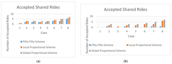
Figure 2.
A comparison of the number of acceptable rides for different schemes under (a) = 0, = 0.1 and (b) = 0, = 0.2.
Suppose = 0 and = 0.2. The numbers of acceptable rides are summarized in Table 9. According to Table 9, the numbers of acceptable rides of the Local Proportional Scheme are greater than or equal to those of the Fifty-Fifty Scheme for all test cases. These results are consistent with Theorem 1 from our previous analysis. For Case 2, Case 4, Case 5, Case 6, Case 7 and Case 8, the numbers of acceptable rides of the Global Proportional Scheme are greater than zero. Therefore, the numbers of acceptable rides of the Global Proportional Scheme are greater than or equal to those of the Fifty-Fifty Scheme according to Table 9. These results are consistent with the theoretical result of Theorem 4 in this paper. For Case 2, Case 4, Case 5, Case 6, Case 7 and Case 8, the numbers of acceptable rides of the Global Proportional Scheme are greater than zero. Therefore, the numbers of acceptable rides of the Global Proportional Scheme are greater than or equal to those of the Local Proportional Scheme according to Table 9. These results are consistent with the theoretical result of Theorem 2 in this paper.
For Case 1 and Case 3, the numbers of acceptable rides of the Global Proportional Scheme are zero. Therefore, the numbers of acceptable rides of the Global Proportional Scheme are less than or equal to those of the Fifty-Fifty Scheme according to Table 9. These results are consistent with the theoretical result of Theorem 5 developed in this paper. For Case 1 and Case 3, the numbers of acceptable rides of the Global Proportional Scheme are zero. Therefore, the numbers of acceptable rides of the Global Proportional Scheme are less than or equal to those of the Local Proportional Scheme according to Table 9. These results are consistent with the theoretical result of Theorem 3 in this paper.
To compare the performance of all test cases for = 0 and = 0.2 under the three schemes, a bar chart based on the experimental results is shown in Figure 2b. It clearly indicates that the Global Proportional Scheme either performs as well as or the same as the other two schemes for Case 2, Case 4, Case 5, Case 6, Case 7 and Case 8 (Theorem 2 and Theorem 4). The Global Proportional Scheme, however, is not better than the other two schemes for Case 1 and Case 3 (Theorem 3 and Theorem 5).
Suppose = 0.2 and = 0.1. In this case, a ride will be accepted as an acceptable shared ride only if the rewarding rates for the driver and the passenger are jointly greater than or equal to 0.1. For the results in Table 10, Table 11, Table 12 and Table 13, the numbers of acceptable rides are summarized in Table 14 for = 0.2 and = 0.1. According to Table 14, the numbers of acceptable rides under the Local Proportional Scheme are greater than or equal to those under the Fifty-Fifty Scheme for all test cases. These results are consistent with Theorem 1 from our previous analysis. The numbers of acceptable rides under the Global Proportional Scheme are greater than or equal to those under the Fifty-Fifty Scheme according to Table 14. These results are consistent with the theoretical result of Theorem 4 developed in this paper. Additionally, the numbers of acceptable rides under the Global Proportional Scheme are greater than or equal to those under the Local Proportional Scheme according to Table 14. These results are consistent with the theoretical result of Theorem 2.
Table 10.
Rewarding rate of Case 1 and Case 2 for = 0.2.
Table 11.
Rewarding rate of Case 3 and Case 4 for = 0.2.
Table 12.
Rewarding rate of Case 5 and Case 6 for = 0.2.
Table 13.
Rewarding rate of Case 7 and Case 8 for = 0.2.
Table 14.
Number of successful share rides for (a) = 0.2, = 0.1 and (b) = 0.2, = 0.2.
The numbers of acceptable rides are summarized in Table 14 for = 0.2 and = 0.2. According to Table 14, the numbers of acceptable rides under the Local Proportional Scheme are greater than or equal to those under the Fifty-Fifty Scheme for all test cases. These results are consistent with Theorem 1 from our previous analysis.
For all cases, the numbers of acceptable rides under the Global Proportional Scheme are zero. Therefore, the numbers of acceptable rides under the Global Proportional Scheme are less than or equal to those under the Fifty-Fifty Scheme according to Table 14. These results are consistent with the theoretical result of Theorem 5 in this paper. For all cases, the numbers of acceptable rides under the Global Proportional Scheme are zero. Therefore, the numbers of acceptable rides under the Global Proportional Scheme are less than or equal to those under the Local Proportional Scheme according to Table 14. These results are consistent with the theoretical result of Theorem 3 in this paper.
To compare the performance of all test cases for = 0.2 and = 0.1 under the three schemes, a bar chart based on the experimental results is shown in Figure 3b. It clearly indicates that the Global Proportional Scheme either performs as well as or the same as the other two schemes.

Figure 3.
A comparison of the number of acceptable rides for different schemes under (a) = 0.2, = 0.1 and (b) = 0.2, = 0.2.
To compare the performance of all test cases for = 0.2 and = 0.2 under the three schemes, a bar chart based on the experimental results is shown in Figure 3. It clearly indicates that the Global Proportional Scheme is either the worst among all three schemes or not better than the other two schemes as the number of acceptable rides is zero for all cases (Theorems 3 and 5).
8. Discussion
The number of acceptable shared rides is an important performance index for assessing shared mobility systems. In a shared mobility system, drivers and passengers will share rides only if they can benefit from cost savings significantly. Depending on the scheme used to allocate cost savings, the benefits of individual participants vary. Adoption of different schemes to allocate cost savings will not only influence the cost savings for drivers and passengers but also the number of acceptable shared rides, which is closely related to the number of ridesharing passengers. An important issue is to study the influence of different schemes to allocate cost savings on the number of acceptable shared rides.
Development of a decision support system for shared mobility is usually broken down into two subproblems: (a) a ridesharing optimization subproblem to match potential drivers and passengers and (b) a cost savings allocation subproblem. In the literature, although the ridesharing optimization problem has been studied extensively and there are many schemes to allocate cost savings in ridesharing systems, the effectiveness of different schemes to allocate cost savings is less explored. In practice, simple rules have been used to solve the cost savings allocation problem based on proportional methods [11,12,13] to reduce computational complexity. Improper allocation of cost savings may lead to dissatisfaction of drivers and passengers and reduce the number of shared rides that can be accepted by the drivers and passengers. However, effectiveness of these proportional cost savings allocation schemes in a shared mobility system needs to be studied. The influence of applying different schemes to allocate cost savings on the number of acceptable shared rides is an important issue in the design of shared mobility systems.
In this study, we explore effectiveness of the three different proportional schemes proposed in [11,12,13] by theoretical analysis. Shared rides recommended by shared mobility systems are typically optimized for objective functions such as overall travel distance. Therefore, not all recommended shared rides are satisfactory or acceptable for drivers and passengers. The analysis in this paper characterizes several properties and conditions under which one proportional cost savings allocation scheme outperform another in terms of the number of rides acceptable by the drivers and passengers. These properties provide a foundation for selecting the proper proportional scheme to allocate cost savings. These properties are supported by experimental results of several test cases provided in this paper. Our theoretical analysis and properties are consistent with the experimental results. Although our analysis indicates that, among the three schemes analyzed in this study, none always dominates the other two under any situation, but a dominating property does exist under a specific situation. These properties provide the information about the influence of cost savings allocation schemes on the number of acceptable shared rides. If the minimal expected rewarding rate can be satisfied under the Global Proportional Scheme, then the Global Proportional Scheme is the best scheme among the three schemes studied in this paper. Otherwise, the Local Proportional Scheme is the best scheme among the three schemes. The Fifty-Fifty Scheme should not be used due to its poor performance.
The properties and results presented in this study are based on the assumption that drivers and passengers will not accept ridesharing in case the minimal expected rewarding rate cannot be attained. Several studies [31,32] indicate that cost savings are one important factor for ridesharing. Therefore, the results of these studies justify this assumption of this paper. The theory presented in this study does not hinge on the assumption that “travel cost is proportional to distance”, which is used in [11,12]. The decision model adopted in this study consists of a practical general framework and procedures that consider spatial, time, capacity and detour ratio [13], and can consider even social factors [22]. The discussions above indicate that theory developed in this study is based on a problem setting in actual practice and also illustrate the validity and practicality of the theory developed in this study.
The results of this study generate interesting and important research questions: Do any other rules exist that are similar or dissimilar to the ones uncovered in this paper among other cost allocation schemes? Do any other rules exist among other cost allocation schemes and the three schemes studied in this paper? These open problems call for further studies.
9. Conclusions
Shared mobility is a transportation mode motivated by sharing vehicles to reduce the cost of journey, fuel consumption, emissions and air pollution. As cost savings are the primary incentive for the shared mobility mode, most studies on shared mobility focus on optimization of the travel distance to reduce cost. Due to computational complexity, the issue to allocate cost savings among stakeholders is often done by applying proportional methods such as the Fifty-Fifty Scheme, Local Proportional Scheme and Global Proportional Scheme, which are easy to implement in shared mobility systems. However, effectiveness of these proportional methods has not been analyzed and compared in the literature. In addition, there is no guideline on how to select the proper proportional method to allocate cost savings and how different proportional methods to allocate cost savings influence performance or acceptance of shared rides. This study provides a theoretical study on comparison of three different proportional methods in the literature for allocation of cost savings. Our study is based on the fact that potential drivers and passengers may reject the shared rides recommended by the shared mobility system if the rewarding rates are lower than their expectations. As the proportional method used to allocate cost savings among drivers and passengers directly influences the rewarding rates, the number of acceptable rides will be influenced by the method used to allocate cost savings. Therefore, we focus on comparing the number of acceptable rides under given minimal expected rewarding rate of the potential drivers and passengers. Through our analysis, we find several useful properties that can serve as a guideline for selecting a proper method from the Fifty-Fifty Scheme, Local Proportional Scheme and Global Proportional Scheme. These properties indicate that if the rewarding rate under the Global Proportional Scheme is greater than or equal to minimal expected rewarding rate, the Global Proportional Scheme is the best among the three proportional methods. Otherwise, the Fifty-Fifty Scheme and Local Proportional Scheme will be better than the Global Proportional Scheme. The properties established in this study also indicate that the Local Proportional Scheme is better or no worse than the Fifty-Fifty Scheme. These properties provide insights into which proportional method should be used to achieve more acceptable shared rides. Although the three schemes studied in this paper are often adopted in industry and academia, practitioners and researchers using these three schemes in ridesharing systems are not aware of their influence on acceptance of shared rides. The results of this study uncover some useful rules for selecting the three schemes to allocate cost savings. These results can be applied by policy makers and service providers to use the correct scheme to achieve more acceptable shared rides by following the rules: (1) the Fifty-Fifty Scheme should not be used, (2) choose the Global Proportional Scheme if the rewarding rate under the Global Proportional Scheme is greater than or equal to the minimal expected rewarding rate and (3) choose the Local Proportional Scheme if the rewarding rate under the Global Proportional Scheme is less the minimal expected rewarding rate. These rules can be easily implemented. An interesting future research direction will be to study and analyze effectiveness of other methods used for allocation of cost savings in the context of shared mobility systems to discover other useful rules to achieve more acceptable shared rides. Results call for further studies in this interesting and challenging research direction.
Funding
This research was supported in part by the Ministry of Science and Technology, Taiwan, under Grant MOST 110-2410-H-324-001.
Institutional Review Board Statement
Not applicable.
Informed Consent Statement
Not applicable.
Data Availability Statement
Data available in a publicly accessible repository described in the article.
Acknowledgments
The author would like to thank the anonymous reviewers and the editors for their comments and suggestions, which are invaluable for the author to improve presentation, clarity and quality of this paper.
Conflicts of Interest
The author declares no conflict of interest.
Appendix A
Proof of Lemma 3.
To show the minimal rewarding rate for passengers under the Local Proportional Scheme is less than or equal to that of the Global Proportional Scheme, we must show that
Let be the winning bid of driver such that .
Note that .
As ,
Note that
Hence .
Therefore, the minimal rewarding rate for passengers under Local Proportional Scheme is less than or equal to that of Global Proportional Scheme. □
Appendix B
Proof of Lemma 4.
We first show that the minimal rewarding rate for drivers under the Local Proportional Scheme is less than that of the Global Proportional Scheme. To show the minimal rewarding rate for drivers under the Local Proportional Scheme is less than or equal to that of the Global Proportional Scheme, we must show that
Let be the winning bid of driver such that .
It follows that .
As ,
Note that
Therefore the minimal rewarding rate for drivers under the Local Proportional Scheme is less than or equal to that of the Global Proportional Scheme. □
Appendix C
Proof of Lemma 5.
Let be the ride corresponding to the winning bid of driver such that .
To show the maximal rewarding rate for passengers under the Local Proportional Scheme is greater than or equal to that of the Global Proportional Scheme, we must show that .
Note that
As ,
Note that
Therefore the maximal rewarding rate for passengers under the Local Proportional Scheme is greater than or equal to that of the Global Proportional Scheme.
As the rewarding rate for driver is and , the maximal rewarding rate for the drivers under the Local Proportional Scheme is greater than or equal to that of the Global Proportional Scheme. □
References
- The International Energy Agency (IEA). Tracking Report. Available online: https://www.iea.org/reports/tracking-transport-2020 (accessed on 20 August 2021).
- Hossain, M. Sharing economy: A comprehensive literature review. Int. J. Hosp. Manag. 2020, 87, 102470. [Google Scholar] [CrossRef]
- Klarin, A.; Suseno, Y. A state-of-the-art review of the sharing economy: Scientometric mapping of the scholarship. J. Bus. Res. 2021, 126, 250–262. [Google Scholar] [CrossRef]
- Hyland, M.; Mahmassani, H.S. Operational benefits and challenges of shared-ride automated mobility-on-demand services. Transp. Res. Part A: Policy Pr. 2020, 134, 251–270. [Google Scholar] [CrossRef]
- Furuhata, M.; Dessouky, M.; Ordóñez, F.; Brunet, M.; Wang, X.; Koenig, S. Ridesharing: The state-of-the-art and future direc-tions. Transp. Res. Pt. B-Methodol. 2013, 57, 28–46. [Google Scholar] [CrossRef]
- Agatz, N.; Erera, A.; Savelsbergh, M.; Wang, X. Optimization for dynamic ride-sharing: A review. Eur. J. Oper. Res. 2012, 223, 295–303. [Google Scholar] [CrossRef]
- Mourad, A.; Puchinger, J.; Chu, C. A survey of models and algorithms for optimizing shared mobility. Transp. Res. Part B: Methodol. 2019, 123, 323–346. [Google Scholar] [CrossRef]
- Martins, L.D.C.; de la Torre, R.; Corlu, C.G.; Juan, A.A.; Masmoudi, M.A. Optimizing ride-sharing operations in smart sustainable cities: Challenges and the need for agile algorithms. Comput. Ind. Eng. 2021, 153, 107080. [Google Scholar] [CrossRef]
- Santos, D.O.; Xavier, E.C. Taxi and Ride Sharing: A Dynamic Dial-a-Ride Problem with Money as an Incentive. Expert Syst. Appl. 2015, 42, 6728–6737. [Google Scholar] [CrossRef]
- Guajardoa, M.; Ronnqvist, M. A review on cost allocation methods in collaborative transportation. Int. Trans. Oper. Res. 2016, 23, 371–392. [Google Scholar] [CrossRef]
- Wang, X.; Agatz, N.; Erera, A. Stable Matching for Dynamic Ride-Sharing Systems. Transp. Sci. 2018, 52, 850–867. [Google Scholar] [CrossRef]
- Agatz, N.A.H.; Erera, A.L.; Savelsbergh, M.W.P.; Wang, X. Dynamic ride-sharing: A simulation study in metro Atlanta. Transp. Res. Part B: Methodol. 2011, 45, 1450–1464. [Google Scholar] [CrossRef]
- Hsieh, F.-S.; Zhan, F.-M.; Guo, Y.-H. A solution methodology for carpooling systems based on double auctions and cooperative coevolutionary particle swarms. Appl. Intell. 2018, 49, 741–763. [Google Scholar] [CrossRef]
- Jin, S.T.; Kong, H.; Wu, R.; Sui, D.Z. Ridesourcing, the sharing economy, and the future of cities. Cities 2018, 76, 96–104. [Google Scholar] [CrossRef]
- Shaheen, S.; Chan, N. Mobility and the sharing economy: Potential to facilitate the first- and last-mile public transit connec-tions. Built Environ. 2016, 42, 573–588. [Google Scholar] [CrossRef]
- Lokhandwala, M.; Cai, H. Dynamic ride sharing using traditional taxis and shared autonomous taxis: A case study of NYC. Transp. Res. Part C: Emerg. Technol. 2018, 97, 45–60. [Google Scholar] [CrossRef]
- Li, R.; Liu, Z.; Zhang, R. Studying the benefits of carpooling in an urban area using automatic vehicle identification data. Transp. Res. Part C: Emerg. Technol. 2018, 93, 367–380. [Google Scholar] [CrossRef]
- Baldacci, R.; Maniezzo, V.; Mingozzi, A. An exact method for the car pooling problem based on Lagrangean column genera-tion. Oper. Res. 2004, 52, 422–439. [Google Scholar] [CrossRef]
- Kaan, L.; Olinick, E.V. The Vanpool Assignment Problem: Optimization models and solution algorithms. Comput. Ind. Eng. 2013, 66, 24–40. [Google Scholar] [CrossRef]
- Li, B.; Krushinsky, D.; Reijers, H.A.; Van Woensel, T. The Share-a-Ride Problem: People and parcels sharing taxis. Eur. J. Oper. Res. 2014, 238, 31–40. [Google Scholar] [CrossRef] [Green Version]
- Masson, R.; Trentini, A.; Lehuédé, F.; Malhéné, N.; Péton, O.; Tlahig, H. Optimization of a city logistics transportation system with mixed passengers and goods. EURO J. Transp. Logist. 2017, 6, 81–109. [Google Scholar] [CrossRef] [Green Version]
- Hsieh, F.-S. A Particle Swarm Optimization Algorithm to Meet Trust Requirements in Ridesharing Systems. In Proceedings of the 2020 11th IEEE Annual Ubiquitous Computing, Electronics & Mobile Communication Conference (UEMCON), New York, NY, USA, 28–31 October 2020; pp. 592–595. [Google Scholar]
- Narayanan, S.; Chaniotakis, E.; Antoniou, C. Shared autonomous vehicle services: A comprehensive review. Transp. Res. Part C: Emerg. Technol. 2020, 111, 255–293. [Google Scholar] [CrossRef]
- Hosni, H.; Naoum-Sawaya, J.; Artail, H. The shared-taxi problem: Formulation and solution methods. Transp. Res. Part B: Methodol. 2014, 70, 303–318. [Google Scholar] [CrossRef]
- Schreieck, M.; Safetli, H.; Siddiqui, S.A.; Pflügler, C.; Wiesche, M.; Krcmar, H. A matching algorithm for dynamic rideshar-ing. Transp. Res. Procedia 2016, 19, 272–285. [Google Scholar] [CrossRef]
- Cheikh-Graiet, S.B.; Dotoli, M.; Hammadi, S. A Tabu Search based metaheuristic for dynamic carpooling optimization. Comput. Ind. Eng. 2020, 140, 106217. [Google Scholar] [CrossRef]
- Hsieh, F.S. A Comparative Study of Several Metaheuristic Algorithms to Optimize Monetary Incentive in Ridesharing Sys-tems. ISPRS Int. J. Geo-Inf. 2020, 9, 590. [Google Scholar] [CrossRef]
- Hsieh, F.-S. Ridesharing based on a Discrete Self-adaptive Differential Evolution Algorithm. In Proceedings of the 2020 11th IEEE Annual Information Technology, Electronics and Mobile Communication Conference (IEMCON), Vancouver, BC, Canada, 4–7 November 2020; pp. 696–700. [Google Scholar]
- Jung, J.; Jayakrishnan, R.; Park, J.Y. Dynamic Shared-Taxi Dispatch Algorithm with Hybrid-Simulated Annealing. Comput. Civ. Infrastruct. Eng. 2016, 31, 275–291. [Google Scholar] [CrossRef]
- Butler, L.; Yigitcanlar, T.; Paz, A. Barriers and risks of Mobility-as-a-Service (MaaS) adoption in cities: A systematic review of the literature. Cities 2021, 109, 103036. [Google Scholar] [CrossRef]
- Van Der Waerden, P.; Lem, A.; Schaefer, W. Investigation of Factors that Stimulate Car Drivers to Change from Car to Carpooling in City Center Oriented Work Trips. Transp. Res. Procedia 2015, 10, 335–344. [Google Scholar] [CrossRef] [Green Version]
- Shaheen, S.A.; Chan, N.D.; Gaynor, T. Casual carpooling in the San Francisco Bay Area: Understanding user characteristics, behaviors, and motivations. Transp. Policy 2016, 51, 165–173. [Google Scholar] [CrossRef] [Green Version]
- Shapley, L.S. A Value for N-Person Games. A Value N-Person Games 1952, 28, 307–317. [Google Scholar] [CrossRef]
- Schmeidler, D. The Nucleolus of a Characteristic Function Game. SIAM J. Appl. Math. 1969, 17, 1163–1170. [Google Scholar] [CrossRef]
- Kalai, E. Proportional solutions to bargaining situations: Intertemporal utility comparisons. Econometrica 1977, 45, 1623–1630. [Google Scholar] [CrossRef]
- Fatima, S.S.; Wooldridge, M.; Jennings, N.R. A linear approximation method for the Shapley value. Artif. Intell. 2008, 172, 1673–1699. [Google Scholar] [CrossRef] [Green Version]
- Perea, F.; Puerto, J. A heuristic procedure for computing the nucleolus. Comput. Oper. Res. 2019, 112, 104764. [Google Scholar] [CrossRef]
- Berger, S.; Bierwirth, C. Solutions to the request reassignment problem in collaborative carrier networks. Transp. Res. Part E: Logist. Transp. Rev. 2010, 46, 627–638. [Google Scholar] [CrossRef]
- Özener, O. Örsan Developing a Collaborative Planning Framework for Sustainable Transportation. Math. Probl. Eng. 2014, 2014, 1–14. [Google Scholar] [CrossRef]
- Flisberg, P.; Frisk, M.; Röonnqvist, M.; Guajardo, M. Potential savings and cost allocations for forest fuel transportation in Sweden: A country-wide study. Energy 2015, 85, 353–365. [Google Scholar] [CrossRef]
- Lu, W.; Quadrifoglio, L. Fair cost allocation for ridesharing services – modeling, mathematical programming and an algorithm to find the nucleolus. Transp. Res. Part B: Methodol. 2019, 121, 41–55. [Google Scholar] [CrossRef] [Green Version]
- Zhang, C.; Xie, J.; Wu, F.; Gao, X.; Chen, G. Pricing and allocation algorithm designs in dynamic ridesharing system. Theor. Comput. Sci. 2020, 803, 94–104. [Google Scholar] [CrossRef]
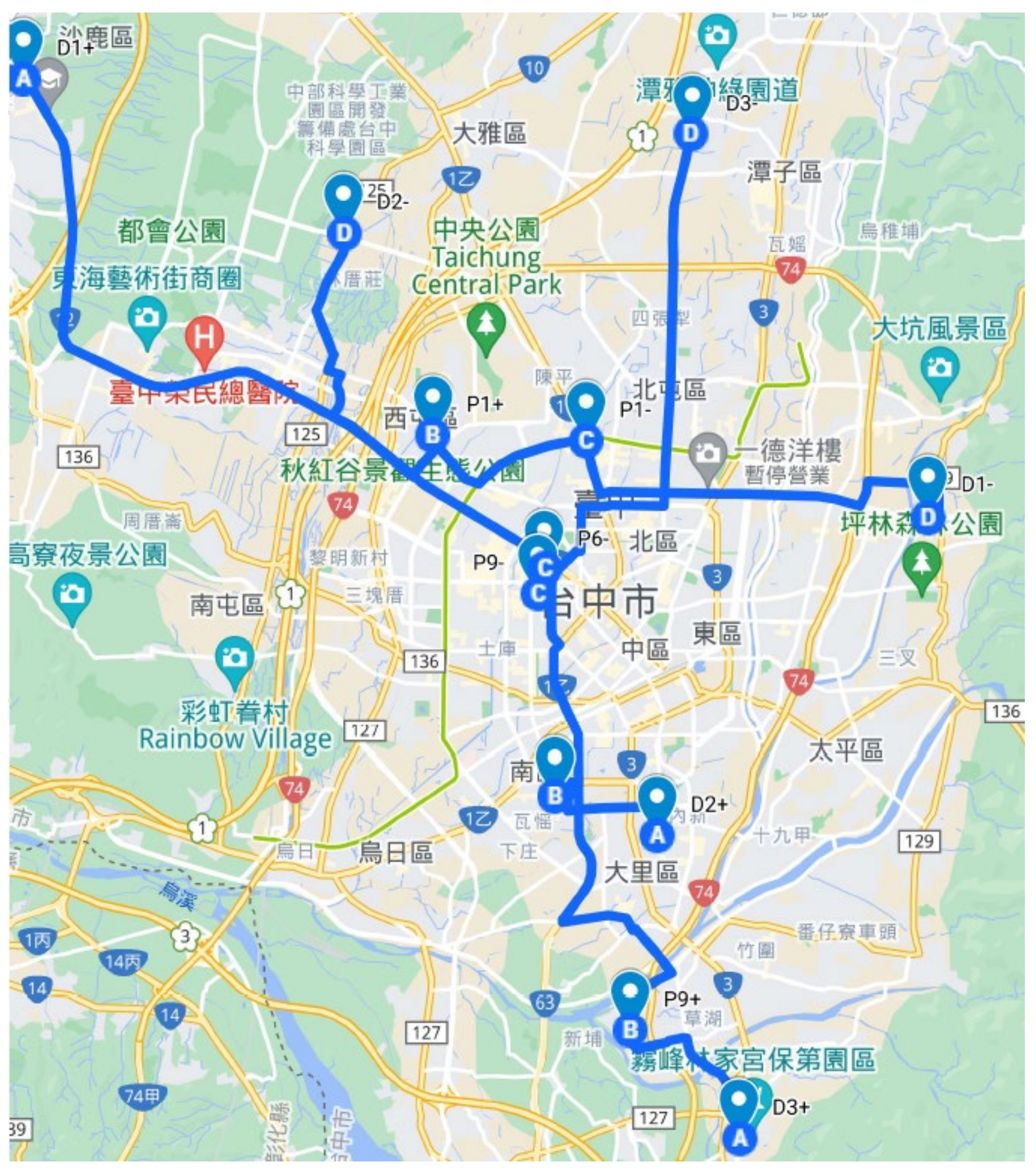
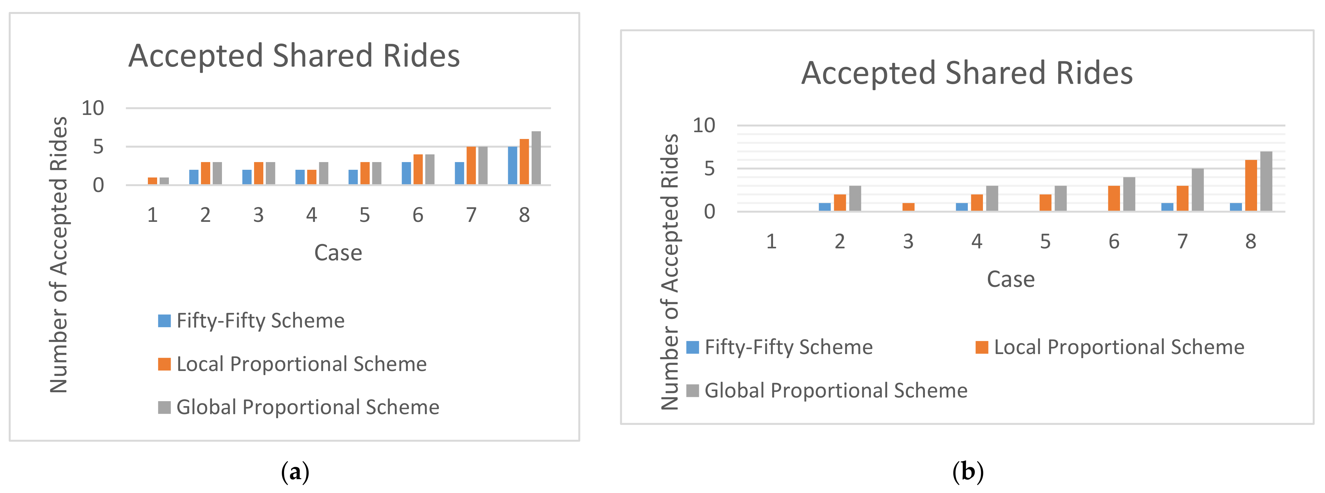
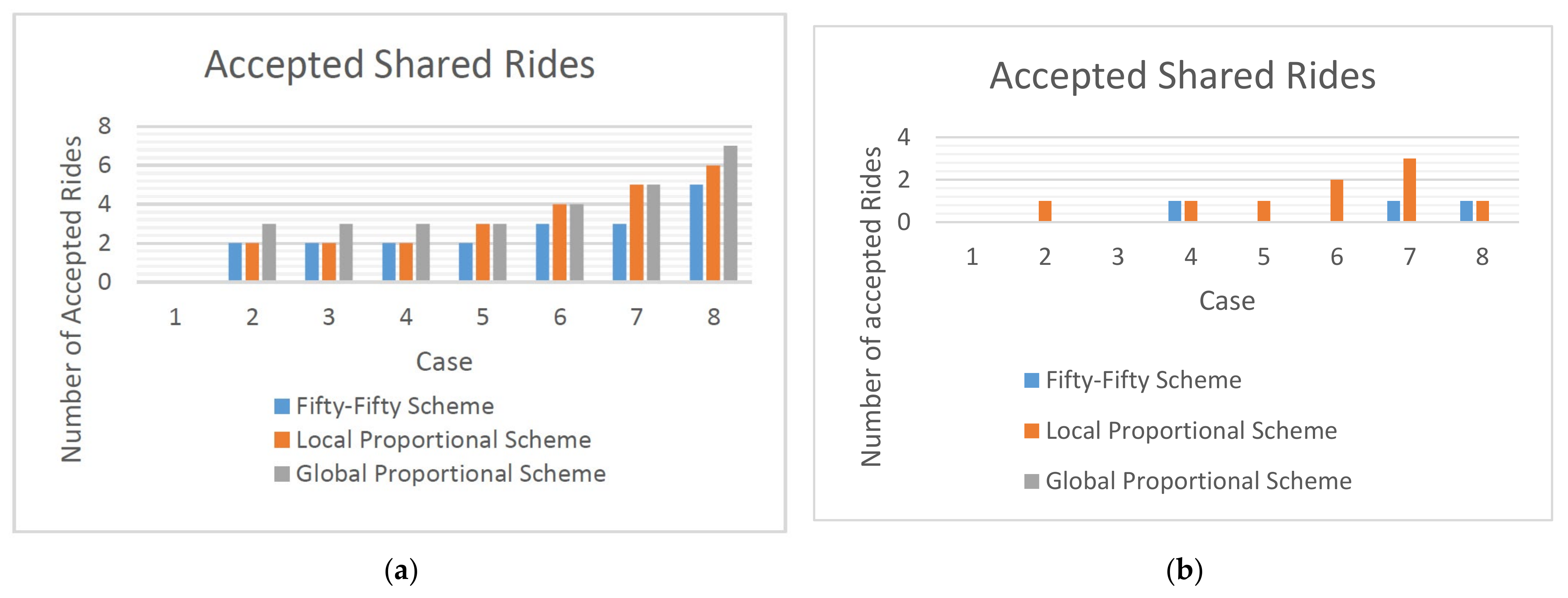
Publisher’s Note: MDPI stays neutral with regard to jurisdictional claims in published maps and institutional affiliations. |
© 2021 by the author. Licensee MDPI, Basel, Switzerland. This article is an open access article distributed under the terms and conditions of the Creative Commons Attribution (CC BY) license (https://creativecommons.org/licenses/by/4.0/).