Abstract
Roughness is an important factor affecting the engineering stability of jointed rock masses. The existing roughness evaluation methods are all based on a uniform sampling interval, which changes the geometrical morphology of the original profile and inevitably ignores the influence of secondary fluctuations on the roughness. Based on the point cloud data obtained by 3D laser scanning, a non-equal interval sampling method and an equation for determining the sampling frequency on the roughness profile are proposed. The results show that the non-equal interval sampling method can successfully maintain the morphological characteristics of the original profile and reduce the data processing cost. Additionally, direct shear tests under constant normal load (CNL) conditions are carried out to study the influence of roughness anisotropy on the shear failure mechanism of joint surfaces. It is found that with the increase in shear displacement, the variations in the shear stress are related to the failure mechanisms of dilatancy and shear fracture of the joint. Finally, the distributions of shear stress, dilatancy and fracture areas on the rough joint in different shear directions are calculated theoretically. Results show that the anisotropy and failure mechanism of rough joint can be well characterized by the modified root mean square parameter Z2′.
1. Introduction
The safety and stability of jointed rock masses are mainly controlled by the mechanical behavior of the joints. Many factors, such as the mineral composition, geometrical morphology, roughness and fillers, will significantly affect the mechanical characteristics of the jointed rock mass. Thus, a coupled thermal-hydrological-mechanical model is employed to investigate the permeability evolution and fault reactivation of a critically stressed fault in geothermal reservoir [1]. The Mohr–Coulomb model is commonly used in practice to evaluate the mechanical properties of geotechnical materials [2]. Roughness will affect the apparent cohesion and friction angle, changing the dilatancy and the peak shear strength of rock joints [3]. This means that the roughness of the joint surface is a critical factor in determining the shear strength of rock joints [4]. Consequently, reasonable characterization of the joint surface roughness and establishment of the correlation between roughness parameters and shear strength are helpful to evaluate the mechanical behavior of rock joints.
Initially, 10 standard profiles are used to visually and qualitatively evaluate rock joint roughness [5]. By comparing the surface morphology of natural joints with the standard profiles, the most similar profile is selected. The corresponding JRC value can be easily and quickly obtained by the empirical comparison method, although this is strongly dependent on the experience of the engineer. Thus, scholars pay more attention to the quantitative description of roughness. Many roughness characterization methods, such as fractal [6], structure functions (SF) [7] and power spectral density (PSD) [8], have been established. Recently, Ünlüsoy and Süzen [9] proposed a new method for automatically estimating the JRC of a 2D profile based on PSD. Aslam [10] presented a new approach to determining roughness coefficient neutrosophic numbers using the neutrosophic exponentially weighted moving average, which is convenient to apply without fitting the functions. The root mean square of the first deviation of the profile Z2 has become a widely used roughness evaluation parameter, although Z2 only considers the effect of the local inclination angle and ignores the influence of the overall amplitude of the profiles on the roughness. Zhang et al. [3] introduced a new roughness index (λ) based on Z2, which considers the inclination angle, amplitude of asperities and their directions. Magsipoc et al. [11] conducted a comprehensive review of commonly used 2D and 3D surface roughness characterization methods. They suggested that 2D profiles may obscure or exaggerate the roughness features, and 3D roughness characterization methods should be considered for the development of surface measurement technology. A digital image processing (DIP) technique was used to reconstruct the surface morphology of joints [12], and a variogram function was adopted to characterize the anisotropy of the joint surface roughness and estimate the joint aperture. Moreover, the effects of the sampling interval and anisotropy on roughness parameters SF, Z2 and Rp were studied utilizing point cloud data obtained by 3D laser scanning [13]. By averaging the equivalent height difference in the shear direction to reflect the fluctuation and directivity of the joint surface morphology, Ban et al. [14] proposed a new roughness parameter called the average equivalent height difference (AHD), while the fractal dimension of AHD was used to characterize the scale effect of roughness. The effects of joint surface roughness and anisotropy on the size and shape of the excavation damage zone in jointed rocks were examined by numerical simulation [15]. Using a class ratio transform method, the geometric irregularities of the roughness parameters in the polar coordinate could be transformed to a regular roughness asperity pattern [16], which could be easily approximated by the ellipse function. However, the actual roughness in different directions may be ignored after smoothing processing.
The existing statistical methods for roughness evaluation significantly depend on the sampling interval (Δx) [17]. Azinfar et al. [18] studied the influences of scale effect on 3D roughness parameters such as the fractal parameter (D), amplitude parameter (A), roughness parameter (Rs) and (2A0θ*max/(C + 1)). It is noted that the sampling interval has a negative exponential relationship with the JRC value [19]. While the roughness of the joint surface AHD proposed by Ban et al. [20] has a positive size effect, there was a negative size effect and no size effect in a certain direction. The sampling interval has little influence when using volume and amplitude parameters (Van, Zsa, Zrms, and Zrange) for JRC estimation, while it has some influence when other parameters (θs, θg, θ2s, SsT and SsF) are used [21]. Thus, equations with amplitude parameters are recommended to facilitate the rapid estimation of JRC in engineering practice for their easy calculation. Huang et al. [22] analyzed the variation in fitting parameters at different values of Δx based on the relationship between JRC and statistical parameter Z2, and they established empirical formulas for JRC, Z2 and Δx. Due to the scale dependency of roughness, a changing scale will indirectly affect the surface contact mechanics, such as shear strength and dilation. Consequently, determining the optimal sampling interval is very important for accurately estimating the actual roughness and reducing the cost of data processing. Du et al. [23] proposed the concept of the effective length of the JRC scale effect and established a graphical method to identify the effective length of the JRC scale effect. Through a Fourier series reconstructed roughness profile [24], the maximum sampling interval is assigned as SImax = L/3n, where n is the order of the Fourier series and L is the length of the profile. A small sample size is generally used during roughness measurement in the laboratory, while the size of natural joint surfaces may be several meters or even longer. Yong et al. [25] developed a method for measuring the JRC values of large joints in the field. In order to overcome the deficiencies of existing approaches, Huan et al. [26] proposed a new JRC estimation method based on the back-calculation of shear strength.
Based on the point cloud data obtained by 3D laser scanning, factors that affect the roughness evaluation, such as the noise of original data and the non-stationary nature of joints, are discussed in this paper. Four roughness parameters, the roughness ratio Rp, the angle standard deviation σi, the root mean square method Z2 and the modified root mean square Z2′, are used to analyze the scale effect and anisotropy of roughness. Moreover, the reasons for the scale effect of joint surface roughness are discussed. To compensate for the deficiencies of the regular interval sampling method that changes the geometrical morphology of the original profile, a non-equal interval sampling method and an equation for determining the sampling frequency on the roughness profile are proposed. Additionally, the influence of roughness anisotropy on the shear mechanism of the joint is further discussed. The distributions of shear stress and ranges of dilatancy and non-dilatancy on the joint with different shear directions are calculated based on the direct shear test. The results are helpful for understanding the influences of the roughness sampling interval and anisotropy on the shear failure mechanism of the rock joint surface.
2. Materials and Methods
2.1. Collection of Rock Joint Specimen Point Clouds
The joint samples used in this study were collected from the construction site of Mengxi Road, which is located in Huaxi District, Guiyang City, Guizhou Province. The lithology of the joints is red argillaceous sandstone. There are three groups of joints developing in the rock mass, among which the attitude of the dominant joint is 85° ∠ 47°. In total, 20 jointed rock samples with a size of 140 mm × 140 mm × 70 mm in the x, y and z axes were collected based on the main joint. A 3D laser scanner was used to obtain the initial point cloud information of the joint surfaces’ morphology. The resolution of the scanner was 0.02 mm, and the measurement distance to the samples was controlled at around 750 mm. In order to collect specimen point clouds without losing data, multiple separate scan measurements were performed from different angles. The point cloud data obtained by multiple scans were converted into the original data in a unified coordinate system according to the relative geometric position of the joint surfaces. Geomagic Studio was used to extract the three-dimensional scanned information of the research area, and to perform noise reduction processing on the initial point cloud data. Finally, Surfer was applied to display the three-dimensional spatial information of the joint surfaces, and to obtain profiles in different directions for roughness calculation.
2.2. Direct Shear Tests
The 20 scanned contact specimens were subjected to direct shear tests considered to be under constant normal loading (CNL) conditions. However, slight variations in the normal stress can occur during the shear test owing to the tolerance of the experimental device [27]. The shear test device was composed of two blocks: a fixed inferior block and a superior block, which could move horizontally and vertically through sliding over the inferior block. A normal force F, corresponding to a normal pressure σn, was applied on top of the mobile block before the shear tests. This force F generates a normal stress σn = F/As, where As denotes the area of the horizontal section of the contact specimen. Then, the superior block was displaced horizontally by applying a horizontal force, thereby shearing the sample. Displacement sensors were used to record the horizontal and vertical displacement during the test. The accuracy of the displacement sensor was 0.01 mm. A YY-8 Type geotechnical mechanics data acquisition instrument was applied to acquire the experimental data, such as normal stress, shear stress and shear displacement, and the data collection interval was 10 ms.
3. Influence of Non-Stationary Joint on Roughness
3.1. Reasons for Non-Stationary Point Clouds
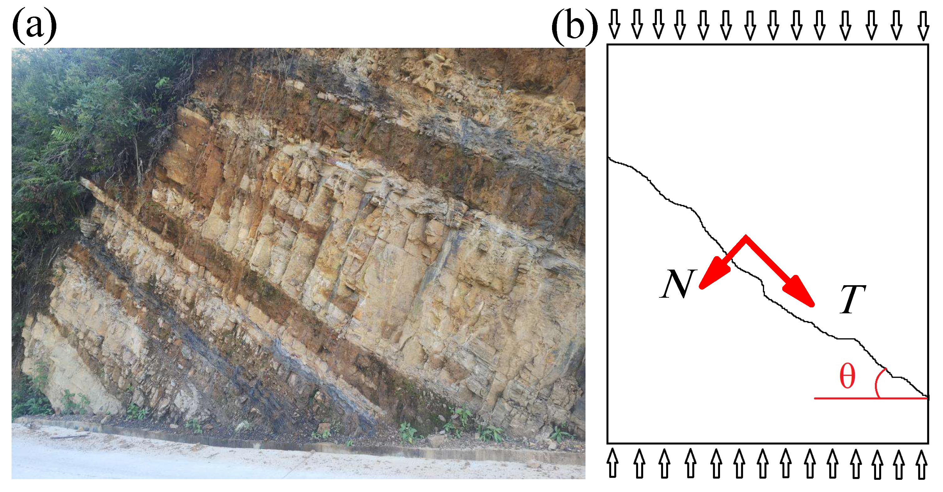
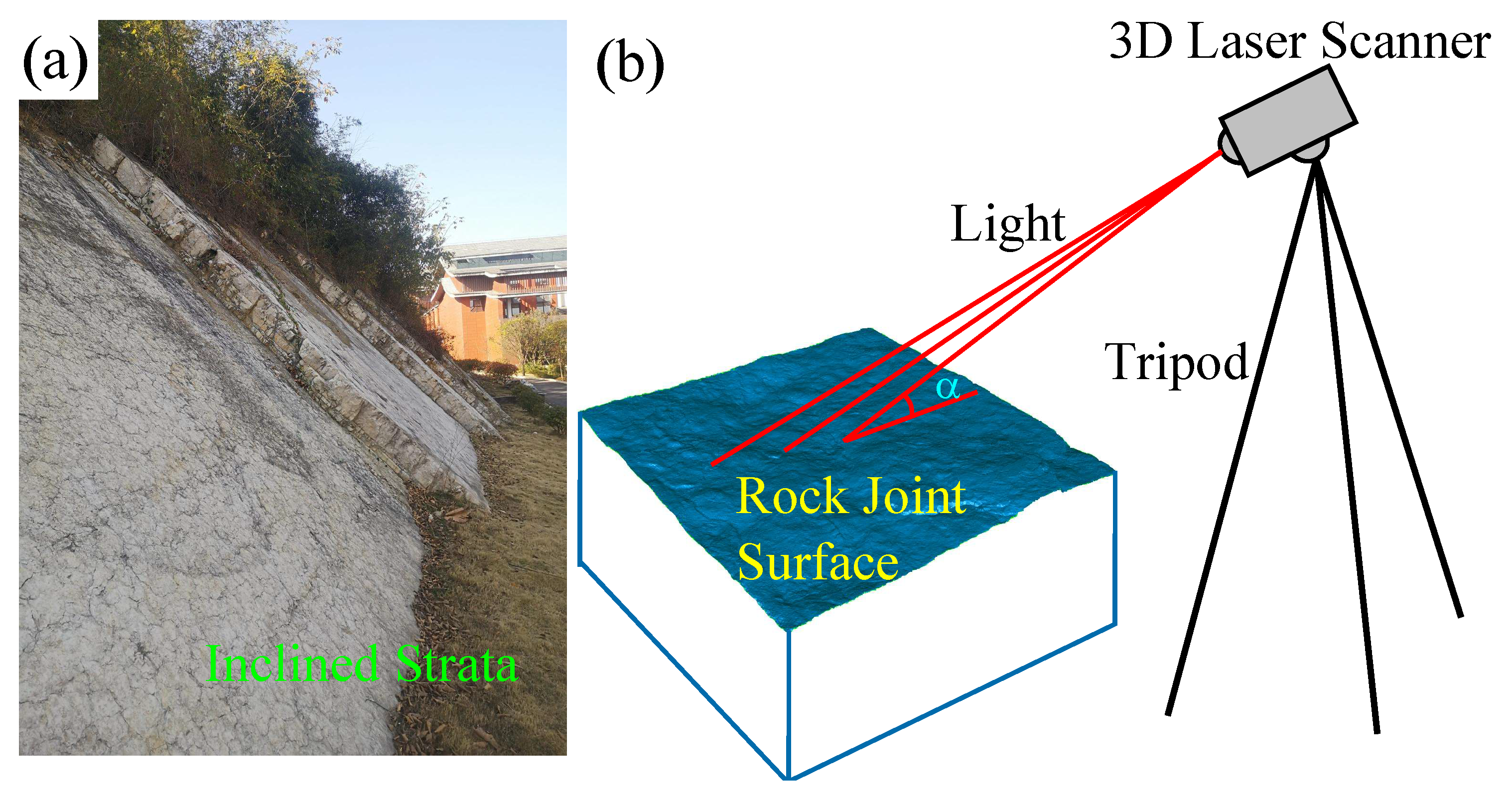
Natural rock masses are subjected to complex tectonization during their geological history, and their stratification is generally present at a certain angle in the horizontal direction (Figure 1a). The inclination direction of the joint surface usually becomes the dominant direction for failure under stress (Figure 1b). The inclination of the joint surface (Figure 2a) and the non-perpendicular application of light from a 3D laser scanner to the joint surface (Figure 2b) will cause the point cloud data obtained to be non-stationary. However, the estimation of joint surface roughness requires the point cloud to be referenced to the horizontal plane. Ge et al. [28] found that the inclination of the joint surface has an important influence on the roughness calculation, and a method of transforming the spatial coordinate system was used to eliminate the influence of joint surface inclination. Bitenc et al. [29] established an optimal wavelet-denoising procedure for terrestrial laser scanning data acquired with different scanning ranges and incidence angles, and rock discontinuities having different roughness characteristics and surface reflectivity.

Figure 1.
Joint surfaces in rock mass. (a) Inclined state of natural rock; (b) Schematic diagram of forces exerted on joint surface.
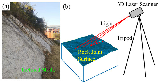
Figure 2.
Reasons for non-stationary point clouds. (a) Joint surface with an inclination angle; (b) Non-perpendicular application of light from a 3D laser scanner to the joint surface.
3.2. Removing the Non-Stationary Feature of Point Clouds
Assume that P(x0, y0, z0) is a source point cloud with non-stationary features and that Q(x, y, z) is the target point cloud without non-stationary features. The following steps are required for removing the influence of non-stationarity.
Capturing the original point clouds of rock joints by a 3D laser scanner.
Denoising the original point clouds.
Creating the grid data: the original point clouds are converted into grid data using the minimum curvature interpolation method (Figure 3a).
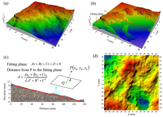
Figure 3.
Method for removing the inclination features of rock joints. (a) Grid data processed by denoising and minimum curvature interpolation; (b) Fitting plane; (c) Calculating the distance from original point cloud to the fitting plane; (d) Joint without inclined features.
Fitting a plane to the points: the least squares multiple linear regression method is adopted to obtain the best fitting plane equation of the point cloud of rock joints, which is Ax + By + Cz + D = 0 (Figure 3b).
Calculating the distance from point P(x0, y0, z0) in the grid data to the fitting plane (Figure 3c).
Removing the non-stationary features: new point clouds are generated, taking the X and Y coordinates of the point P(x0, y0, z0) as the X and Y coordinates of the target point, and letting the calculated distance d be the Z coordinate of the target point, namely Q(x0, y0, d) (Figure 3d).
4. Estimation of Joint Surface Roughness
4.1. Methods Used to Evaluate JRC
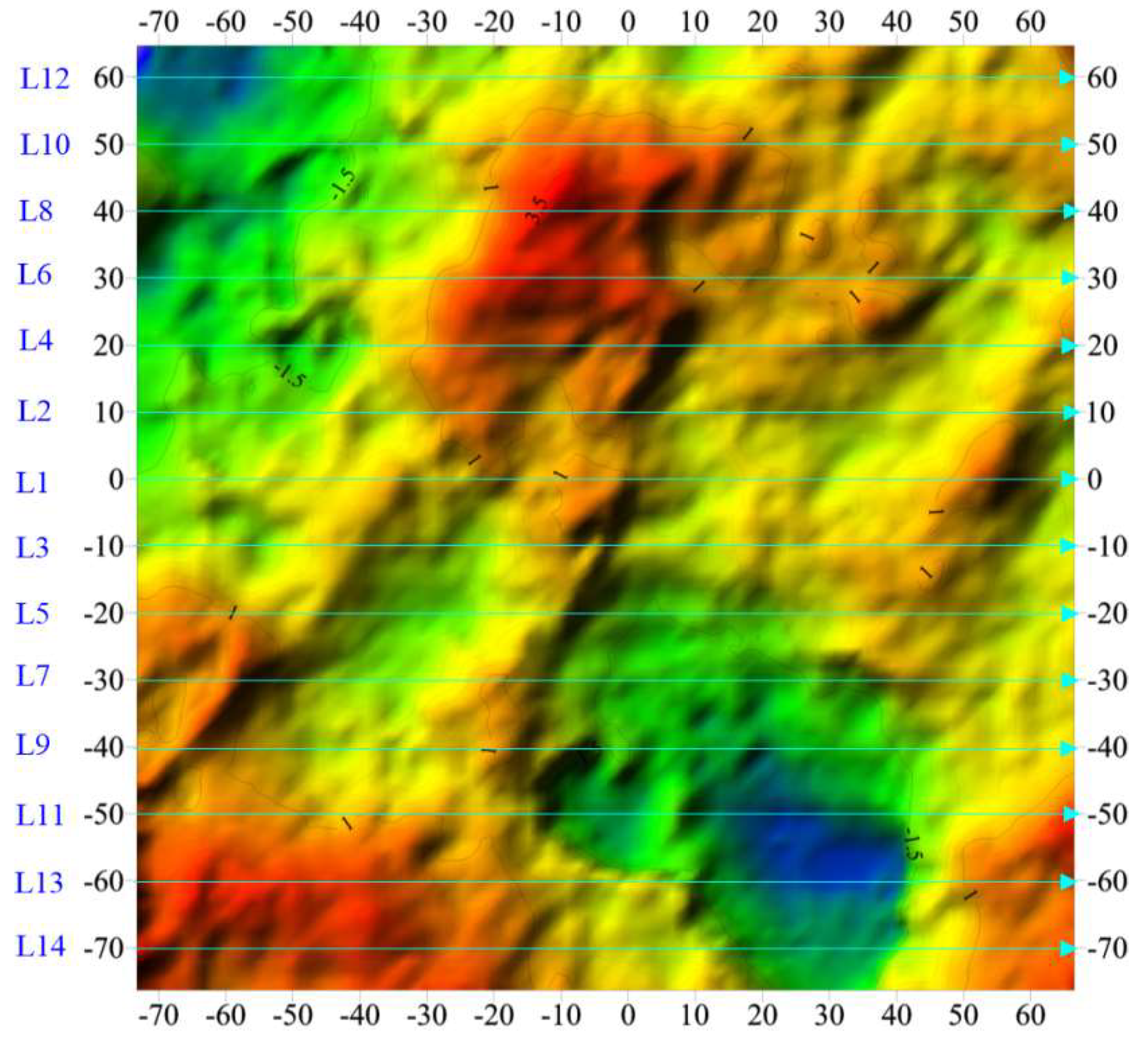
Numerous methods to represent joint surface roughness have been proposed previously [11]. Li and Zhang [30] systematically studied the 15 parameters and 47 empirical equations that are used to evaluate JRC. They found that in terms of correlation coefficients, the angle standard deviation σi and the root mean square of the first deviation of the profile Z2 are the best. In this paper, 14 parallel profile lines along the shear direction with an interval of 10 mm were intercepted from the study region after the pretreatment process of original point clouds obtained by a 3D laser scanner (Figure 4). Digitized information about the intercepted lines was extracted, and the coordinate values for each point on the lines were obtained. The roughness ratio Rp, σi, Z2 and modified Z2′ were taken to estimate the roughness of each profile. Finally, the average roughness of each profile was adopted to characterize the roughness of the joint surface.
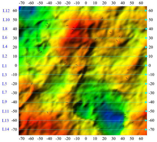
Figure 4.
Fourteen parallel profile lines along the shear direction.
Roughness ratio Rp
The roughness ratio Rp is the ratio of the actual length of a profile to the nominal length of the profile [31]:
where L is the length of the profile; xi and yi are points along the profile of the x and y coordinates, respectively.
Standard deviation of the angle σi
The standard deviation of local angle i on the profile line is defined as [32]:
Root Mean Square method Z2
Amplitude parameters cannot account for local fluctuations and sloping of the profile; these local fluctuations and sloping of the profile play an important role in the mechanical behavior of the joints. Myers [33] proposed a parameter to estimate the roughness with the root mean square of the average local slope Z2, which has become one of the most commonly used parameters.
where Z2 is the root mean square of the first deviation of the profile.
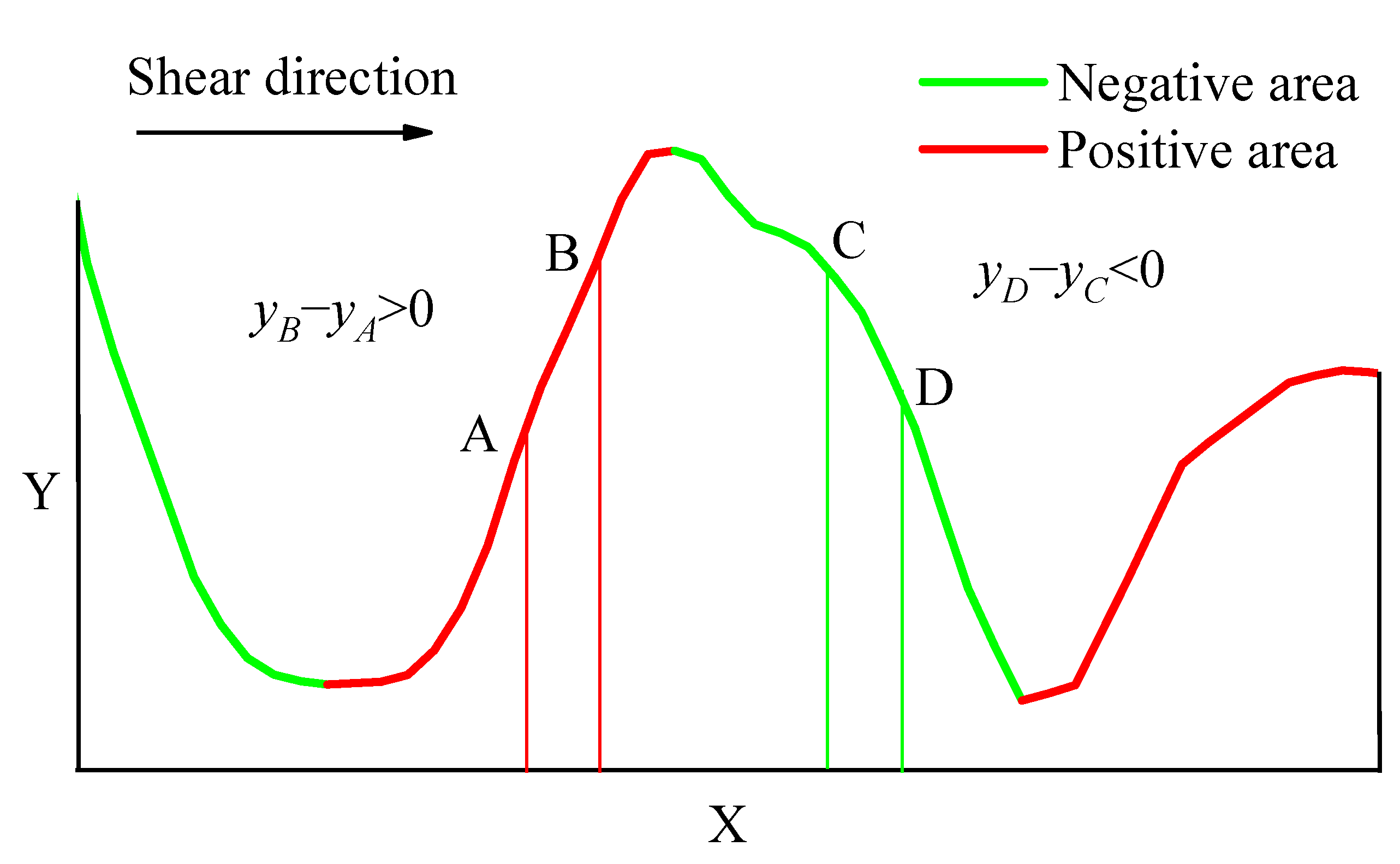
Modified Root Mean Square Z2′
The roughness of rock joints is an anisotropic property. Variation in the shear direction may cause a change in the shear strength of the joint surface. The profile is divided into positive and negative areas along the shear direction to account for the directional dependencies of JRC (Figure 5). Zhang et al. [3] suggested that the positive area should be considered in the process of determining joint roughness in the shear direction. Therefore, the modified root mean square of the first deviation of the profile was obtained.
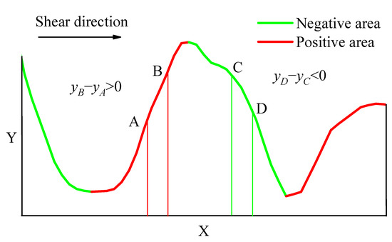
Figure 5.
Positive and negative areas in the shear direction.
4.2. Size Effect of Regular Sampling Interval
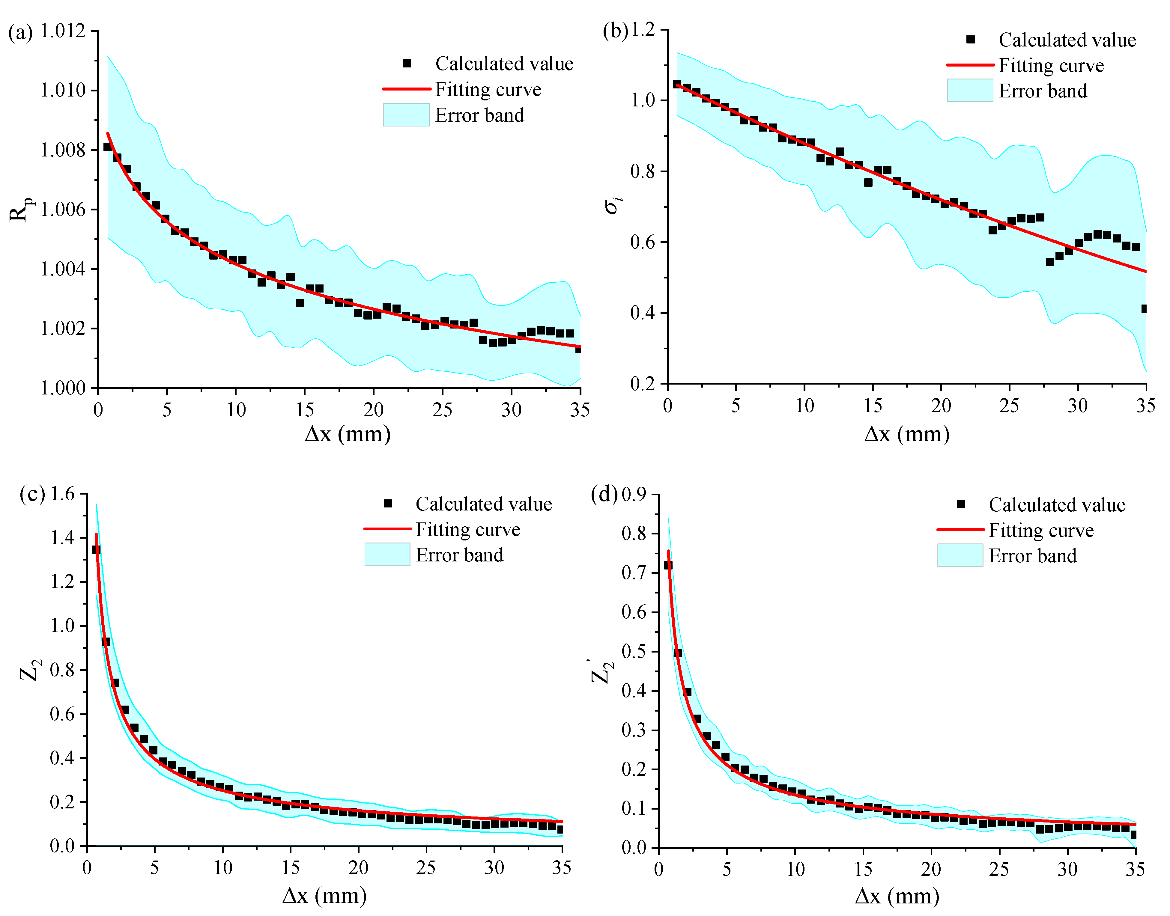
There are many contradictions in the existing research results regarding the size effect. Most scholars believe that there is a negative correlation between the sampling interval and JRC [19], while the roughness characterization method proposed by Ban et al. [20] shows a positive size effect, a negative size effect and no size effect in a certain direction. The size effect of roughness is linked to the characteristics of the joint surface itself and the shear direction. The above equations were used to calculate the roughness of the 14 profiles in the shear direction. The average roughness and variance are shown in Figure 6. It is obvious that the parameters Rp, σi, Z2 and Z2′ decreased with the increase in sampling interval, and eventually stabilized, showing a negative size effect. As the sampling interval increased, the roughness parameters reduced rapidly and finally stabilized gradually. As the existing roughness estimation methods are sensitive to the sampling interval (Δx), it is extremely important to study the relationship between the sampling interval and roughness in order to determine the maximum sampling interval. Huang et al. [22] established an empirical formula of JRC, Z2 and Δx.
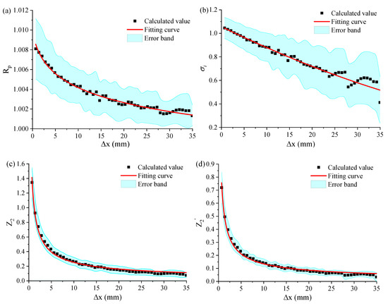
Figure 6.
Relationships between roughness parameters with sampling interval. (a) Rp; (b) σi; (c) Z2; (d) Z2′.
Unfortunately, it is difficult to determine the maximum sampling interval directly through the above empirical formula. Yong et al. [24] proposed a method of Fourier series reconstruction of the roughness profiles to determine the maximum sampling interval, although this approach is very cumbersome.
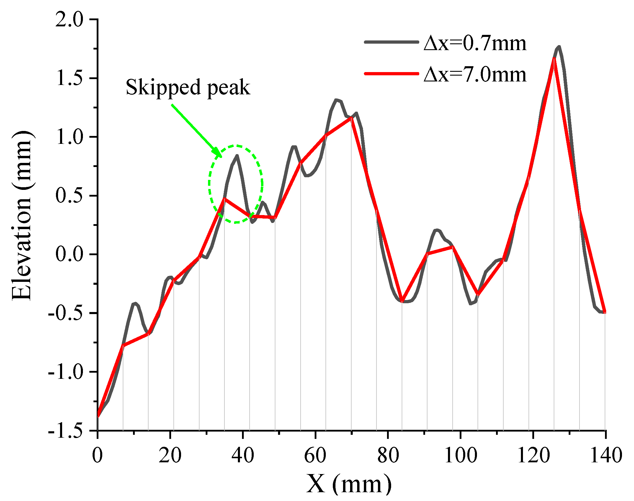
As shown in Figure 7, the fluctuation of the original profile L1 can be better reflected when the sampling interval is set as Δx = 0.7 mm; meanwhile, the sampling point skips a part of the peak or trough on the profile when the sampling interval is set as Δx = 7.0 mm. Consequently, the equal-spacing sampling method modifies the geometrical morphology of the original profile. The roughness estimation error becomes larger and larger with the increase in sampling interval. The threshold value of the sampling interval suggested in previous studies obtained from stabilized roughness in fact filters the influence of the secondary fluctuations in the original profile on the roughness evaluation. However, these secondary fluctuations play a significant role in the shearing process of the joint surface.

Figure 7.
Profiles of L1 with different sampling intervals.
4.3. Non-Equal Interval Sampling Method
In order to ensure the geometrical morphology of the original profile to the utmost extent, a non-equal interval sampling method is proposed. When the non-equal interval sampling method is applied, the sampling frequency should be increased where the curvature is large, which can be reduced, and the sampling spacing should be increased in places with small curvature. Mathematically, if the joint profile can be expressed by the equation (Figure 8), for any point M on the profile line where , the curvature radius is:
The curvature K and the radius of curvature R are both greater than 0 when , indicating that the arc is curved upward or the circle of curvature is above the arc. Conversely, this implies that the arc is curved downward or the circle of curvature is below the arc.
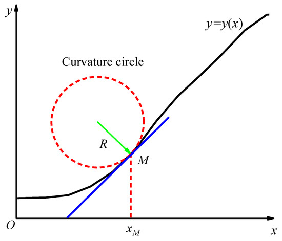
Figure 8.
Curvature radius of point M on the profile line.
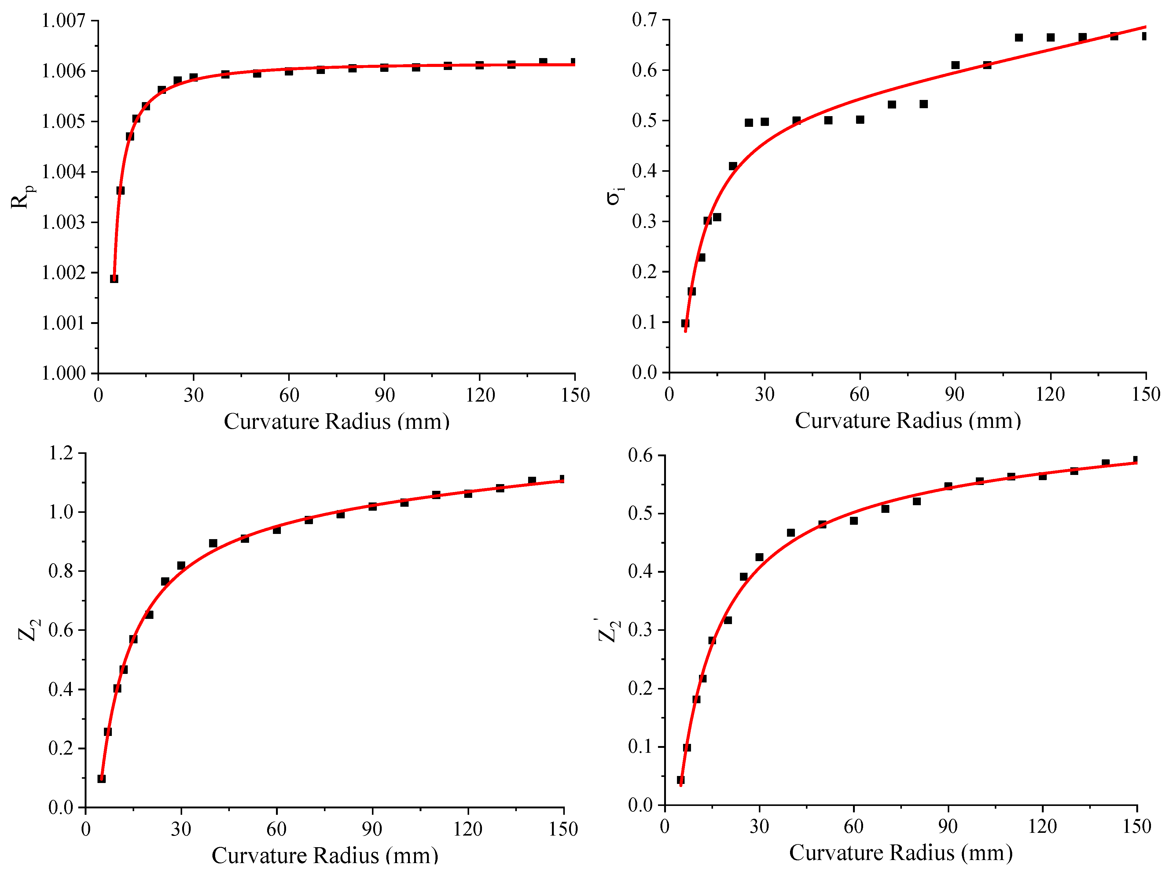
The curvature radius between adjacent points was calculated along the shear direction after obtaining the point clouds of the rock joints by 3D laser scanning. Different curvature radius thresholds R0 were applied. The coordinate data were recorded and saved if the calculated curvature radius R < R0. Otherwise, the data of this point were not recorded. The values of the four roughness parameters mentioned above under different curvature radius thresholds were calculated using this method (Figure 9). In the process of reducing the curvature radius threshold R0, the values of the parameters showed different degrees of reduction. However, the reduction in each parameter was trivial when R0 was between 150 mm and 30 mm, indicating that the roughness parameters are not sensitive to the variation in the curvature radius in this range. Contrarily, the roughness parameters decreased rapidly with the decrease in the curvature radius when R0 < 30 mm.
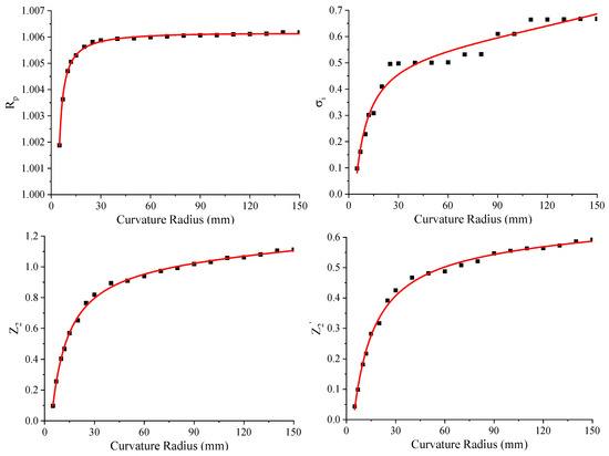
Figure 9.
Roughness under different curvature radius thresholds.
The following equation was adopted to determine the sampling frequency on the joint profile:
where the square bracket represents rounding, f is the sampling frequency, and Ki is the curvature at the i-th point on the profile line; Δx0 relates to the accuracy of the 3D laser scanner.
Equation (8) implies that the sampling frequency of a local curve on the profile is close to 0 when its curvature satisfies . As a consequence, points on this local curve can be skipped and have almost no influence on the roughness estimation, while the geometry information of a point will be recorded for roughness calculation where the sampling frequency .
Figure 10 shows the original profile, non-equal sampling frequency and its profile of L1, indicating that the geometrical morphology of the profile obtained using Equation (8) is almost the same as the original profile. Roughness values calculated by the profile using the proposed non-equal interval sampling method are listed in Table 1. The relative errors of Rp, Z2 and Z2′ are, respectively, 0.01%, −1.15% and 0.60%, while the angle standard deviation σi has an error of 50.10%. The roughness values calculated from the original profile and the non-equidistant profile are in good agreement. Numerous methods, including UAV aerial surveys and three-dimensional laser scanning, can obtain massive point cloud data. The processing of these point cloud data is a huge challenge in terms of computer storage and computing performance. However, the amount of data required by the proposed non-equal interval sampling method is only 54.7% of the original data. In other words, the non-equidistant roughness evaluation method can greatly reduce the amount of data to improve the efficiency of data processing, but has little effect on the overall roughness.
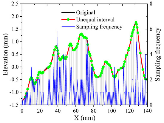
Figure 10.
Non-equidistant sampling frequency and its profiles of L1.

Table 1.
Relative error of roughness calculation using non-equidistant methods.
4.4. Roughness Anisotropy
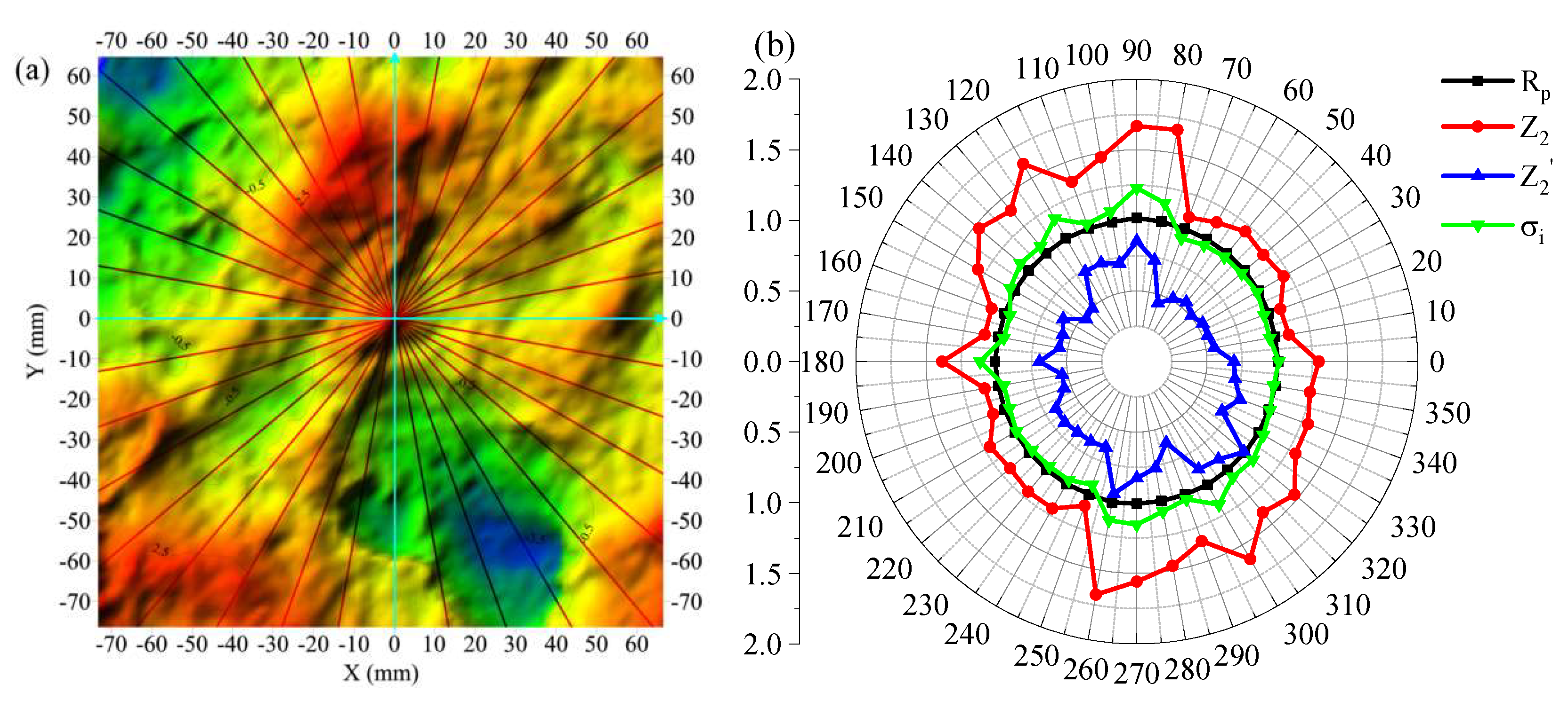
The anisotropy of roughness severely affected the shear failure mode of the rock joints. Based on the aforementioned four roughness evaluation parameters, the roughness anisotropy of the joint surface is discussed. According to the proposed non-equal interval sampling method, the four roughness evaluation parameters were calculated by Equations (1)–(5). In total, 36 directional profiles were extracted from 0° to 360° with an interval of 10° to analyze the roughness anisotropy of the joint surface (Figure 11a), where the x axis is the direction of 0° and the y axis is the direction of 90°. Obtained radar plots of the four roughness parameters are presented in Figure 11b.
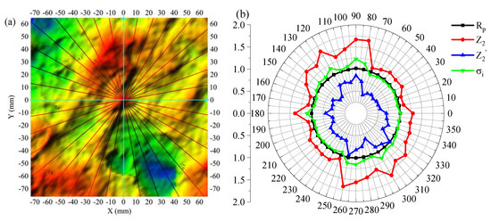
Figure 11.
The anisotropy of roughness. (a) Profiles along circumferential directions; (b) Roughness in radar plot.
To quantitatively characterize the roughness anisotropy of joint surfaces, a parameter AAHD considering the roughness characteristics of different shear directions was proposed by Ban et al. [20]. Using a method similar to that of Ban et al. [20], the anisotropy of the roughness parameter (ARP) is defined as:
where RPi is the roughness for the i-th analysis direction of a specific evaluating parameter, and four parameters Rp, σi, Z2 and Z2′ are used in this paper; RPave is the average value of RPi of all analysis directions, and n is the total number of analysis directions. The roughness anisotropy parameter ARP is composed of RPi, which can reflect the shear mechanism and takes into consideration the roughness characteristics of the joint surface in all shear directions; thus, it is more reasonable and comprehensive. When ARP = 0, the roughness of the joint surface is isotropic, and when ARP > 0, the roughness of the joint surface is anisotropic. The larger the value is, the more significant the anisotropic character.
The anisotropy indexes of the four roughness parameters Rp, σi, Z2 and Z2′ are 0.004, 0.078, 0.187 and 0.137, respectively. The calculation results show that Z2 and Z2′ can accurately reflect the anisotropy of the joint surface, while the anisotropy of Rp is the least obvious, followed by σi. It can be seen from Figure 11a that there are several obvious ridges on the joint surface with an attitude of around 50°~70°. The calculated roughness of σi, Z2 and Z2′ in this direction is the smallest, indicating that the resistance is minimal when the joint surface is sheared along the direction of 50°~70°. However, the direction of 80°~140° intersects the direction of the ridge with a large angle, and the calculated roughness is relatively large, indicating that the joint surface receives the greatest resistance when shearing in this direction.
5. Shear Failure Mechanism of Rock Joints
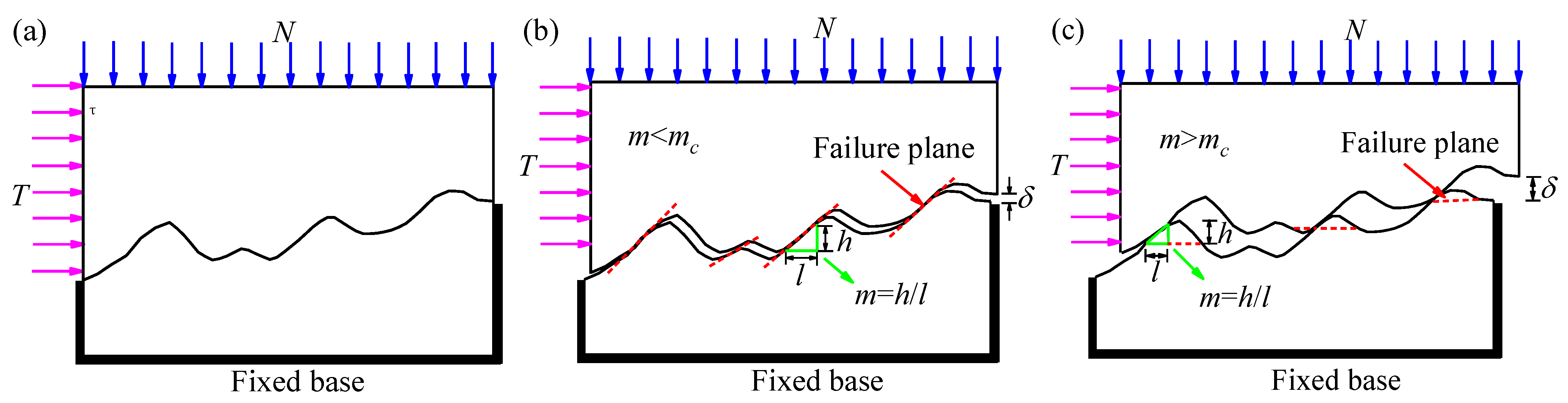
Two failure modes may exist in the rock joints in the process of shearing, namely dilatancy failure and non-dilatancy failure (shear fracture) (Figure 12). Ban et al. [14] defined the critical aspect ratio mc:
where φf is the internal friction angle of an intact rock.
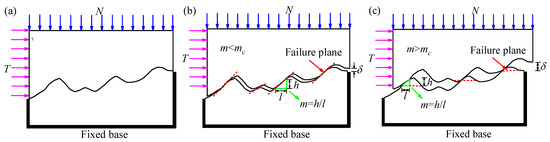
Figure 12.
Failure modes of rock joints during direct shear test. (a) Joint matching; (b) Dilatancy failure; (c) Fracture failure. The aspect ratio of the local convex area is m = h/l, and the dilatancy is δ.
The method proposed by Kwon et al. [34] was used to calculate the shear stress of the joint surface:
where cf is the cohesion of an intact rock and σn is the normal stress. m = h/l is the aspect ratio of the local convex area (Figure 12).
As shown in Figure 5 and Figure 12, the protruding part of the joint surface along the shear direction is beneficial to improve the shear strength. The roughness profile was divided into a positive area (yB − yA > 0) and a negative area (yD − yC < 0) along the shear direction (Figure 5). The shear stress was 0 on the negative region during the shearing process, i.e., τ = 0. Two failure modes existed on the positive region in the process of shearing (Figure 12). When m is less than mc, the shear strength increases linearly with m. When m is greater than mc, the shear strength remains unchanged.
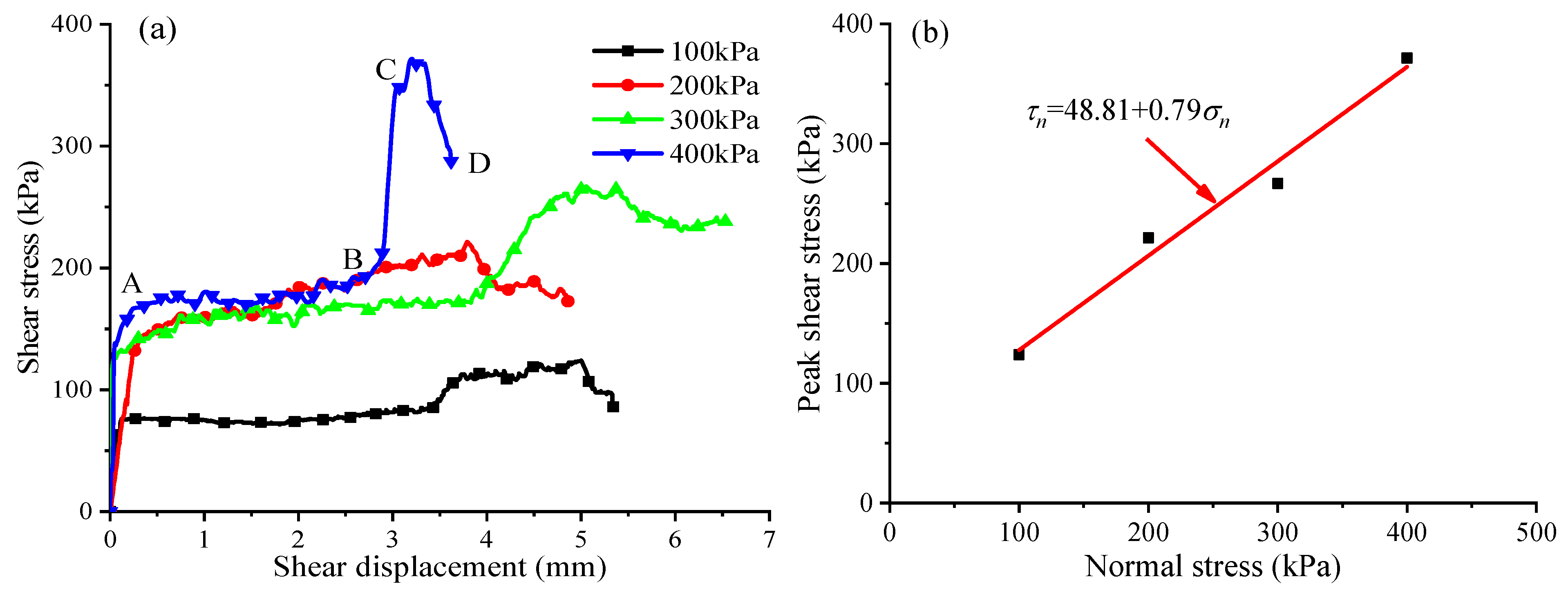
The variation in shear stress with shear displacement on the joint surface is displayed in Figure 13a, and the relationship between peak shear strength and normal stress (Figure 13b) was obtained. The apparent cohesion and internal friction angle of the rock joint were, respectively, cf = 48.81 kPa and φf = 38.26°. Figure 13a illustrates that, under any normal stress conditions, an increase in shear stress occurs twice in the process of shearing. The variation in shear stress with shear displacement can be divided into several stages. The shear stresses increased rapidly at the initial stage of the test (OA stage), and they were almost unchanged or only slightly increased at stage AB; the shear stress increased again at stage BC and finally decreased (CD stage).

Figure 13.
Results of direct shear test. (a) The variation in shear stress with shear displacement; (b) The relationship between peak shear strength and normal stress.
Complex geo-technical response should be faced with the progress of engineering construction because of sudden change of failure pattern and formation modulus [35]. The variation in shear stress with shear displacement may be related to the geometric characteristics of the joint surface. The shear strength on the rough surface was triggered in two stages. The first stage occurred at the beginning of the test. Initially, the inferior block and the superior block of the rock joints matched well (shown in Figure 12a). After a slight displacement of the sample, the friction strength between the upper and lower rocks could be quickly activated due to the dilatancy and slip effect. The shear stress was essentially unchanged or only slightly increased when the sliding friction strength of the structural surface was fully adjusted. The rock blocks suffered from the resistance of the protruding parts on the uneven surface after sliding for a certain distance, forming an interlocking effect. As a consequence, the shear strength was activated again because of the interlocking effect. The shear stress was quickly reduced if the interlocking effect disappeared owing to the shearing destruction of these protruding parts on the roughness surface.
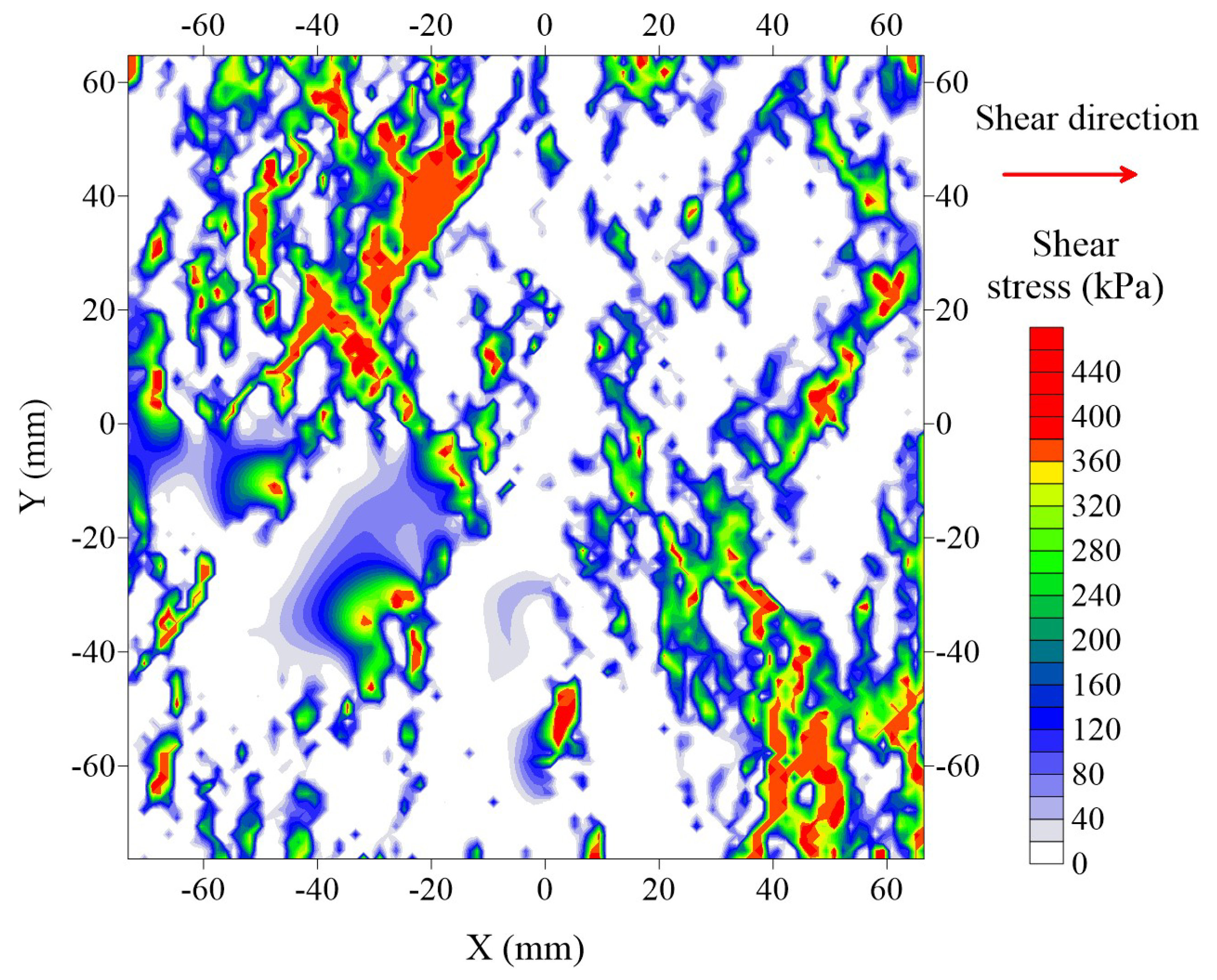
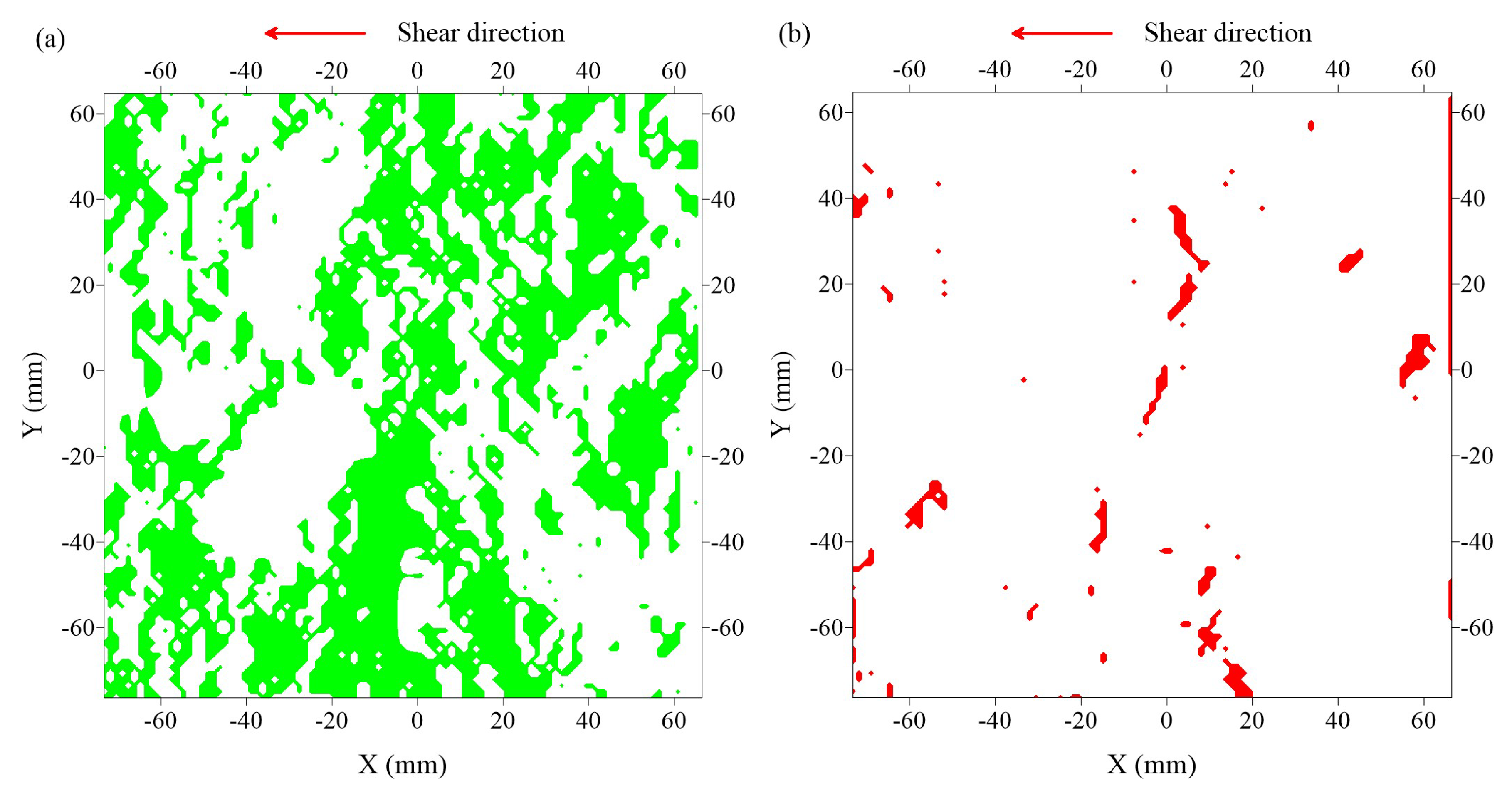
The shear stress distribution along different shear directions was calculated by Equation (11) for the normal stress σn = 400 kPa. Shear stress distribution for shearing in the positive direction of the x axis is shown in Figure 14, where white indicates that no shear stress was exerted in this area during the shearing process. The calculation result reveals that the protruding parts on the roughness surface contributed to the shear strength. As mentioned previously, two different failure modes were exhibited on the joint surface during the shearing process. The dilatancy failure area and fracture failure area for shearing in the positive direction of the x axis are shown in Figure 15. Accompanying the appearance of dilatancy, a large area on the rough surface expressed a certain degree of slip (Figure 15a). Stress concentration occurred when the upper and lower blocks of the roughness surface slipped to a certain extent, resulting in shear fracture failure of the protruding parts on the roughness surface due to shear stress greater than their shear strength (Figure 15b).
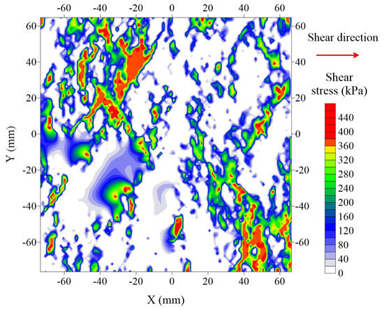
Figure 14.
Shear stress distribution for shearing in the positive direction of the x axis.
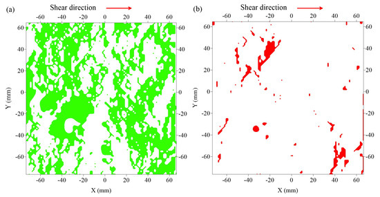
Figure 15.
Two types of failure areas for shearing in the positive direction of the x axis. (a) Dilatancy failure area; (b) Fracture failure area.
In order to reflect the influence of roughness anisotropy on shear strength, the shear stress distribution for shearing in the negative direction of the x axis was calculated under the same conditions (Figure 16). The dilatancy failure area and fracture failure area in this situation were discussed (Figure 17). Comparing the shear stress distribution on the joint surface during shearing along the positive and negative directions of the x axis, it was found that the shear stress distribution was significantly different by changing the shear direction. There were regions with failure from dilatancy or shear fracture by shearing in the positive direction, while no shear stress was exerted in these regions for shearing in the opposite direction. Significant differences in the shear strength of the joint surface were exhibited in the two situations. However, only the modified root mean square parameter Z2′ among the four roughness evaluation parameters selected in this paper can consider the failure mechanism in the case of changing the shearing direction of the rock joints.
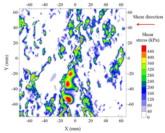
Figure 16.
Shear stress distribution for shearing in the negative direction of the x axis.
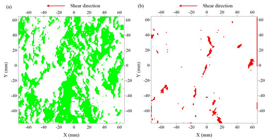
Figure 17.
Two types of failure areas for shearing in the negative direction of the x axis. (a) Dilatancy failure area; (b) Fracture failure area.
6. Conclusions
Influences of point cloud noise and the non-stationary nature of joints on roughness evaluation are discussed, and a method to remove the non-stationary feature of point clouds is proposed.
The scale effect and anisotropy of roughness for a uniform sampling interval are investigated by four parameters Rp, σi, Z2 and Z2′, exhibiting an obvious negative size effect. The reason for the scale effect of joint surface roughness is that the regular sampling interval method changes the geometrical morphology of the original profile, thereby ignoring the contribution of secondary fluctuations to roughness.
A non-equal interval sampling method and an equation for determining the sampling frequency on the roughness profile are proposed, which can successfully maintain the morphological characteristics of the original profile and reduce the data processing cost.
Direct shear tests under constant normal load (CNL) conditions are carried out to study the influence of roughness anisotropy on the shear failure mechanism of rock joints. The shear stress is found to be determined by the failure mechanisms of dilatancy and shear fracture on the roughness of the joint.
The distributions of shear stress, dilatancy and fracture areas on the roughness of the joint in different shear directions are calculated theoretically. Results show that the anisotropy and failure mechanism of joint roughness can be well characterized by the modified root mean square parameter Z2′.
The research results are helpful for understanding the influences of roughness sampling interval and anisotropy on the shear failure mechanism of the rock joint surface.
Author Contributions
Visualization and writing—original draft preparation, F.C.; conceptualization, methodology and supervision, H.Y.; investigation and data collection, Y.Y.; validation, reviewing, editing and funding acquisition, D.W. All authors have read and agreed to the published version of the manuscript.
Funding
This research was funded by the National Natural Science Foundation of China, grant number 42002280; the Science and Technology Program of Guizhou Province, grant number [2019]1056; and the Geological Scientific Research Project of the Bureau of Geology and Mineral Exploration and Development Guizhou Province, grant number [2015]18.
Institutional Review Board Statement
Not applicable.
Informed Consent Statement
Not applicable.
Data Availability Statement
Data are contained within the article.
Conflicts of Interest
The authors declare no conflict of interest.
References
- Faraji, M.; Rezagholilou, A.; Ghanavati, M.; Kadkhodaie, A.; Wood, D.A. Breakouts derived from image logs aid the estimation of maximum horizontal stress: A case study from Perth Basin, Western Australia. Adv. Geo-Energy Res. 2021, 5, 8–24. [Google Scholar] [CrossRef]
- Rullière, A.; Peyras, L.; Breul, P. Influence of Roughness on the Apparent Cohesion of Rock Joints at Low Normal Stresses. J. Geotech. Geoenviron. Eng. 2020, 146, 04020003. [Google Scholar] [CrossRef]
- Zhang, G.; Karakus, M.; Tang, H.; Ge, Y.; Zhang, L. A new method estimating the 2D Joint Roughness Coefficient for discontinuity surfaces in rock masses. Int. J. Rock Mech. Min. Sci. 2014, 72, 191–198. [Google Scholar] [CrossRef]
- Anyim, K.; Gan, Q. Fault zone exploitation in geothermal reservoirs: Production optimization, permeability evolution and induced seismicity. Adv. Geo-Energy Res. 2020, 4, 1–12. [Google Scholar] [CrossRef] [Green Version]
- Barton, N.; Choubey, V. The shear strength of rock joints in theory and practice. Rock Mech. Felsmech. Mec. Roches 1977, 10, 1–54. [Google Scholar] [CrossRef]
- Power, W.L.; Tullis, T.E. Euclidean and fractal models for the description of rock surface roughness. J. Geophys. Res. 1991, 96, 415–424. [Google Scholar] [CrossRef]
- Sayles, R.S.; Thomas, T.R. The spatial representation of surface roughness by means of the structure function: A practical alternative to correlation. Wear 1977, 42, 263–276. [Google Scholar] [CrossRef]
- Brown, S.; Scholz, C. Broad Bandwidth Study of the Topography of Natural Rock Surface. J. Geophys. Res. 1985, 90, 12575–12582. [Google Scholar] [CrossRef]
- Ünlüsoy, D.; Süzen, M. A new method for automated estimation of joint roughness coefficient for 2D surface profiles using power spectral density. Int. J. Rock Mech. Min. Sci. 2020, 125, 104156. [Google Scholar] [CrossRef]
- Aslam, M. A New Method to Analyze Rock Joint Roughness Coefficient Based on Neutrosophic Statistics. Measurement 2019, 146, 65–71. [Google Scholar] [CrossRef]
- Magsipoc, E.; Zhao, Q.; Grasselli, G. 2D and 3D Roughness Characterization. Rock Mech. Rock Eng. 2020, 53, 1495–1519. [Google Scholar] [CrossRef]
- Chen, S.; Zhu, W.; Yu, Q.; Liu, X. Characterization of Anisotropy of Joint Surface Roughness and Aperture by Variogram Approach Based on Digital Image Processing Technique. Rock Mech. Rock Eng. 2015, 49, 855–876. [Google Scholar] [CrossRef]
- Hu, S.; Huang, L.; Chen, Z.; Ji, Z.; Liu, Z. Effect of Sampling Interval and Anisotropy on Laser Scanning Accuracy in Rock Material Surface Roughness Measurements. Strength Mater. 2019, 51, 678–687. [Google Scholar] [CrossRef]
- Ban, L.; Zhu, C.; Qi, C.; Tao, Z. New roughness parameters for 3D roughness of rock joints. Bull. Eng. Geol. Environ. 2018, 78, 4505–4517. [Google Scholar] [CrossRef]
- Zhao, Z.; Guo, T.; Li, S.; Wu, W.; Yang, Q.; Chen, S. Effects of joint surface roughness and orientational anisotropy on characteristics of excavation damage zone in jointed rocks. Int. J. Rock Mech. Min. Sci. 2020, 128, 104265. [Google Scholar] [CrossRef]
- Yong, R.; Huang, L.; Hou, Q.; Du, S. Class Ratio Transform with an Application to Describing the Roughness Anisotropy of Natural Rock Joints. Adv. Civ. Eng. 2020, 2020, 5069627. [Google Scholar] [CrossRef]
- Abolfazli, M.; Fahimifar, A. An investigation on the correlation between the joint roughness coefficient (JRC) and joint roughness parameters. Constr. Build. Mater. 2020, 259, 120415. [Google Scholar] [CrossRef]
- Azinfar, M.; Ghazvinian, A.; Nejati, H. Assessment of scale effect on 3D roughness parameters of fracture surfaces. Eur. J. Environ. Civ. Eng. 2016, 23, 1–28. [Google Scholar] [CrossRef]
- Bao, H.; Zhang, G.; Lan, H.; Yan, C.; Xu, J.; Xu, W. Geometrical heterogeneity of the joint roughness coefficient revealed by 3D laser scanning. Eng. Geol. 2019, 265, 105415. [Google Scholar] [CrossRef]
- Ban, L.; Qi, C.; Chen, H.; Yan, F.; Ji, C. A New Criterion for Peak Shear Strength of Rock Joints with a 3D Roughness Parameter. Rock Mech. Rock Eng. 2020, 53, 1755–1775. [Google Scholar] [CrossRef]
- Mo, P.; Li, Y. Estimating the three-dimensional joint roughness coefficient value of rock fractures. Bull. Eng. Geol. Environ. 2017, 78, 857–866. [Google Scholar] [CrossRef] [Green Version]
- Huang, M.; Xia, C.; Sha, P.; Ma, C.; Du, S. Correlation between the Joint Roughness Coefficient and Rock Joint Statistical Parameters at Different Sampling Intervals. Adv. Civ. Eng. 2019, 2019, 1643842. [Google Scholar] [CrossRef] [Green Version]
- Du, S.; Gao, H.; Hu, Y.; Huang, M.; Zhao, H. A New Method for Determination of Joint Roughness Coefficient of Rock Joints. Math. Probl. Eng. 2015, 2015, 634573. [Google Scholar] [CrossRef]
- Yong, R.; Ye, J.; Li, B.; Du, S. Determining the maximum sampling interval in rock joint roughness measurements using Fourier series. Int. J. Rock Mech. Min. Sci. 2018, 101, 78–88. [Google Scholar] [CrossRef]
- Yong, R.; Fu, X.; Huang, M.; Liang, Q.; Du, S. A rapid field measurement method for the determination of Joint Roughness Coefficient of large rock joint surfaces. KSCE J. Civ. Eng. 2017, 22, 101–109. [Google Scholar] [CrossRef]
- Huan, J.; He, M.; Zhang, Z.; Li, N. A New Method to Estimate the Joint Roughness Coefficient by Back Calculation of Shear Strength. Adv. Civ. Eng. 2019, 2019, 7897529. [Google Scholar] [CrossRef] [Green Version]
- Renaud, S.; Saichi, T.; Bouaanani, N.; Miquel, B.; Quirion, M. Roughness Effects on the Shear Strength of Concrete and Rock Joints in Dams Based on Experimental Data. Rock Mech. Rock Eng. 2019, 52, 3867–3888. [Google Scholar] [CrossRef]
- Ge, Y.; Lin, Z.; Tang, H.; Zhao, B.; Chen, H.; Xie, Z.; Du, B. Investigation of the effects of nonstationary features on rock joint roughness using the laser scanning technique. Bull. Eng. Geol. Environ. 2020, 79, 3163–3174. [Google Scholar] [CrossRef]
- Bitenc, M.; Kieffer, D.; Khoshelham, K. Range Versus Surface Denoising of Terrestrial Laser Scanning Data for Rock Discontinuity Roughness Estimation. Rock Mech. Rock Eng. 2019, 52, 3103–3117. [Google Scholar] [CrossRef] [Green Version]
- Li, Y.; Zhang, Y. Quantitative estimation of joint roughness coefficient using statistical parameters. Int. J. Rock Mech. Min. Sci. 2015, 100, 27–35. [Google Scholar] [CrossRef] [Green Version]
- El-Soudani, S.M. Profilometric analysis of fractures. Metallography 1978, 11, 247–336. [Google Scholar] [CrossRef]
- Yu, X.; Vayssade, B. Joint profiles and their roughness parameters. Int. J. Rock Mech. Min. Sci. Geomech. Abstr. 1991, 28, 333–336. [Google Scholar] [CrossRef]
- Myers, N.O. Characterization of surface roughness. Wear 1962, 5, 182–189. [Google Scholar] [CrossRef]
- Kwon, T.H.; Hong, E.S.; Cho, G.C. Shear behavior of rectangular-shaped asperities in rock joints. KSCE J. Civ. Eng. 2010, 14, 323–332. [Google Scholar] [CrossRef]
- Li, Y.; Liu, C.; Liu, L.; Sun, J.; Liu, H.; Meng, Q. Experimental study on evolution behaviors of triaxial-shearing parameters for hydrate-bearing intermediate fine sediment. Adv. Geo-Energy Res. 2018, 2, 43–52. [Google Scholar] [CrossRef] [Green Version]


Publisher’s Note: MDPI stays neutral with regard to jurisdictional claims in published maps and institutional affiliations. |
© 2021 by the authors. Licensee MDPI, Basel, Switzerland. This article is an open access article distributed under the terms and conditions of the Creative Commons Attribution (CC BY) license (https://creativecommons.org/licenses/by/4.0/).