Active Damping Injection Output Voltage Control with Dynamic Current Cut-Off Frequency for DC/DC Buck Converters

Abstract

With regard to DC/DC buck converter applications, the objective of this study is to expand the admissible range of the output voltage cut-off frequency while lowering the steady-state current cut-off frequency as possible. This study fortifies the inner loop by incorporating the novel subsystems such as an auto-tuner (for the dynamic current cut-off frequency) and active damping injection invoking the pole-zero cancellation nature with the particular designed feedback gain structure. The outer loop active damping control renders the closed-loop speed transfer function to be a first-order low-pass filter with the cooperation of the specially structured design parameters; in addition, it provides time-varying disturbance attenuation. The experimental results obtained for a 3-kW buck converter validate the feasibility of the proposed technique by showing a $34\%$ performance enhancement (at least) compared with the recent active damping controller.

1. Introduction

Battery-based industrial applications (including drones, electrical vehicles, and mobile robots) require high-quality DC power supply systems to ensure improved reliability during operation [1,2,3]. To address these industrial needs, DC/DC power converters are considered to be a reasonable solution. These converters are equipped with devised that provide major advantages, such as power factor correction. Moreover, a carefully designed feedback controller can dramatically improve the closed-loop robustness to variations in the load and operating conditions [4,5,6].

The cascade-type control strategy is typically adopted to ensure high-performance DC/DC power conversion, and the inner and outer loops should regulate the inductor current and output capacitor-side voltage, respectively [7,8]. The introduction of a fast current loop provides practical advantages. First, it improves the output voltage control performance by kicking off the unstable zero through the high-current loop cut-off frequency settings. Secondly, it limits the inductor current by using software to regulate the current reference signal obtained from the outer loop controller. To ahieve the two above-mentioned benefits, proportional-integral (PI) controllers were mainly been adopted for each loop. The selected PI gains assign the cut-off frequencies for the current and voltage loops to satisfy the desired closed-loop performance and robustness described in the frequency domain. Typically, the current cut-off frequency is set to be greater than that of the voltage loop, which makes the current loop faster compared with the voltage loop. This closed-loop setting may limit the output voltage control performance based on the current cut-off frequency specification. Increasing the current cut-off frequency to increase the admissible output voltage cut-off frequency can result in the increase of the current ripples or even instability [7,9,10]. To limit the current cut-off frequency, a feed-forward compensation technique was developed with consideration to the converter current dynamics. This technique requires the true converter inductance and capacitance values to vary in accordance with the operating conditions [11]. The resulting closed-loop accuracy can be greatly improved by adopting additional novel online parameter identifiers (as in [12,13]).

There are several novel methods for ensuring the high output voltage control performance while avoiding the increase of the current cut-off frequency: for example, predictive [14], deadbeat [15], adaptive [16], sliding mode [17], backstepping [18], and nonlinear robust methods [19]. These methods achieve true converter parameter dependence level reduction for the feed-forward compensation terms. However, the control actions keep the current cut-off frequency constant, although it must be increased to achieve rapid output voltage dynamics. The recently proposed cascade-type feedback linearization (FL) controller stabilizes the current and voltage at the desired values, and the optimal feedback gains determine the constant current and voltage cut-off frequencies [20]. The differential inclusion technique based on the discontinuous switching function has been applied to ensure the global tracking property without controlled error integrators and a pulse-wide modulation (PWM) process [21]. The state-feedback controllers collaborate with the disturbance observer (DOB) used for the feed-forward compensator to stabilize the error dynamics; the feasibility of this method has been experimentally demonstrated [22,23]. The recent cascade-type proportional current and voltage controller systematically adopts nonlinear DOBs in the feed-forward loop with a rigorous proof of the offset-free property without control error integral actions [24]. Moreover, DOB-based energy-shaping controllers solve the parameter and load uncertainty problem by solving a partial differential equation, which ensures the removal of the steady-state error caused by the DOB dynamics. Model predictive control (MPC) has been proposed as a solution to the numerical solver dependence problem, which requires the true converter parameter and load information to ensure closed-loop optimality [25,26]. The analytic form self-tuner was incorporated into a DOB-based proportional-type outer loop controller to achieve a dynamic cut-off frequency [27]. For this technique, the constant inner loop cut-off frequency must be sufficiently increased to achieve the desired closed-loop performance. The voltage-derivative observer-based nonlinear PD controller removes the current feedback loop and solves the converter parameter and load dependence problem in the control and observer [28].

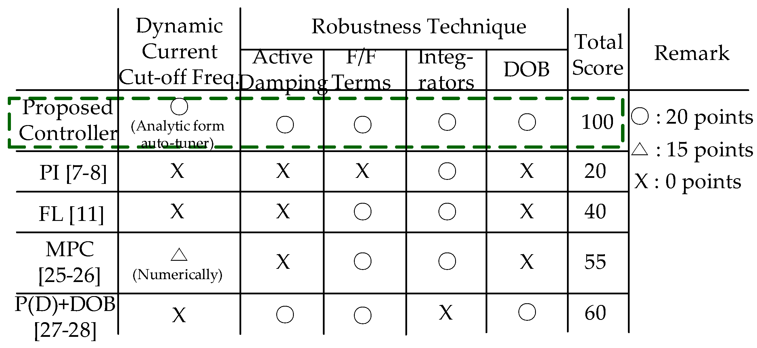
According to the literature review, the constant current-loop cut-off frequency assigned by the feedback gain must increase proportionally to the output voltage loop cut-off frequency to improve the transient dynamic performance, which is desirable only for the transient operations and can increase current ripple level and limit the closed-loop relative stability. The so-called “constant current cut-off frequency problem” corresponds to the main challenge faced by this study. This paper proposes a solution to this problem based on the following contributions:

• An online auto-tuner for the current cut-off frequency to be dynamically updated according to the transient and steady state operation mode;
• A DOB-based pole-zero cancellation current controller driven by the dynamic current cut-off frequency from the online auto-tuner;
• An active damping outer loop speed controller leading to a first-order closed-loop system with time-varying disturbance suppression capability by the active damping coefficient.

Convergence analysis is also carried out to highlight the contributions by investigating the closed-loop dynamics. A 3-kW DC/DC buck converter is used in the experiments to demonstrate that the proposed solution addresses the constant current cut-off frequency problem based on the dynamic current cut-off frequency from the online auto-tuner. The qualitative comparison results obtained by the above-mentioned studies are summarized in the table in Figure 1.

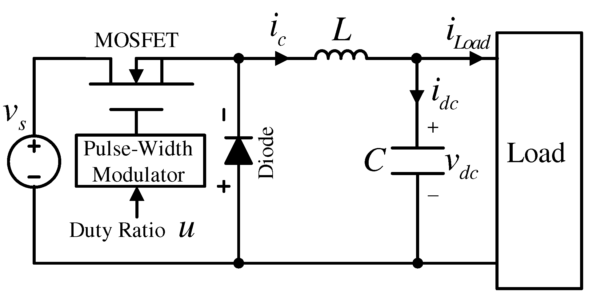
2. DC/DC Buck Converter Model

This study considers the standard DC/DC buck converter depicted in Figure 2, where the inductor current $i_c$ (in A) and output voltage $v_{dc}$ (in V) are the state variables excited by the duty ratio $u(\in [0,1\left]\right)$ (control input) applied to the switching device (MOSFET). The input source voltage and load current are represented as $v_s$ (in V) and $i_{Load}$ (in A), respectively. The application of the averaging technique to the circuit dynamics obtained from each switching state (ON and OFF) yields the second-order differential equations:

$$\begin{array}{ccc}\hfill L{\dot{i}}_c& =& -v_{dc}+v_{s}u,\hfill \end{array}$$

(1)

$$\begin{array}{ccc}\hfill C{\dot{v}}_{dc}& =& i_c+i_{Load},\forall t\ge 0,\hfill \end{array}$$

(2)

with L and C denoting the inductance and capacitance values, respectively.

The operation mode uncertainty validates the assumption stating that the true values of L and C and the load current $i_{Load}$ are unknown. Moreover, to reduce the number of sensors, the uncertainty of the input source voltage $v_s$ is also considered, except for its initial value $v_{s,0}$. Thus, the introduction of the nominal values $L_0$ and $C_0$ results in another version of the original converter dynamics (1) and (2):

$$\begin{array}{ccc}\hfill L_0{\dot{i}}_c& =& -v_{dc}+v_{s,0}u+{\overline{d}}_{i_c},\hfill \end{array}$$

(3)

$$\begin{array}{ccc}\hfill C_0{\dot{v}}_{dc}& =& i_c+d_{v_{dc}},\forall t\ge 0,\hfill \end{array}$$

(4)

with the lumped disturbances ${\overline{d}}_{i_c}$ and $d_{v_{dc}}$ to be treated as unknown time-varying signals, which are used to design the control law in the following sections. Notably, the equivalent series resistance (ESR) of the inductor and capacitor are also included in the perturbed disturbances $d_{i_c}$ and $d_{v_{dc}}$.

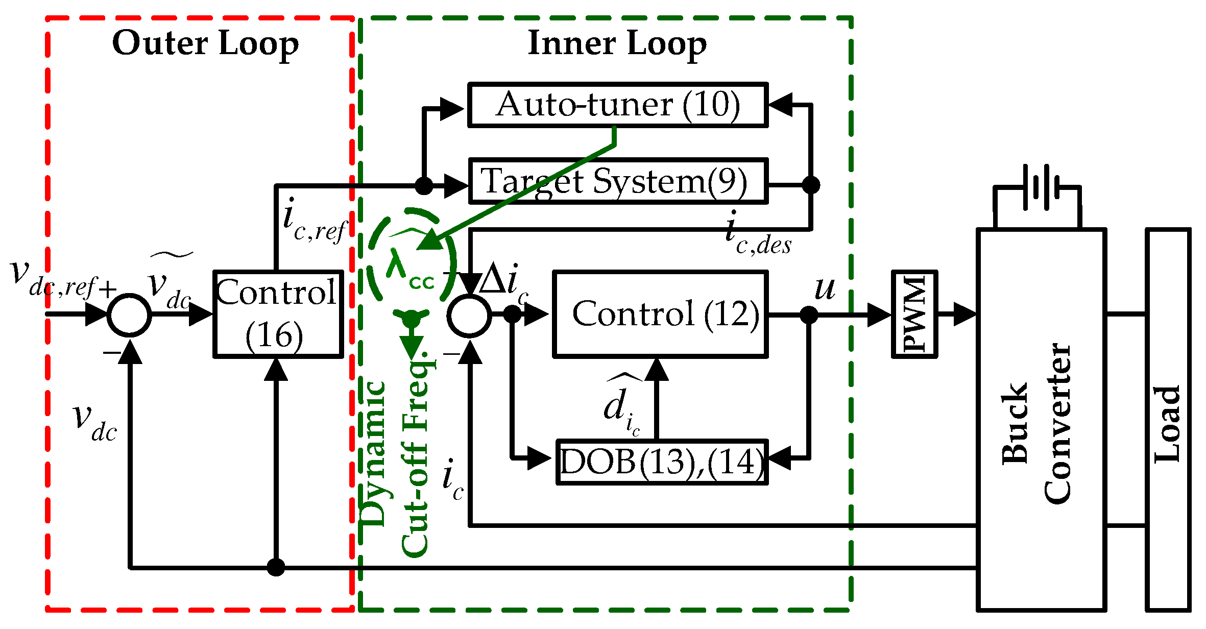
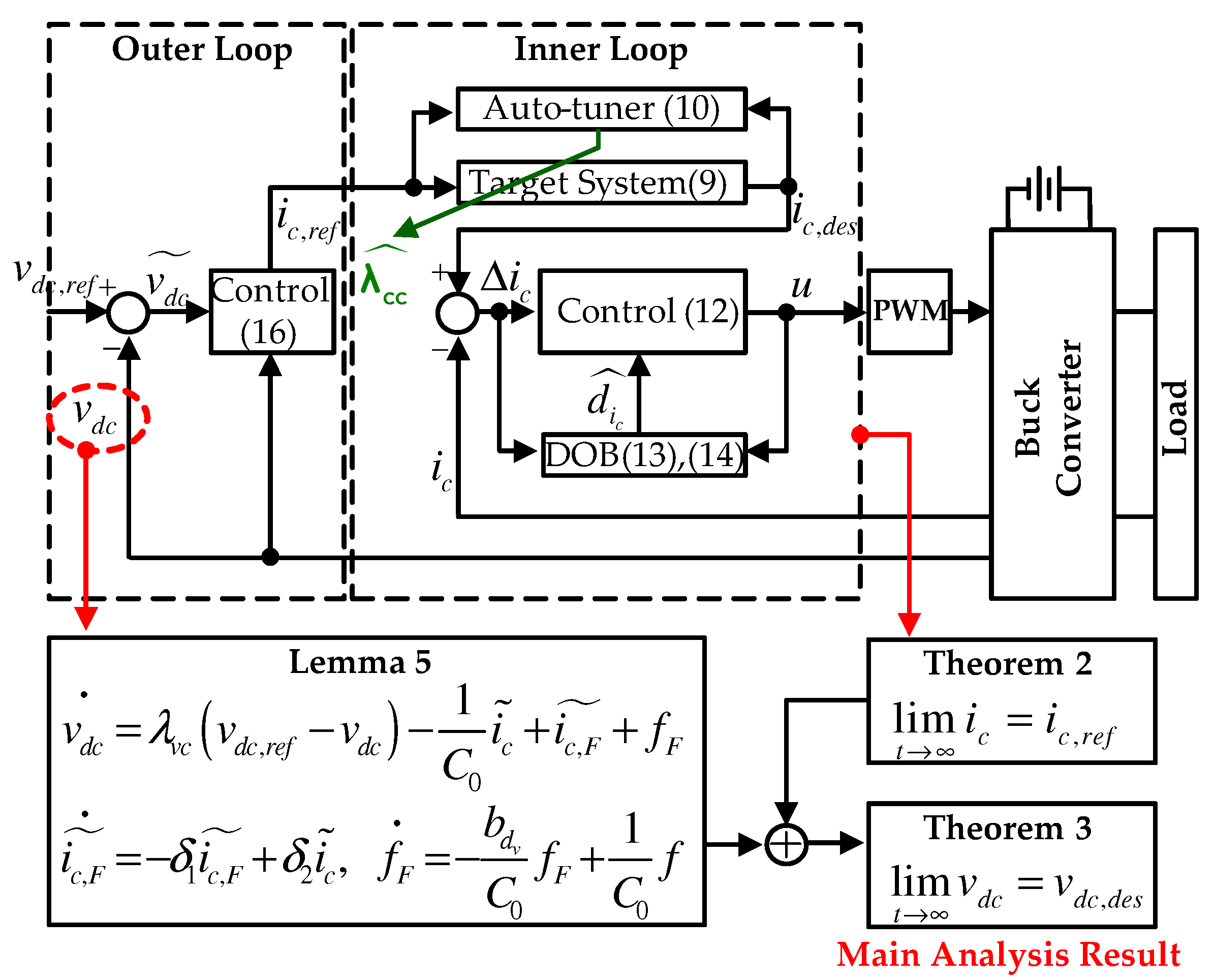
3. Proposed Control Algorithm

This section presents the cascade-type solution proposed for actual implementations as clearly as possible. The main results discussed in this section are presented in Figure 3. Section 3.1 and Section 3.2 give the corresponding detailed subsystem descriptions. The closed-loop analysis results are included in Section 4.

Before presenting the control algorithm, it is necessary to clarify the control objective of this study. Consider the desired output voltage trajectory $v_{dc,des}$ for a given reference $v_{dc,ref}$ with the Laplace transformations $V_{dc,des}\left(s\right)$ and $V_{dc,ref}\left(s\right)$, and define the target closed-loop transfer function as

$$\begin{array}{c}\hfill \frac{V_{dc,des}\left(s\right)}{V_{dc,ref}\left(s\right)}=\frac{{\lambda }_{vc}}{s+{\lambda }_{vc}},\forall s\in \mathbb{C},\end{array}$$

(5)

with the output voltage cut-off frequency ${\lambda }_{vc}=2\pi f_{vc}$ (${\lambda }_{vc}$ in rad/s, corresponding to $f_{vc}$ in Hz). Based on the desired system (5), the control objective is formulated as exponential convergence:

$$\begin{array}{c}\hfill \underset{t\to \infty }{lim}{v}_{dc}=v_{dc,des},\end{array}$$

(6)

where $v_{dc,des}$ denotes the inverse Laplace transform for the target system (5):

$$\begin{array}{c}\hfill {\dot{v}}_{dc,des}={\lambda }_{vc}(v_{dc,ref}-v_{dc,des}),\forall t\ge 0.\end{array}$$

(7)

3.1. Inner Loop for Current Control

3.1.1. Current Cut-off Frequency Auto-Tuner

For a given current reference $i_{c,ref}$ from the outer loop, define the target current dynamics as

$$\begin{array}{c}\hfill {\dot{i}}_{c,des}={\lambda }_{cc}(i_{c,ref}-i_{c,des}),\forall t\ge 0,\end{array}$$

(8)

with the current cut-off frequency ${\lambda }_{cc}=2\pi f_{cc}$ (${\lambda }_{cc}$ in rad/s corresponding to $f_{cc}$ in Hz); its transfer function is identical to (5) with the replacement ${\lambda }_{vc}$ with ${\lambda }_{cc}$. For a rapid output voltage transient response, the current cut-off frequency ${\lambda }_{cc}$ must to be proportional to the increase in ${\lambda }_{vc}$.

To boost the current cut-off frequency only during transient periods, a slight modification of the target current dynamics (8) with a dynamic current cut-off frequency ${\widehat{\lambda }}_{cc}$ is suggested as

$$\begin{array}{c}\hfill {\dot{i}}_{c,des}={\widehat{\lambda }}_{cc}(i_{c,ref}-i_{c,des}),\forall t\ge 0,\end{array}$$

(9)

with the auto-tuning rule for ${\widehat{\lambda }}_{cc}$:

$$\begin{array}{c}\hfill {\dot{\widehat{\lambda }}}_{cc}={\gamma }_{cc}({\tilde{i}}_{c,des}^2+{\sigma }_{cc}{\tilde{\lambda }}_{cc}),\forall t\ge 0,\end{array}$$

(10)

with the errors defined as ${\tilde{i}}_{c,des}=i_{c,ref}-i_{c,des}$ and ${\tilde{\lambda }}_{cc}={\lambda }_{cc}-{\widehat{\lambda }}_{cc}$, gains ${\gamma }_{cc}>0$ and ${\sigma }_{cc}>0$, and initial condition ${\widehat{\lambda }}_{cc}\left(0\right)={\lambda }_{cc}$.

Remark 1.

The nonlinear error term ${\tilde{i}}_{c,des}^2$ excites the dynamic current cut-off frequency ${\widehat{\lambda }}_{cc}$ whose boosting level is adjusted by ${\gamma }_{cc}>0$, and the stabilization term ${\tilde{\lambda }}_{cc}$ exponentially restores the boosted cut-off frequency to its initial value ${\widehat{\lambda }}_{cc}\left(0\right)={\lambda }_{cc}$ according to the decay rate ${\rho }_{cc}>0$. The corresponding formal analysis is presented in Section 4.

3.1.2. Control Law

The error $\Delta i_c=i_{c,des}-i_c$ is defined to accomplish the convergence ${lim}_{t\to \infty }{i}_c=i_{c,des}$ with $i_{c,des}$ representing the solution to the desired system (9). Then, it follows from (3) that

$$\begin{array}{ccc}\hfill L_0\Delta {\dot{i}}_c& =& L_0{\dot{i}}_{c,des}-L_0{\dot{i}}_c\hfill \\ & =& -v_{s,0}u+d_{i_c},\forall t\ge 0,\hfill \end{array}$$

(11)

with the re-defined lumped disturbance $d_{i_c}=L_0{\dot{i}}_{c,des}+v_{dc}-{\overline{d}}_{i_c}$. This study proposes the control law for stabilizing the open-loop system (11) as

$$\begin{array}{c}\hfill u=\frac{1}{v_{s,0}}((b_{d_L}+L_0{k}_{cc})\Delta i_c+b_{d_L}{k}_{cc}{\int }_0^t\Delta i_{c}d\tau +{\widehat{d}}_{i_c}),\end{array}$$

(12)

$\forall t\ge 0$, with gains $b_{d_L}>0$ and $k_{cc}>0$, where the DOB for updating ${\widehat{d}}_{i_c}$ is given by

$$\begin{array}{ccc}\hfill {\dot{z}}_{i_c}& =& -l_{i_c}{z}_{i_c}-l_{i_c}^2{L}_0\Delta i_c+l_{i_c}{v}_{s,0}u,\hfill \end{array}$$

(13)

$$\begin{array}{ccc}\hfill {\widehat{d}}_{i_c}& =& z_{i_c}+l_{i_c}{L}_0\Delta i_c,\forall t\ge 0,\hfill \end{array}$$

(14)

with gain $l_{i_c}>0$.

This study introduces the structured feedback gain structure in (12) to improve the inner loop current control accuracy through closed-loop order reduction caused by pole-zero cancellation. Further details are given in Section 4.

3.2. Outer Loop for Voltage Control

Consider an equivalent form for the output voltage dynamics (4):

$$\begin{array}{c}\hfill C_0{\dot{v}}_{dc}=i_{c,ref}-{\tilde{i}}_c+d_{v_{dc}},\forall t\ge 0,\end{array}$$

(15)

with the error defined as ${\tilde{i}}_c=i_{c,ref}-i_c$; its control variable $i_{c,ref}$ (current reference) is designed to stabilize the error ${\tilde{v}}_{dc}=v_{dc,ref}-v_{dc}$:

$$\begin{array}{c}\hfill i_{c,ref}=-b_{d_v}{v}_{dc}+C_0{\lambda }_{vc}{\tilde{v}}_{dc}+b_{d_v}{\lambda }_{vc}{\int }_0^t{\tilde{v}}_{dc}d\tau ,\forall t\ge 0,\end{array}$$

(16)

with gain $b_{d_v}>0$. The stabilization action tries to ensure the exponential convergence ${lim}_{t\to \infty }{v}_{dc}=v_{dc,des}$ by adding artificial damping ($-b_{d_v}{v}_{dc}$) to the closed-loop. This results in pole-zero cancellation, with the collaboration of the particularly structured feedback gain structure. A detailed analysis of this statement is presented in Section 4.

4. Closed Loop Analysis

This section begins with the inner loop analysis (Section 4.2) carried out to analyze the entire closed-loop system (Section 4.2).

4.1. Inner Loop

Lemmas 1–3 investigate the subsystem dynamics acting on the dynamic cut-off frequency update and disturbance estimation mechanisms in the inner loop.

Lemma 1.

The auto-tuner (10) ensures the existence of a minimum dynamic cut-off frequency with an initial value ${\widehat{\lambda }}_{cc}\left(0\right)={\lambda }_{cc}$. i.e.,

$$\begin{array}{c}\hfill {\widehat{\lambda }}_{cc}\ge {\lambda }_{cc},\forall t\ge 0.\end{array}$$

(17)

Proof. 

Integration on both side of the auto-tuner (10) yields

$$\begin{array}{ccc}\hfill {\widehat{\lambda }}_{cc}& =& e^{-{\gamma }_{cc}{\sigma }_{cc}t}{\lambda }_{cc}\hfill \\ & & +{\int }_0^t{e}^{-{\gamma }_{cc}{\sigma }_{cc}(t-\tau )}({\gamma }_{cc}{\sigma }_{cc}{\lambda }_{cc}+{\gamma }_{cc}{\tilde{i}}_{c,des}^2)d\tau ,\hfill \end{array}$$

which is bounded from below by ${\widehat{\lambda }}_{cc}$, owing to the positivity of ${\gamma }_{cc}{\sigma }_{cc}{\lambda }_{cc}+{\gamma }_{cc}{\tilde{i}}_{c,des}^2$. □

As mentioned in Remark 1, the stability issue for the dynamic cut-off frequency update mechanism (9) and (10) originates from the nonlinear excitation term ${\tilde{i}}_{c,des}^2$ in (10), which is addressed in Lemma 2 with the dynamic cut-off frequency magnification characteristics (17).

Lemma 2.

The target system (9) with the dynamic cut-off frequency driven by (10) ensures the two boundedness properties. For a dynamic cut-off frequency:

$$\begin{array}{c}\hfill |{\widehat{\lambda }}_{cc}|<\infty ,\forall t\ge 0,\end{array}$$

For the target current trajectory:

$$\begin{array}{c}\hfill |{\tilde{i}}_{c,des}|\le a_1{e}^{-a_{2}t},\forall t\ge 0,\forall |{\tilde{i}}_{c,des}|\ge \frac{2{\mu }_{i_{c,ref}}}{{\widehat{\lambda }}_{cc}},\end{array}$$

for some $a_i>0$, $i=1,2$, where $|{\dot{i}}_{c,ref}|\le {\mu }_{i_{c,ref}}$, $\forall t\ge 0$.

Proof. 

It follows from the errors ${\tilde{i}}_{c,des}=i_{c,ref}-i_{c,des}$ and ${\tilde{\lambda }}_{cc}={\lambda }_{cc}-{\widehat{\lambda }}_{cc}$ and relationships (9) and (10) that

$$\begin{array}{ccc}\hfill {\dot{\tilde{i}}}_{c,des}& =& -\frac{{\lambda }_{cc}}{2}{\tilde{i}}_{c,des}+\frac{{\tilde{\lambda }}_{cc}}{2}{\tilde{i}}_{c,des}-\frac{{\widehat{\lambda }}_{cc}}{2}{\tilde{i}}_{c,des}+{\dot{i}}_{c,ref},\hfill \\ \hfill {\dot{\tilde{\lambda }}}_{cc}& =& -{\gamma }_{cc}({\tilde{i}}_{c,des}^2+{\sigma }_{cc}{\tilde{\lambda }}_{cc}),\forall t\ge 0.\hfill \end{array}$$

Thus, the positive definite function $V_{AT}=\frac{1}{2}{\tilde{i}}_{c,des}^2+\frac{1}{4{\gamma }_{cc}}{\tilde{\lambda }}_{cc}^2$ can be written as

$$\begin{array}{ccc}\hfill {\dot{V}}_{AT}& =& {\tilde{i}}_{c,des}(-\frac{{\lambda }_{cc}}{2}{\tilde{i}}_{c,des}+\frac{{\tilde{\lambda }}_{cc}}{2}{\tilde{i}}_{c,des})\hfill \\ & & +{\tilde{i}}_{c,des}(-\frac{{\widehat{\lambda }}_{cc}}{2}{\tilde{i}}_{c,des}+{\dot{i}}_{c,ref})-\frac{{\tilde{\lambda }}_{cc}}{2}({\tilde{i}}_{c,des}^2+{\sigma }_{cc}{\tilde{\lambda }}_{cc})\hfill \\ & \le & -\frac{{\lambda }_{cc}}{2}{\tilde{i}}_{c,des}^2-\frac{{\sigma }_{cc}}{2}{\tilde{\lambda }}_{cc}^2-(\frac{{\widehat{\lambda }}_{cc}}{2}-\frac{{\mu }_{i_{c,ref}}}{|{\tilde{i}}_{c,des}|}){\tilde{i}}_{c,des}^2\hfill \\ & \le & -{\alpha }_{AT}{V}_{AT},\forall t\ge 0,\forall |{\tilde{i}}_{c,des}|\ge \frac{2{\mu }_{i_{c,ref}}}{{\widehat{\lambda }}_{cc}},\hfill \end{array}$$

(18)

with ${\alpha }_{AT}=min\{{\lambda }_{cc},2{\sigma }_{cc}{\lambda }_{cc}\}$. This completes the proof based on the comparison principle in [29]. □

The results of Lemma 2 address the stability issue of the dynamic cut-off frequency update mechanism (9) and (10) with the positive definite function $V_{AT}$. Considering the inequality (18), one can roughly conclude that ${lim}_{t\to \infty }{i}_{c,des}=i_{c,ref}$, because the dynamic cut-off frequency magnification property (17) leads to $\frac{2{\mu }_{i_{c,ref}}}{{\widehat{\lambda }}_{cc}}\approx 0$ for some gain setting ${\gamma }_{cc}>0$ and ${\sigma }_{cc}>0$.

The DOB dynamics (13) do not explicitly describe the disturbance estimation behavior, and their ambiguity can be clarified with additional analysis based on combining their output with the dynamic Equations (13) and (14). See Lemma 3 for details.

Lemma 3.

The DOB (13) and (14) estimate the lumped disturbance in accordance with the LPF dynamics:

$$\begin{array}{c}\hfill {\dot{\widehat{d}}}_{i_c}=l_{i_c}(d_{i_c}-{\widehat{d}}_{i_c}),\forall t\ge 0.\end{array}$$

(19)

Proof. 

By using the DOB dynamics (13), the DOB output (14) yields its dynamical relationship:

$$\begin{array}{ccc}\hfill {\dot{\widehat{d}}}_{i_c}& =& {\dot{z}}_{i_c}+l_{i_c}{L}_0\Delta {\dot{i}}_c\hfill \\ & =& -l_{i_c}({\widehat{d}}_{i_c}-l_{i_c}{L}_0\Delta i_c)-l_{i_c}^2{L}_0\Delta i_c+l_{i_c}{v}_{s,0}u\hfill \\ & & +l_{i_c}{L}_0\Delta {\dot{i}}_c\hfill \\ & =& l_{i_c}(L_0\Delta {\dot{i}}_c+v_{s,0}u-{\widehat{d}}_{i_c})=l_{i_c}(d_{i_c}-{\widehat{d}}_{i_c}),\forall t\ge 0,\hfill \end{array}$$

where the relationship (11) confirms the last equation. This completes the proof. □

The resultant dynamics (19) provide the error dynamics:

$$\begin{array}{c}\hfill {\dot{\tilde{d}}}_{i_c}=-l_{i_c}{\tilde{d}}_{i_c}+{\dot{d}}_{i_c},\forall t\ge 0,\end{array}$$

(20)

with ${\tilde{d}}_{i_c}=d_{i_c}-{\widehat{d}}_{i_c}$ and $|{\dot{d}}_{i_c}|\le {ϵ}_{i_c}$, $\forall t\ge 0$, as will be considered in the subsequent analysis.

Before analyzing the controlled current error ($\Delta i_c$), Lemma 4 derives the closed-loop order reduction capability of the structured feedback gain structure, which leads to pole-zero cancellation. The dummy signal $r=0$ (hence $\dot{r}=0$) is introduced in this analysis. See Lemma 4 for details.

Lemma 4.

The proposed controller (12) drives the current error $\Delta i_c$ to satisfy

$$\begin{array}{c}\hfill \Delta {\dot{i}}_c=-k_{cc}\Delta i_c+\frac{1}{L_0}{\tilde{d}}_{i_c}+{\tilde{d}}_{i_c,F},\end{array}$$

(21)

with the filtered signal ${\tilde{d}}_{i_c,F}$

$$\begin{array}{c}\hfill {\dot{\tilde{d}}}_{i_c,F}=-a_1{\tilde{d}}_{i_c,F}-a_2{\tilde{d}}_{i_c},\forall t\ge 0,\end{array}$$

(22)

for some $a_i>0$, $i=1,2$.

Proof. 

After substituting (12) into (11), the additional derivative on both sides yields

$$\begin{array}{ccc}\hfill L_0\Delta {\ddot{i}}_c& =& -b_{d_L}\Delta {\dot{i}}_c+L_0{k}_{cc}(\dot{r}-\Delta {\dot{i}}_c)\hfill \\ & & +b_{d_L}{k}_{cc}(r-\Delta i_c)+{\dot{\tilde{d}}}_{i_c},\forall t\ge 0,\hfill \end{array}$$

with the Laplace transform:

$$\begin{array}{c}\hfill (L_0{s}^2+(b_{d_L}+L_0{k}_{cc})s+b_{d_L}{k}_{cc})\Delta I_c(s)\\ \hfill =k_{cc}(L_{0}s+b_{d_L})R(s)+s{\tilde{D}}_{i_c}(s),\forall s\in \mathbb{C},\end{array}$$

which shows that (after factorization $(s+k_{cc})(L_{0}s+b_{d_L})=L_0{s}^2+(b_{d_L}+L_0{k}_{cc})s+b_{d_L}{k}_{cc}$)

$$\begin{array}{c}\hfill (s+k_{cc})\Delta I_c(s)=k_{cc}R(s)+\frac{1}{L_0}{\tilde{D}}_{i_c}(s)+{\tilde{D}}_{i_c,F}(s),\end{array}$$

with ${\tilde{D}}_{i_c,F}(s)=-\frac{\frac{b_{d_L}}{L_0^2}}{s+\frac{b_{d_L}}{L_0}}{\tilde{D}}_{i_c}(s)$, $\forall s\in \mathbb{C}$. This completes the proof. □

Theorem 1 analyzes the convergence behavior of the controlled current error ($\Delta i_c=i_{c,des}-i_c$) with a combination of closed-loop error trajectories from systems (20)–(22).

Theorem 1.

The closed-loop system depicted in Figure 3 ensures

$$\begin{array}{c}\hfill |\Delta i_c|\le b_1{e}^{-b_{2}t},\forall t\ge 0,\forall |{\tilde{d}}_{i_c}|\ge \frac{2{ϵ}_{i_c}}{l_{i_c}},\end{array}$$

(23)

for some $c_i>0$, $i=1,2$.

Proof. 

Defining the vector ${\mathbf{x}}_c={\left[\begin{array}{ccc}\Delta i_c& {\tilde{d}}_{i_c,F}& {\tilde{d}}_{i_c}\end{array}\right]}^T$, it follows from $V_{\Delta i_c}=\frac{1}{2}{\parallel {\mathbf{x}}_c\parallel }^2$, (20)–(22) that

$$\begin{array}{ccc}\hfill {\dot{V}}_{\Delta i_c}& \le & \Delta i_c(-k_{cc}\Delta i_c+\frac{1}{L_0}{\tilde{d}}_{i_c}+{\tilde{d}}_{i_c,F})\hfill \\ & & +{\tilde{d}}_{i_c,F}(-a_1{\tilde{d}}_{i_c,F}-a_2{\tilde{d}}_{i_c})\hfill \\ & & -\frac{l_{i_c}}{2}{\tilde{d}}_{i_c}^2-(\frac{l_{i_c}}{2}-\frac{{ϵ}_{i_c}}{|{\tilde{d}}_{i_c}|}){\tilde{d}}_{i_c}^2\hfill \\ & \le & -{\alpha }_{\Delta i_c}{V}_{\Delta i_c},\forall t\ge 0,\forall |{\tilde{d}}_{i_c}|\ge \frac{2{ϵ}_{i_c}}{l_{i_c}},\hfill \end{array}$$

(24)

with ${\alpha }_{\Delta i_c}=2{\lambda }_{min}({\mathbf{Q}}_{\Delta i_c})$ and the positive definite matrix ${\mathbf{Q}}_{\Delta i_c}=\left[\begin{array}{ccc}{k}_{cc}& -1& -\frac{1}{L_0}\\ 0& a_1& a_2\\ 0& 0& \frac{l_{i_c}}{2}\end{array}\right]$. This completes the proof based on the comparison principle in [29]. □

The inner loop control objective accomplishment is confirmed with Theorem 1 by roughly showing the convergence ${lim}_{t\to \infty }{i}_c=i_{c,des}$ with the DOB gain setting: $\frac{2{ϵ}_{i_c}}{l_{i_c}}\approx 0$ (see the inequality (23)). However, there is still ambiguity with regard to the actual current error convergence ${lim}_{t\to \infty }{i}_c=i_{c,ref}$, which is used to prove the entire closed-loop convergence ${lim}_{t\to \infty }{v}_{dc}=v_{dc,ref}$. Theorem 2 addresses this issue based on the analysis results of Theorem 1 and Lemmas 1 and 4.

Theorem 2.

The closed-loop system depicted in Figure 3 guarantees

$$\begin{array}{c}\hfill |{\tilde{i}}_c|\le c_1{e}^{-c_{2}t},\forall t\ge 0,\forall |{\tilde{i}}_c|\ge \frac{2{\mu }_{i_{c,ref}}}{{\widehat{\lambda }}_{cc}},\end{array}$$

for some $c_i>0$, $i=1,2$, where $|{\dot{i}}_{c,ref}|\le {\mu }_{i_{c,ref}}$, $\forall t\ge 0$.

Proof. 

The current error ${\tilde{i}}_c$ satisfying ${\tilde{i}}_c={\tilde{i}}_{c,des}+\Delta i_c$ gives its dynamics (using (9) and (21)):

$$\begin{array}{ccc}\hfill {\dot{\tilde{i}}}_c& =& -{\widehat{\lambda }}_{cc}{\tilde{i}}_{c,des}+{\dot{i}}_{c,ref}-k_{cc}\Delta i_c+\frac{1}{L_0}{\tilde{d}}_{i_c}+{\tilde{d}}_{i_c,F}\hfill \\ & =& -{\widehat{\lambda }}_{cc}{\tilde{i}}_c+{\mathbf{c}}^T{\mathbf{x}}_c+{\dot{i}}_{c,ref},\forall t\ge 0,\hfill \end{array}$$

with $\mathbf{c}={\left[\begin{array}{ccc}({\widehat{\lambda }}_{cc}-k_{cc})& 1& \frac{1}{L_0}\end{array}\right]}^T$, which makes the composite-type Lyapunov function candidate $V_c=\frac{1}{2}{\tilde{i}}_c^2+\eta V_{\Delta i_c}$ become:

$$\begin{array}{ccc}\hfill {\dot{V}}_c& =& {\tilde{i}}_c(-\frac{{\widehat{\lambda }}_{cc}}{2}{\tilde{i}}_c+{\mathbf{c}}^T{\mathbf{x}}_c)-{\tilde{i}}_c(\frac{{\widehat{\lambda }}_{cc}}{2}{\tilde{i}}_c-{\dot{i}}_{c,ref})+\eta {\dot{V}}_{\Delta i_c}\hfill \\ & \le & -\frac{{\lambda }_{cc}}{4}{\tilde{i}}_c^2-(\eta {\alpha }_{\Delta i_c}-\frac{2{\overline{c}}^2}{{\lambda }_{cc}})V_{\Delta i_c}-(\frac{{\widehat{\lambda }}_{cc}}{2}-\frac{{\mu }_{i_{c,ref}}}{|{\tilde{i}}_c|}){\tilde{i}}_c^2,\hfill \end{array}$$

$\forall t\ge 0$; the dynamic cut-off frequency that lowers the boundedness (proven in Lemma 1) and the inequality (24) are used to obtain the inequality, and $\parallel \mathbf{c}\parallel \le \overline{c}$, $\forall t\ge 0$. The constant $\eta =\frac{1}{{\alpha }_{\Delta i_c}}(\frac{2{\overline{c}}^2}{{\lambda }_{cc}}+1)$ yields the upper bound of ${\dot{V}}_c$:

$$\begin{array}{c}\hfill {\dot{V}}_c\le -{\alpha }_c{V}_c,\forall t\ge 0,\forall |{\tilde{i}}_c|\ge \frac{2{\mu }_{i_{c,ref}}}{{\widehat{\lambda }}_{cc}},\forall t\ge 0,\end{array}$$

(25)

where ${\alpha }_c=min\{\frac{{\lambda }_{cc}}{2},\frac{1}{\eta }\}$. This completes the proof based on the comparison principle in [29]. □

The boosting nature of the cut-off frequency (${\widehat{\lambda }}_{cc}\ge {\lambda }_{cc}$, $\forall t\ge 0$) in Lemma 1 provides the rationale for assuming that $\frac{2{\mu }_{i_c,ref}}{{\widehat{\lambda }}_{cc}}\approx 0$ by tuning the auto-tuner parameters ${\gamma }_{cc}$ and ${\sigma }_{cc}$ such that ${\dot{V}}_c\le -{\alpha }_c{V}_c$, $\forall t\ge 0$. This is used in subsequent analysis. Figure 4 visualizes the reasoning process of the inner loop analysis.

4.2. Entire Loop

Before the convergence analysis of the entire closed-loop (to show that ${lim}_{t\to \infty }{v}_{dc}=v_{dc,des}$), Lemma 5 derives the closed-loop order reduction caused by the collaboration between the active damping injection and the structured feedback gain structure, which leads to pole-zero cancellation. See Lemma 5 for details.

Lemma 5.

The proposed outer loop controller (16) drives the output voltage to satisfy

$$\begin{array}{c}\hfill {\dot{v}}_{dc}={\lambda }_{vc}(v_{dc,ref}-v_{dc})-\frac{1}{C_0}{\tilde{i}}_c+{\tilde{i}}_{c,F}+f_F,\end{array}$$

(26)

with the filtered signals

$$\begin{array}{c}\hfill {\dot{\tilde{i}}}_{c,F}=-{\delta }_1{\tilde{i}}_{c,F}+{\delta }_2{\tilde{i}}_c,{\dot{f}}_F=-\frac{b_{d_v}}{C_0}{f}_F+\frac{1}{C_0}f,\forall t\ge 0,\end{array}$$

(27)

for some ${\delta }_i>0$, $i=1,2$.

Proof. 

After substituting the outer loop control law (16) into the output voltage dynamics (15), the additional derivative operation on both sides gives

$$\begin{array}{ccc}\hfill C_0{\ddot{v}}_{dc}& =& -(b_{d_v}+C_0{\lambda }_{vc}){\dot{v}}_{dc}-b_{d_v}{\lambda }_{vc}{v}_{dc}\hfill \\ & & +C_0{\lambda }_{vc}{\dot{v}}_{dc,ref}+b_{d_v}{\lambda }_{vc}{v}_{dc,ref}-{\dot{\tilde{i}}}_c+f,\hfill \end{array}$$

$\forall t\ge 0$, with $f=\Delta {\dot{d}}_{v_{dc}}$ denoting the time-varying rate of the AC component of disturbance $d_{v_{dc}}=d_{v_{dc},0}+\Delta d_{v_{dc}}$, which leads to ${\dot{d}}_{v_{dc}}=f$. The corresponding Laplace transform results in

$$\begin{array}{c}\hfill (C_0{s}^2+(b_{d_v}+C_0{\lambda }_{vc})s+b_{d_v}{\lambda }_{vc})V_{dc}(s)\\ \hfill ={\lambda }_{vc}(C_{0}s+b_{d_v})V_{dc,ref}(s)-s{\tilde{I}}_c(s)+F(s),\forall s\in \mathbb{C},\end{array}$$

its equivalent form can be obtained based on pole-zero cancellation from the factorization $(C_0{s}^2+(b_{d_v}+C_0{\lambda }_{vc})s+b_{d_v}{\lambda }_{vc})=(C_{0}s+b_{d_v})(s+{\lambda }_{vc})$:

$$\begin{array}{c}\hfill (s+{\lambda }_{vc})V_{dc}(s)={\lambda }_{vc}{V}_{dc,ref}(s)\\ \hfill -\frac{1}{C_0}{\tilde{I}}_c(s)+{\tilde{I}}_{c,F}(s)+F_F(s),\forall s\in \mathbb{C},\end{array}$$

with ${\tilde{I}}_{c,F}(s)=\frac{\frac{b_{d_v}}{C_0^2}}{s+\frac{b_{d_v}}{C_0}}{\tilde{I}}_c(s)$ and $F_F(s)=\frac{\frac{1}{C_0}}{s+\frac{b_{d_v}}{C_0}}F(s)$. The application of the inverse Laplace transform to both sides completes the proof. □

Finally, Theorem 3 provides an essential closed-loop property showing the control objective accomplishment. The two results of Lemma 5 and inequality ${\dot{V}}_c\le -{\alpha }_c{V}_c$, $\forall t\ge 0$, (obtained from Theorem 2) play an essential role in proving this theorem.

Theorem 3.

The closed-loop system depicted in Figure 3 guarantees that

$$\begin{array}{c}\hfill |\Delta v_{dc}|\le q_1{e}^{-q_{2}t},\forall t\ge 0,\forall |f_F|\ge \frac{2\overline{f}}{b_{d_v}},\end{array}$$

for some $q_i>0$, $i=1,2$, where $|f|\le \overline{f}$, $\forall t\ge 0$.

Proof. 

Defining the error $\Delta v_{dc}=v_{dc,des}-v_{dc}$, it holds that

$$\begin{array}{c}\hfill \Delta {\dot{v}}_{dc}=-{\lambda }_{vc}\Delta v_{dc}+\frac{1}{C_0}{\tilde{i}}_c-{\tilde{i}}_{c,F}-f_F,\forall t\ge 0,\end{array}$$

(28)

with the use of (26) and considering a composite-type Lyapunov function candidate for vector ${\mathbf{x}}_v={\left[\begin{array}{ccc}\Delta v_{dc}& {\tilde{i}}_{c,F}& f_F\end{array}\right]}^T$:

$$\begin{array}{c}\hfill V_v=\frac{1}{2}{\mathbf{x}}_v^T{\mathbf{P}}_v{\mathbf{x}}_v+\zeta V_c,\zeta >0,\forall t\ge 0,\end{array}$$

with ${\mathbf{P}}_v=\mathrm{diag}\{1,1,C_0\}$; its time derivative is given by (with (25), (27), and (28)):

$$\begin{array}{ccc}\hfill {\dot{V}}_v& =& \Delta v_{dc}(-{\lambda }_{vc}\Delta v_{dc}+\frac{1}{C_0}{\tilde{i}}_c-{\tilde{i}}_{c,F}-f_F)\hfill \\ & & +{\tilde{i}}_{c,F}(-{\delta }_1{\tilde{i}}_{c,F}+{\delta }_2{\tilde{i}}_c)+f_F(-b_{d_v}{f}_F+f)+\zeta {\dot{V}}_c\hfill \\ & \le & -{\mathbf{x}}_v^T{\mathbf{Q}}_v{\mathbf{x}}_v-(\zeta {\alpha }_c-\frac{1}{{\lambda }_{vc}{C}_0^2}-\frac{{\delta }_2^2}{{\delta }_1})V_c\hfill \\ & & -(\frac{b_{d_v}}{2}-\frac{\overline{f}}{|f_F|})f_F^2,\forall t\ge 0,\hfill \end{array}$$

where ${\mathbf{Q}}_v=\left[\begin{array}{ccc}\frac{{\lambda }_{vc}}{2}& 1& 1\\ 0& \frac{{\delta }_1}{2}& 0\\ 0& 0& \frac{b_{d_v}}{2}\end{array}\right]$ and $|f|\le \overline{f}$, $\forall t\ge 0$. The coefficient $\zeta =\frac{1}{{\alpha }_c}(\frac{1}{{\lambda }_{vc}{C}_0^2}+\frac{{\delta }_2^2}{{\delta }_1}+1)$ leads to

$$\begin{array}{ccc}\hfill {\dot{V}}_v& \le & -{\mathbf{x}}_v^T{\mathbf{Q}}_v{\mathbf{x}}_v-V_c\hfill \\ & \le & -{\alpha }_v{V}_v,\forall t\ge 0,\forall |f_F|\ge \frac{2\overline{f}}{b_{d_v}},\hfill \end{array}$$

with ${\alpha }_v=min\{\frac{2{\lambda }_{min}({\mathbf{Q}}_v)}{{\lambda }_{max}({\mathbf{P}}_v)},\frac{1}{\zeta }\}$. This completes the proof based on the comparison principle in [29]. □

Theorem 3 roughly concludes that the proposed controller accomplishes the control objective (6) (${lim}_{t\to \infty }{v}_{dc}=v_{dc,des}$, exponentially, with the solution $v_{dc,des}$ to the desired system (7)) by setting the active damping coefficient $b_{d_v}$ to satisfy $\frac{2\overline{f}}{b_{d_v}}\approx 0$ such that ${\dot{V}}_v\le -{\alpha }_v{V}_v$, $\forall t\ge 0$. The reasoning process for the inner loop analysis is visualized in Figure 5.

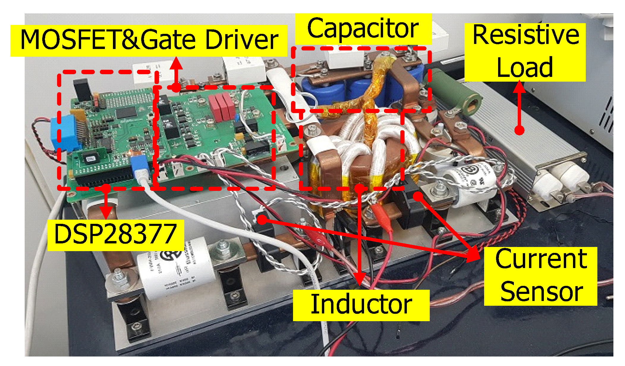
5. Experimental Results

Figure 6 presents the 3-kW bi-directional DC/DC converter testbed used to verify the feasibility of the proposed solution; A Texas Instrument (TI) digital signal processor (TI DSP28377) was used for feedback control at the constant input DC voltage level $v_s=100$ V (provided by the DC power supply) with the sampling and PWM periods of $0.1$ ms. The inductor and output capacitor values were identified $L=1$ mH and $C=700$ µF. To consider the model-plant mismatch causing the lumped disturbances, their nominal values $L_0$ = 0.75 L and $C_0$ = 1.35 C were used for the implementation of the control law. A resistive load of $R_L=20\mathsf{\Omega }$ was initially connected to the output port to implement the load of the converter.

The inner and outer loops controlled by the proposed controller were tuned as: (inner loop) $f_{cc}=5$ Hz (${\lambda }_{cc}=2\pi f_{cc}=31.4$ rad/s), ${\gamma }_{cc}=1000$, ${\sigma }_{cc}=5000/{\gamma }_{cc}$, $k_{cc}=5000$, $b_{d,L}=0.1$, $l_{i_c}=1200$, (outer loop) $f_{vc}=5$ Hz (${\lambda }_{vc}=2\pi f_{vc}=31.4$ rad/s), and $b_{d,v}=3$.

A comparative investigation was conducted by replacing the proposed controller with a conventional PI controller reinforced by a DOB and the active damping term: (control) $u=\frac{1}{v_{s,0}}(-k_{d,L}{i}_L+L_0{\lambda }_{cc}{\tilde{i}}_c+k_{d,L}{\lambda }_{cc}{\int }_0^t{\tilde{i}}_{c}d\tau -{\widehat{d}}_L)$, (DOB) ${\dot{z}}_L=-l_{i_c}{z}_L-l_{i_c}^2{L}_0{i}_c-l_{i_c}{v}_{s,0}u$, and ${\widehat{d}}_L=z_L+l_{i_c}{L}_0{i}_c$. The design parameters are identical to those in the proposed solution.

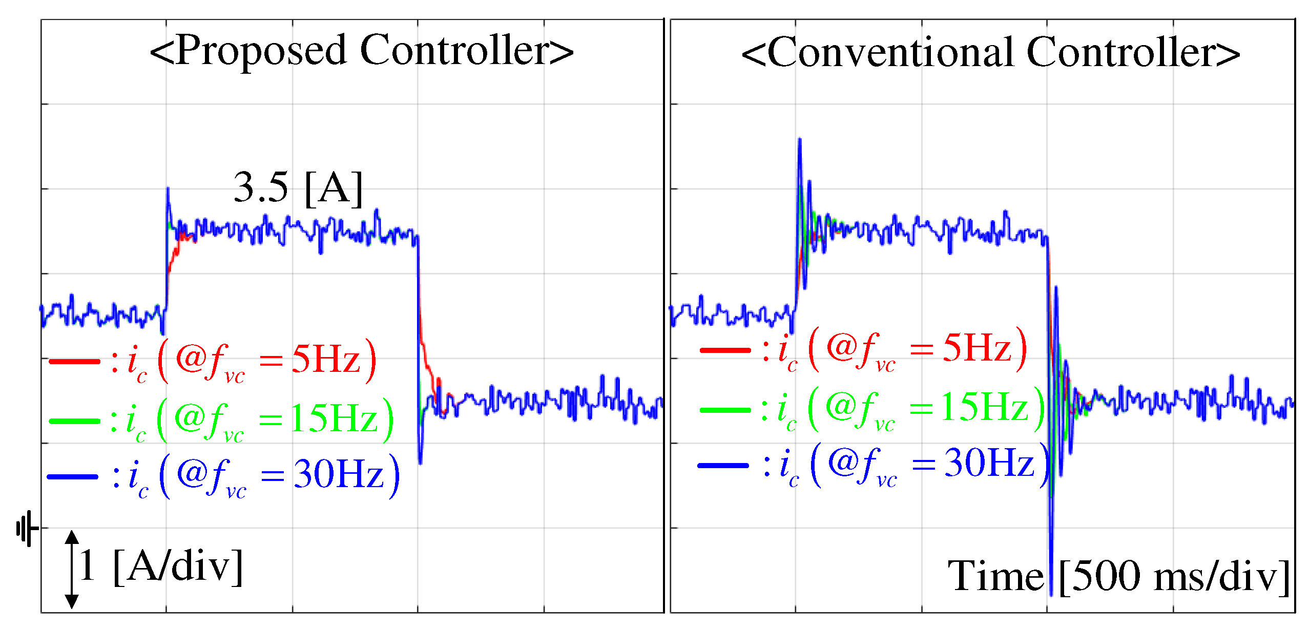
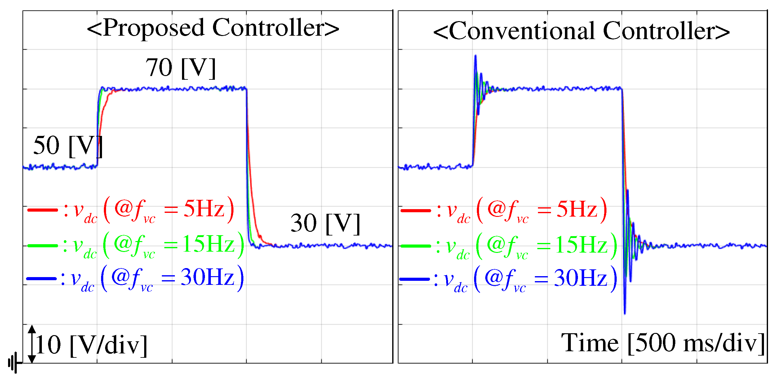
5.1. Piece-Wise Constant Reference Tracking Mode

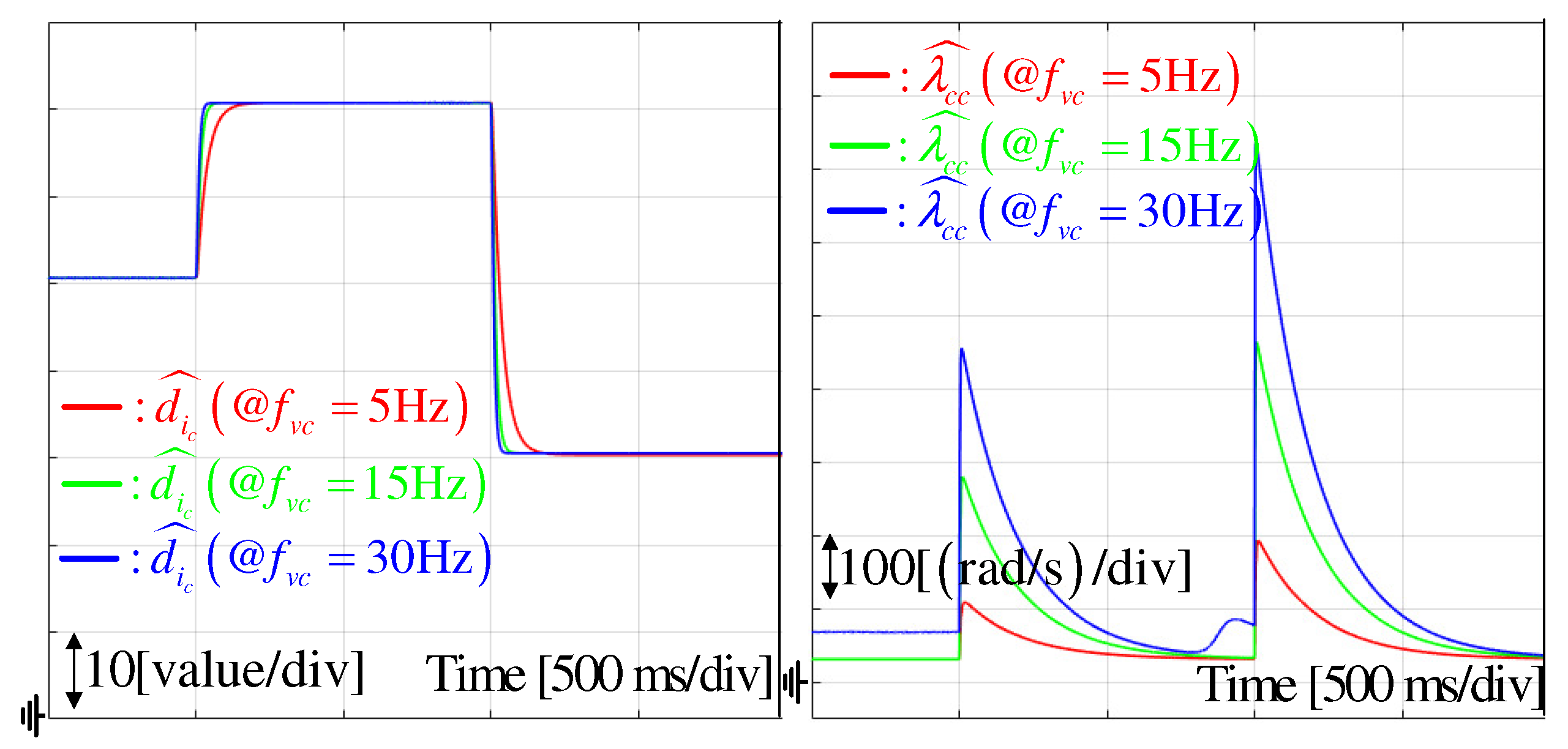
The initial output voltage reference $v_{dc,ref}=50$ V was increased and decreased to 70 and 30 V in a sequential manner with an initial resistive load $R_L=20\mathsf{\Omega }$. Figure 7 shows the controlled output voltages obtained using the proposed and conventional techniques. Unlike the conventional controller, the proposed controller successfully drives the output voltage to its reference value without any over/undershoots. Moreover, the proposed controller successfully assigns the desired tracking behavior to the resultant feedback system in accordance with the performance (5) achieved with the increased output voltage cut-off frequencies $f_{vc}=5$, 15, and 30 Hz. 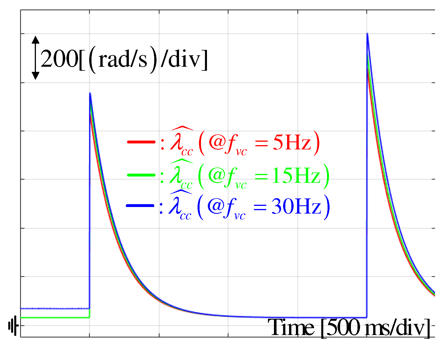The exponential convergence (6) (proven by Theorem 3) and nature of the current-loop cut-off frequency boosting (resulting in ${\dot{V}}_c\le -{\alpha }_c{V}_c<0$ proven by Theorem 2) provide this advantage without the drawback of performance degradation. 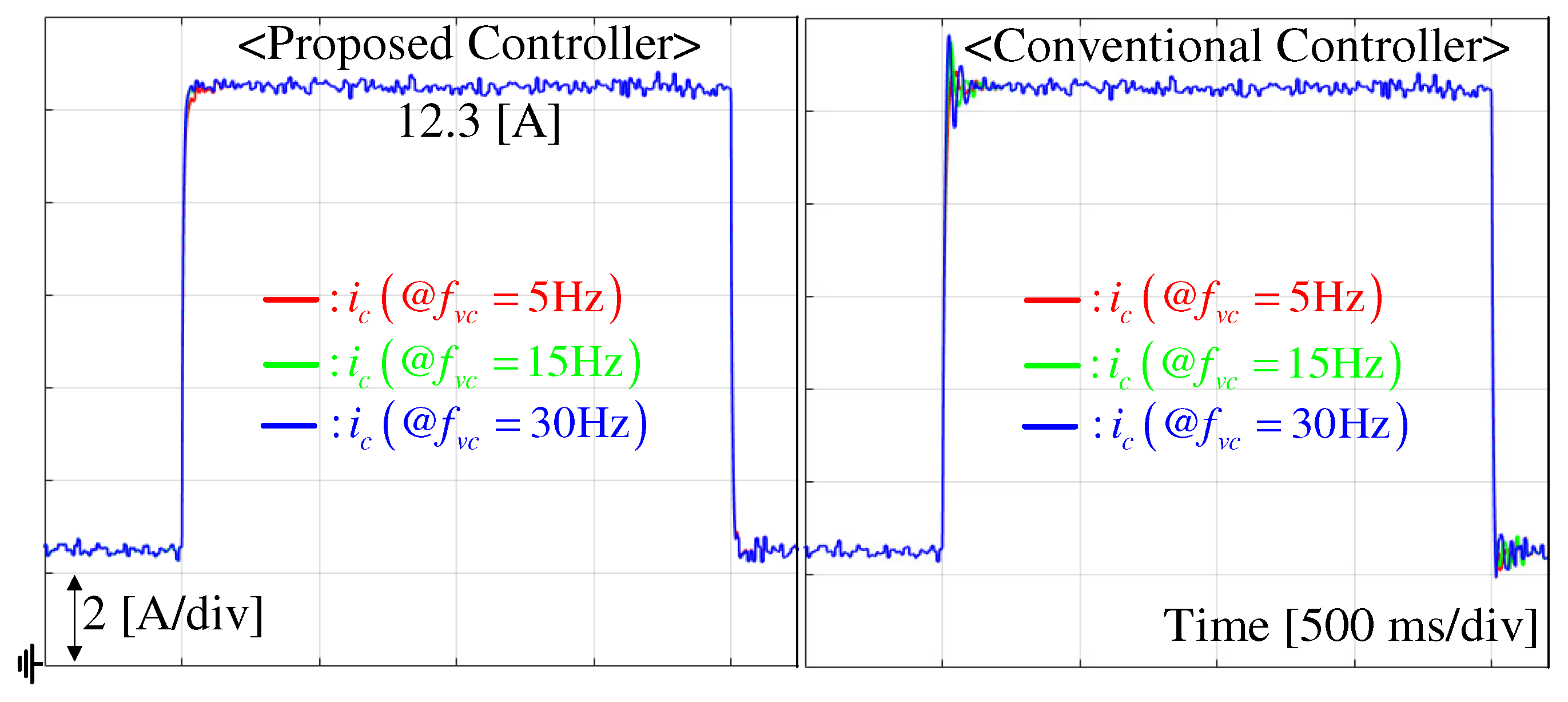Notably, the advantage originates from the dynamic current cut-off frequency (boosting and restoration) presented on the right side of Figure 8. As expected, the proposed controller removes the unnecessary current oscillation and reduces the current overshoot level, as shown in Figure 9. The DOB responses are presented on the left side of Figure 8.

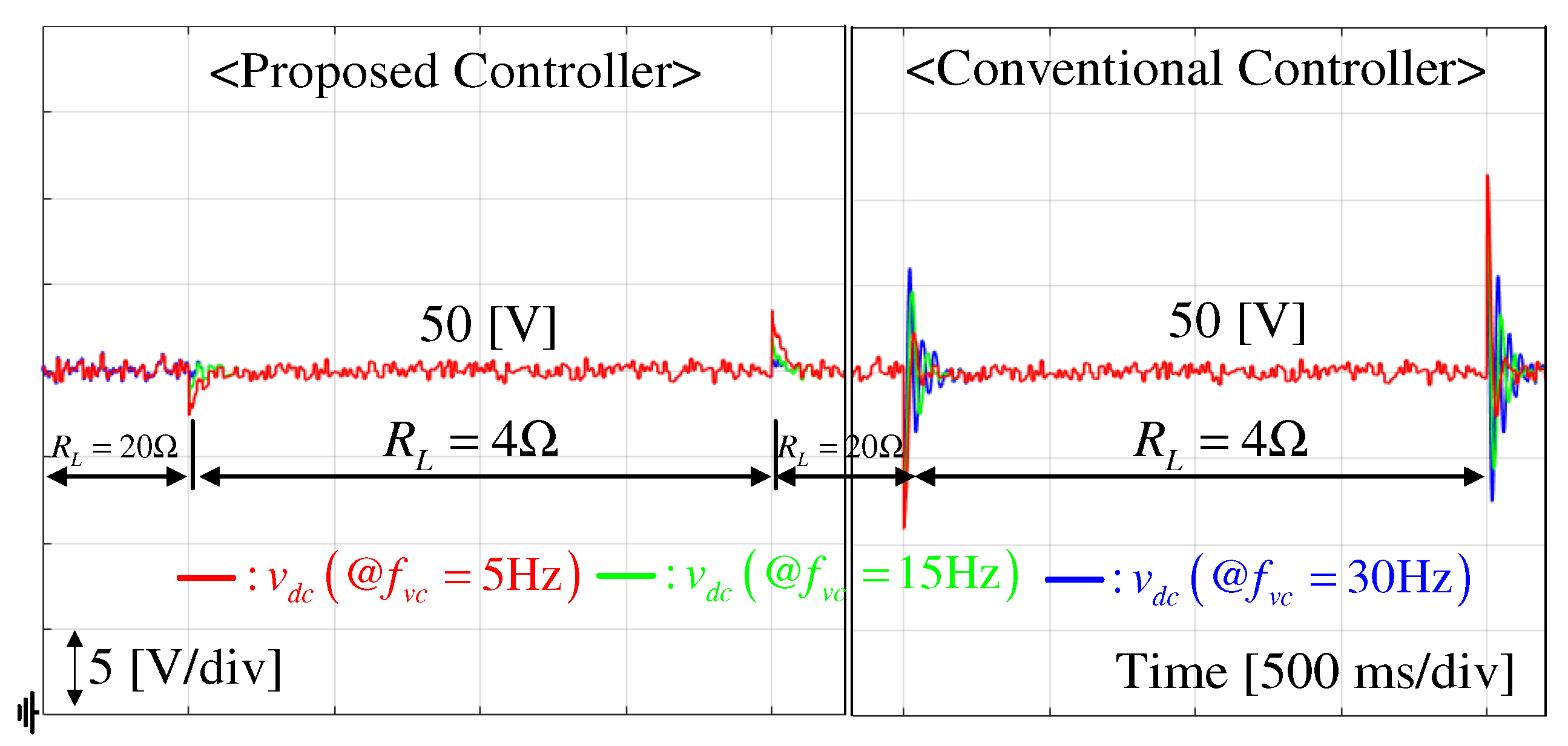
5.2. Constant Reference Regulation Mode

5.2.1. Transient Performance Comparison

This stage demonstrates the constant reference regulation performance at the output voltage level of 50 V with an abrupt variation in the resistive load (decreasing to $R_L=4$ $\mathsf{\Omega }$ and restoring to $R_L=20$ $\mathsf{\Omega }$). The three output voltage cut-off frequencies $f_{vc}=5$, 15, and 30 Hz were applied to clarify the advantages of the proposed controller. As shown in Figure 10, the proposed controller can effectively attenuate the over/undershoot level and the performance deviations caused by the variation of the operating conditions. The removal of the current oscillation and overshoot can also be observed in Figure 11. As intended, the collaboration of two beneficial properties, namely, the cut-off frequency magnification (Lemma 1) and exponential current convergence (Theorem 1), resulted in this beneficial feature.

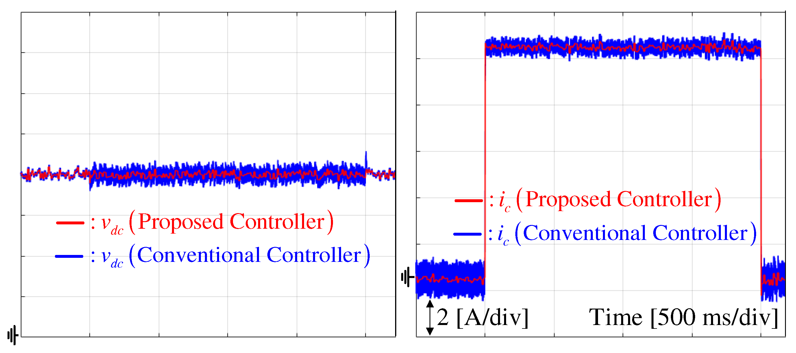
5.2.2. Steady-State Behavior Comparison

This stage shows the current ripple reduction effect from the proposed current cut-off frequency auto-tuner at the same operating mode of the previous subsection, except for the constant cut-off frequency for the conventional DOB-based controller. To secure the improved closed-loop performance, the current cut-off frequency (fixed) for the conventional controller was increased from its initial setting $f_{cc}=5$ to 190 Hz that is equal to the peak value of the dynamic current cut-off frequency shown in Figure 12. As presented in Figure 13, the increased current cut-off frequency successfully attenuates the over/undershoots but it involves the current ripple magnification in the steady-state operation unlike the proposed controller. The dynamic current cut-off frequency behavior shown in Figure 12 offers this beneficial current ripple reduction characteristics increasing the power efficiency for a long term operation.

5.3. Discussion

5.3.1. Computational Time

The proposed controller comprising novel subsystems, such as the auto-tuner (10) and target dynamics (9), requires additional computational time compared with that of the conventional DOB controller used for the comparison study in this section. To confirm this, the execution time for these two controllers was determined for 3000 randomly generated 3000 reference signals using the DSP28377, based on the pulse length for the whole control algorithm code. The proposed and conventional DOB controllers elapsed $33.87$ and 30.75 µs, respectively, on an average. This implies that only additional $10\%$ of computational time is required for the proposed controller compared with that of the conventional DOB controller. On the basis of these comparisons for the performance and computational complexity, the proposed controller can be considered as an alternative to previous solutions without the need for additional hardware (compared with the full-state feedback results) under the use of 32-bit DSPs.

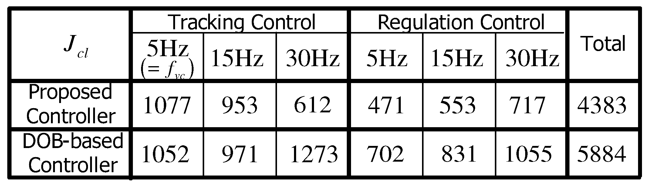
5.3.2. Quantitative Comparison

Section 5.1 and Section 5.2 present the qualitative differences between the closed-loop responses. To clarify the performance improvement, the metric function is adopted regarding the output voltage error integration during the operation time (for both the tracking and regulation modes), which is given by $J_{cl}:=\sqrt{{\int }_0^{\infty }{|v_{dc,ref}-v_{dc}|}^{2}dt}$. The table in Figure 14 presents the comparison result with the proposed technique achieving a $34\%$ performance enhancement owing to its improved controller structure and novel inner loop subsystems (leading to the beneficial closed-loop properties in Section 4).

6. Conclusions

This study developed a cascade-type output voltage controller governed by the dynamic current cut-off frequency from a real-time auto-tuner. The outer loop employs an active damping term to suppress the disturbance level and invokes closed-loop order reduction with pole-zero cancellation, which is provided by the particular design of the feedback gain structure. A significant admissible output voltage cut-off frequency range expansion caused by the dynamic current cut-off frequency behavior was observed in the experimental investigation. There are two future research branches: first, the expansions of the proposed solution to the multi-phase converter and multi-converter power synchronization applications and, second, the development of a systematic tuning factor design criteria through an optimization problem formulation subject to the linear/bi-linear matrix inequality(LMI/BMI) constraints.