PMSM Torque-Speed-Efficiency Map Evaluation from Parameter Estimation Based on the Stand Still Test

Abstract

During the last decades, a wide variety of methods to estimate permanent magnet synchronous motor (PMSM) performance have been developed. These methodologies have several advantages over conventional procedures, saving time and economic costs. This paper presents a new methodology to estimate the PMSM torque-speed-efficiency map based on the blocked rotor test using a single-phase voltage source. The methodology identifies the stator flux linkage depending on the current magnitude and angle while providing a detailed estimation of the iron losses. The torque-speed-efficiency map provides detailed information of the motor efficiency along its operating region, including the nominal conditions and the maximum power envelope. The proposed methodology does not require knowing the geometry of the machine to perform any load test, and it also avoids using expensive measurement devices and a complex experimental setup. Moreover, the proposed method allows the PMSM performance to be reproduced by applying different control strategies, which is useful when testing different drives. The method does not require the application of any optimization algorithm, thus simplifying and speeding up the process to determine the performance. Experimental validation is carried out by comparing motor performances obtained through the proposed method with those obtained by means of a conventional experimental method and against finite element analysis (FEA).

1. Introduction

Performance evaluation of permanent magnet synchronous machines PMSM is an active research field because it enables reproduction of the machine performance, reducing time, saving economic resources and allowing for the reproduction of different scenarios [1]. Traditional testing methodologies require a great deal of time and effort to prepare the experimental setup and to test different operating conditions. For instance, conventional tests include the non-load test, torque test, load test, loss test, thermal test and inductance test, among others. Data synchronization and the selection of the instrumentation in order to adapt the measurements to the specific application adds complexity to the problem.

Some standardized tests to measure PMSMs parameters to characterize its performance were proposed, as the standstill frequency response (SSFR) [2,3,4]. In [5], a test based on generating sinusoidal signals by using a voltage-source inverter was proposed. The IEEE 115-2019 standard [6] for synchronous machines performance identification considers different testing methods; nevertheless, most of them are not applicable to PMSMs. Some testing methodologies for PMSMs were proposed in the literature. For instance, [7] proposes an indirect testing methodology for the mechanical characteristic of the multiunit PMSM under no-load conditions. Other studies focus on analyzing the PMSM losses by indirect testing as [8] or [9], which develops a practical testing solution to optimally design the stator harmonic currents to minimize the torque ripple using speed harmonics. Other studies focus on estimating the PMSM parameters to reproduce the motor performance using mathematical models together with voltages, currents and rotor speed [10]. A wide range of methodologies was proposed in the literature, and they are categorized into online and offline parameter identification [1].

Online parameter identification operates in real time while the motor is running under normal conditions. There are three main categories: online numerical methods [11,12,13], online artificial intelligence (AI) methods [14,15] and observer-based [16,17,18,19] methods. Some recent studies within this category estimate the motor parameters by considering the disturbance voltage [20]. Other studies [21] develop a sensorless speed tracking approach for PMSMs. Other studies focus on identifying a specific parameter. In [22], the rotor position is estimated at low-speed regimes based on an active flux sensorless control. Further developments were presented in [23] by identifying the stator winding resistance, permanent magnet flux linkages. More recent studies focus on improving sensorless controls by applying parameter identification approaches. Following this example, [24] develops a sensorless online parameter estimation method to detect the load current when operating at low-speed regimes, which is mainly affected by the estimation error of the rotor position.

Offline parameter identification methodologies are designed to obtain data from specific tests, which require disconnecting the motor from the normal operation and performing different experiments to extract data. Offline methodologies are divided into three main categories, frequency-domain methods [3,25], time-domain methods [10,26] and finite element methods [27]. Earlier studies in offline methods, as in [28], show an experimental test procedure to identify the magnetic parameters in a lumped model by evaluating the flux linkages from voltage acquisitions. Other improvements are found in [29], where the parameters of the magnetic model are identified from tests. Further developments are presented in [30], where the cross-coupling effect and magnetic saturation are included in the model. Other studies focus on finding the rotor position from the current waveforms [31] without using a position sensor [32].

This paper presents a novel performance estimation methodology for PMSMs based on the blocked rotor test using a single-phase voltage source. The PMSM performance is evaluated by calculating the torque-speed-efficiency map, which provides information on the motor efficiency along the whole operating region, including the nominal conditions and the maximum power envelope. The methodology identifies the stator flux linkage as a function of the current magnitude and angle while providing a detailed estimation of iron losses over current and main frequency. The methodology does not require knowing the geometry of the PMSM. This method avoids the use of expensive measurement devices and does not require a complex experimental setup. Moreover, as the parameters are identified as a function of the load conditions, this method allows for the reproduction of the PMSM performance by applying different control strategies using a d-q electrical model. The method does not require any optimization algorithm, thus simplifying and speeding up the process to reproduce the performance. The method is validated experimentally by comparing PMSM torque-speed-efficiency maps and electromagnetic parameters using finite element analysis (FEA) and direct operation experimental tests.

This research work is structured in different sections. Section 2 details the permanent magnet synchronous motor and water pump system (PMSM-WP) testing and performance analysis methodology to evaluate the motor parameters and reproduce the motor performance. Section 3 exposes the results and validation analysis. Finally, Section 4 concludes the paper.

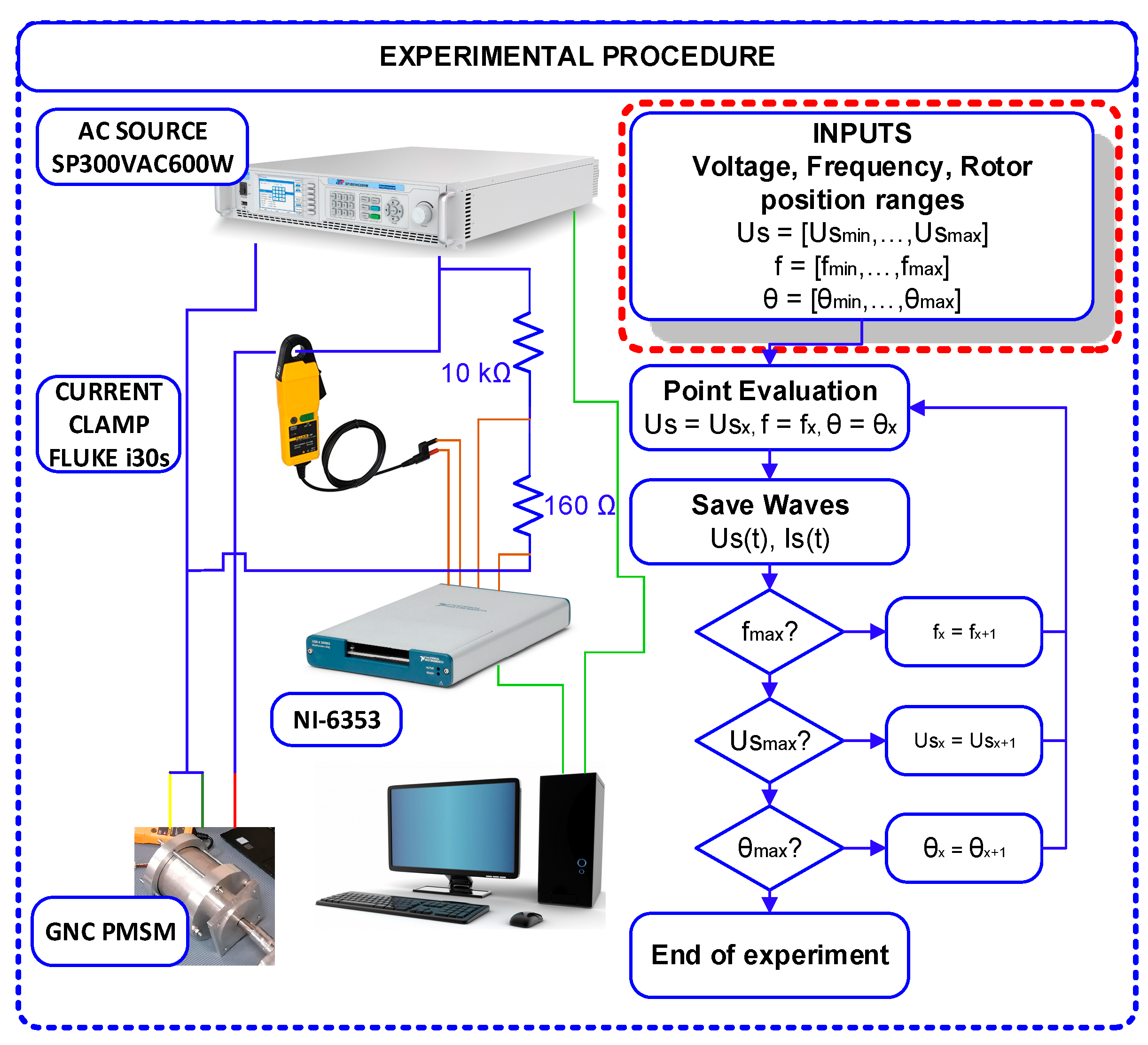
2. PMSM Blocked Rotor Test and Performance Analysis Methodology

This section introduces the testing procedure under blocked rotor conditions and the PMSM performance analysis methodology proposed in this work. First, a series of experiments were performed in order to acquire electrical data. The experimental setup and experimental procedure are exposed in Figure 1. The experimental test procedure consists of connecting a single-phase voltage source to a three-phase PMSM. The positive terminal is connected to the reference phase or phase “a” for convention, whereas the negative terminal is connected to the other two remaining phases. This configuration allows for the reproduction of the space vector current when the current is at its maximum value. The magnitudes to be acquired are the instantaneous values of the voltage and current when applying different electrical frequencies and RMS voltages with the single-phase voltage source. The procedure includes three main parameters, i.e., frequency, RMS voltage and rotor angle. The objective is to acquire the electrical magnitudes for each combination for a posterior analysis using the electrical circuit shown in Figure 2a.

Once the time-varying magnitudes are acquired, these are post-processed in order to identify the parameters required to reproduce the motor performance.

Two electrical models are required to extract the PMSM parameters (Figure 2a) and to reproduce the PMSM performance (Figure 2b). Figure 2 shows the parameter estimation electrical model and the d-q electrical model. The inductance is split into leakage and linkage components.

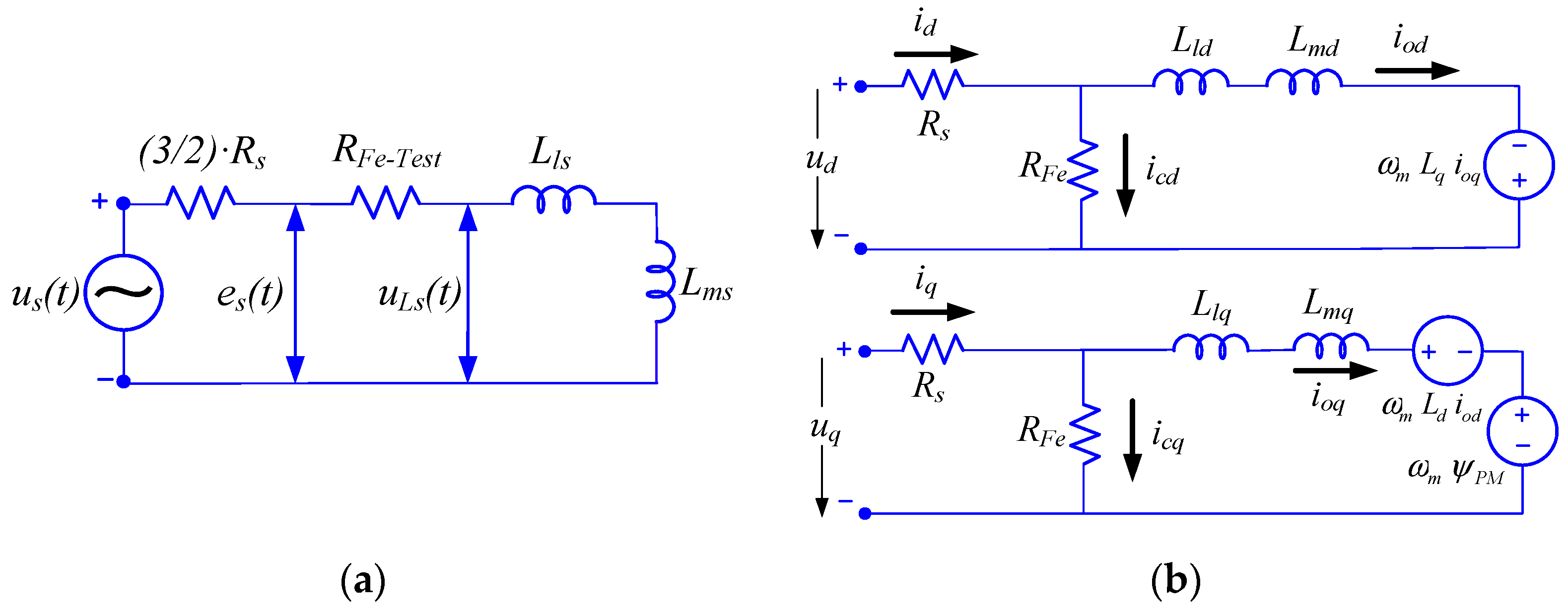
2.1. Parameter Estimation Electrical Model

To carry out the parameter estimation process, as shown in Figure 2, a series resistor to represent iron losses is required. The main magnitudes to be identified are the iron losses and the stator inductance, which are required in the d-q electrical model. First, a digital low-pass filter is applied in order to remove the noise effect on the identification. It is a first-order low-pass filter. The filter has a stopband attenuation of 60 dB. The cut-off frequency is selected to the 11th electrical harmonic frequency. Next, for each voltage-frequency-rotor angle combination, the voltage drop due to the iron losses and inductance is calculated as

$$e_s\left(t\right)=u_s\left(t\right)-i_s\left(t\right)\cdot \frac{m}{2}$$

(1)

The instantaneous iron power is computed from e_s(t) and i_s(t) as

$$P_{si}\left(t\right)=e_s\left(t\right)·i_{´s}\left(t\right)$$

(2)

Next, the mean power consumed by the iron resistor model is calculated as

$${\overline{P}}_{Fe-Test}=mean\left(P_{si}\left(t\right)\right)$$

(3)

The equivalent series resistor in Figure 2a modeling the iron losses is computed as

$$R_{Fe-Test}=\frac{{\overline{P}}_{Fe-Test}}{{\left(i_{s-RMS}\right)}^2}$$

(4)

Now, assuming the iron losses resistor constant, the instantaneous iron losses are computed as

$$P_{Fe-Test}\left(t\right)=R_{Fe-Test}·{\left(i_s\left(t\right)\right)}^2$$

(5)

Therefore, the instantaneous power in the inductor, whose mean value is zero, is calculated as

$$P_{Ls}\left(t\right)=P_{si}\left(t\right)-P_{Fe-Test}\left(t\right)$$

(6)

The voltage drop across the inductor is calculated as

$$u_{Ls}\left(t\right)=e_s\left(t\right)-R_{Fe-Test}\cdot i_s\left(t\right)$$

(7)

With the temporal expression of voltage across the inductor and current available, the differential equation in (8) is solved, and L_s(t) is obtained.

$$u_{Ls}\left(t\right)=L_s\left(t\right)\cdot \frac{d{i}_s\left(t\right)}{dt}+i_s\left(t\right)\cdot \frac{d{L}_s\left(t\right)}{dt}$$

(8)

In this case, L_s (t) = L_ls (t) + L_ms (t) is defined as the sum of the leakage and linkage inductances, respectively.

Once the instantaneous values of the linkage and leakage inductors are found, the characteristic value of the inductance corresponds to that when the maximum current value occurs, i.e., when the current space vector is in its maximum values for the specific tested rotor position.

The numerical values of L_s(t) become unstable when reaching the current reaches its maximum because the term di_s(t)/dt is zero. For this reason, the values to be considered are those close to the maximum, which in this case is taken three degrees before and after the maximum of the current. Within the electrical period, the maximum and minimum current values are reached at 90° and 270°, respectively, the angles to select the inductance are 87° and 93°. These values are averaged to have a unique value for each maximum peak. Then, all values gathered at each peak are averaged to obtain a unique inductance for each studied case, whose value is L_s(i_d,i_q). Next, the values obtained from the parameter estimation process are used to calculate the differential stator flux linkage, i.e., the flux linkage generated by the stator windings as ΔΨ_s(i_d,i_q) = L_s(i_d,i_q)·i_s. Then, considering the electrical angle, this flux linkage is projected along the d-q axis reference, thus obtaining the d-q fluxes generated by the stator windings. The permanent magnet flux linkage is usually found in the machine nameplate. If this magnitude is not provided, an open circuit test can be performed to obtain the first harmonic of the back electromotive force produced by the permanent magnets. Therefore, the direct axis flux linkage is obtained as the sum of the permanent magnet flux linkage and the differential flux linkage generated by the stator windings, Ψ_d = Ψ_PM + ΔΨ_s(i_d,i_q)·θ_e= Ψ_PM + L_d(i_d,i_q)·i_d. The quadrature axis flux linkage is directly the projection of the flux linkage produced by the stator windings along the q axis, Ψ_q = ΔΨ_s(i_d,i_q)·sin(θ_e) = L_q(i_d,i_q)·i_q. The d-q inductances of the electric model are defined in Figure 2b. As already mentioned, the inductance obtained through the parameter estimation process considers the magnetizing and leakage inductances, so the d-q inductances derived from this process consider the leakage and linkage components.

Finally, following the same criterion, the temporal expression of power losses is a corrected sinusoidal wave. The peaks are the correspondent losses when the current space vector is at its maximum value. Figure 3 shows a specific example of the instantaneous iron losses.

As can be seen in Figure 3, the peaks are those where the current space vector is maximum. The higher peaks correspond to the space vector currents, which contribute to the permanent magnet flux. The peak values are those providing information about the losses under normal conditions.

The reason behind this approximation arises from the theory of magnetic losses, which can be deduced from the classical Bertotti equations in the time domain.

$$P_{Fe-Eddy}=\frac{\sigma \cdot h^2}{12\cdot T}\cdot {{\displaystyle \underset{0}{\overset{T}{\int }}{\displaystyle \underset{d\forall }{\int }\left(\frac{dB}{dt}\right)}}}^2\cdot d\forall \cdot dt$$

(9)

$$P_{Fe-Hyst}=\frac{K_h\cdot \rho }{T}\cdot {{\displaystyle \underset{d\forall }{\int }{B}_m}}^{\alpha }\cdot \left(1+{\displaystyle \sum _{i=1}^n\frac{\beta }{B_m}\cdot \left(\Delta B_i\right)}\right)\cdot d\forall$$

(10)

$$P_{Fe-Excess}=\frac{K_{exc}\cdot \rho }{T}\cdot {{\displaystyle \underset{0}{\overset{T}{\int }}{\displaystyle \underset{d\forall }{\int }\left(\left|\frac{dB}{dt}\right|\right)}}}^{1.5}\cdot d\forall \cdot dt$$

(11)

Considering Equations (9)–(11), the losses are computed based on the magnetic flux density variation in a differential time and its absolute magnitude. It is noted that B is the magnetic flux density, σ is the electrical conductivity of iron, h is the lamination’s thickness, dⱯ is the differential volume, T is the time period, K_{h is} the hysteresis constant, dt is the differential time, ρ is the iron laminations density, α and β are the hysteresis exponents, and K_{exc is} the excess constant.

For a small differential time dt, the space vector current is changed by a differential electrical angle dθ when the motor is operating under normal conditions. Thus, the so-called space–time conversion can be applied.

$$\left(\frac{dB}{d{\theta }_e}\right)=\left(\frac{dB}{dt}\right)\cdot \left(\frac{dt}{d{\theta }_e}\right)\to \left(\frac{dB}{dt}\right)=\left(\frac{dB}{d{\theta }_e}\right)\cdot {\omega }_e$$

(12)

The losses derived from this process consider the total magnetic losses because the space–time conversion was applied with a specific current space vector, thus considering the contribution of the three phases.

Algorithm 1 summarizes the parameter estimation process.

Algorithm 1. Parameter analysis extraction algorithm.

1: Take $u_{´s}\left(t\right)$ and $i_{´s}\left(t\right)$ for each voltage, frequency and rotor position combination.

2: Apply a digital low pass filter.

3: Compute iron losses and inductance voltage drop: $e_s\left(t\right)=u_s\left(t\right)-i_s\left(t\right)\cdot R_s\cdot \frac{m}{2}$

4: Compute instantaneous power: $P_{si}\left(t\right)=e_s\left(t\right)\cdot i_s\left(t\right)$

5: Compute mean iron losses power: ${\overline{P}}_{Fe}=mean\left(P_{si}\left(t\right)\right)$

6: Compute equivalent iron losses resistor: $R_{Fe}=P_{Fe-mean}/i_{s-RMS}{}^2$

7: Compute instantaneous iron losses: $P_{Fe}\left(t\right)=i_s{\left(t\right)}^2\cdot R_{Fe}$

8: Compute instantaneous reactive power: $P_{Ls}\left(t\right)=P_{ti}\left(t\right)-P_{Fe}\left(t\right)$

9: Compute linkage + leakage induction voltage: $U_{L_s}\left(t\right)=E_s\left(t\right)-I_{s-f}\left(t\right)\cdot R_{Fe}$

11: Linkage + leakage inductance calculation: $E_s\left(t\right)=L_s\left(t\right)\cdot \frac{d{I}_{s-f}}{dt}+I_{s-f}\left(t\right)\cdot \frac{d{L}_s}{dt}$ → $L_s\left(t\right)$

12: Stator inductance as a function of the d-q currents: $L_s\left(t\right)$ → $L_s\left(i_d,i_q\right)$

13: Compute the flux linkage gradient using the stator inductance $L_s\left(i_d,i_q\right)$: $\Delta {\Psi }_s=L_s\left(i_d,i_q\right)\cdot i_s\left(i_d,i_q\right)$

14: Determination of the d-q flux linkage: $\{\begin{array}{l}{\Psi }_d={\Psi }_{PM}+\Delta {\Psi }_s\cdot \cos \left({\theta }_e\right)={\Psi }_{PM}+L_d\left(i_d,i_q\right)\cdot i_d\\ {\Psi }_q=\Delta {\Psi }_s\cdot \sin \left({\theta }_e\right)=L_q\left(i_d,i_q\right)\cdot i_q\end{array}$

15: Selection of representative inductance for the space vector current: $\{\begin{array}{l}{\Psi }_d={\Psi }_{PM}+\Delta {\Psi }_s\cdot \cos \left({\theta }_e\right)={\Psi }_{PM}+L_d\left(i_d,i_q\right)\cdot i_d\\ {\Psi }_q=\Delta {\Psi }_s\cdot \sin \left({\theta }_e\right)=L_q\left(i_d,i_q\right)\cdot i_q\end{array}$ → $L_d\left(i_d,i_q\right)$$, L_q\left(i_d,i_q\right)$

16: Selection of iron losses for real operating conditions: $P_{Fe}\left(i_d,i_q,f\right)$

2.2. d-q Electrical Model for Performance Analysis

Once the parameters are estimated, i.e., the d-q inductances, copper losses and iron losses, the quasi-static d-q electrical model equations are used [33]. The main advantage of using this model is the possibility of testing multiple control strategies, which is a huge advantage over other models [34].

As a first step, by considering the circuit introduced in Figure 2b, the od and oq currents are discretized within the motoring quadrant. Next, a series of computations are performed in order to reproduce the motor performance. The process is as follows.

First, according to the od and oq current values, the values of inductance identified during the test are extracted.

$$\{\begin{array}{l}{L}_d\left(i_{od},i_{oq}\right)\\ L_q\left(i_{od},i_{oq}\right)\end{array}$$

(13)

By considering the d-q currents and inductances calculated in the previous step, the d-q flux linkages are calculated. The permanent magnet flux linkage is a nameplate parameter. If this magnitude is not provided, an open circuit test should be performed in order to obtain the first harmonic of the back electromotive force produced by the permanent magnets.

$$\{\begin{array}{l}{\Psi }_d={\Psi }_{PM}+L_d·i_{od}\\ {\Psi }_q=L_q·i_{oq}\end{array}$$

(14)

The torque can be computed at this stage as

$$T=\frac{m}{2}\cdot p\cdot \left({\Psi }_{PM}·i_{oq}-\left(L_q-L_d\right)\cdot i_{od}\cdot i_{oq}\right)$$

(15)

From the od and oq current values, the iron losses are extracted:

$$P_{Fe}\left(i_{od},i_{oq},{\omega }_m\right)$$

(16)

The back electromotive force is as

$$\{\begin{array}{l}{u}_{od}=-{\omega }_e\cdot L_q\cdot i_{oq}=-{\Psi }_q\cdot {\omega }_e\\ u_{oq}={\omega }_e\cdot \left(L_d\cdot i_{od}+{\Psi }_{PM}\right)={\Psi }_d\cdot {\omega }_e\end{array}$$

(17)

As the magnetic losses are known, the parallel resistance is calculated as

$$R_{Fe}=m\cdot \left(u_{od}{}^2+u_{oq}{}^2\right)/\left(2\cdot P_{Fe}\right)$$

(18)

The currents i_cd and i_cq are calculated from the iron resistance

$$\{\begin{array}{l}{i}_{cd}=u_{od}/R_{Fe}\\ i_{cq}=u_{oq}/R_{Fe}\end{array}$$

(19)

The total current i_d and i_q are calculated. The voltage equations are as follows:

$$\{\begin{array}{l}{u}_d=R_s\cdot i_d+L_d\cdot \frac{d}{dt}\cdot i_{od}-{\omega }_e\cdot L_q\cdot i_{oq}\\ u_q=R_s\cdot i_q+L_q\cdot \frac{d}{dt}\cdot i_{oq}+{\omega }_e\cdot L_d\cdot i_{od}+{\omega }_e\cdot {\Psi }_{PM}\end{array}$$

(20)

Finally, once the data of the discretized current values and angular speeds are available, the points are chosen depending on the control algorithm selected.

Algorithm 2 details the d-q electrical model computation procedure applied to extract the torque-speed-efficiency maps from the data estimated from the experiments.

Algorithm 2. (d-q) electrical model computation procedure.

1: od and oq current discretization.

2: d-q inductances values: $\{\begin{array}{l}{L}_d\left(i_{od},i_{oq}\right)\\ L_q\left(i_{od},i_{oq}\right)\end{array}$

3: Flux linkage calculation: $\{\begin{array}{l}{\Psi }_d={\Psi }_{PM}+L_d\left(i_{od},i_{oq}\right)·i_{od}\\ {\Psi }_q=L_q\left(i_{od},i_{oq}\right)·i_{oq}\end{array}$

4: Torque computation: $T=\frac{m}{2}\cdot p\cdot \left({\Psi }_{PM}·i_{oq}-\left(L_q\left(i_{od},i_{oq}\right)-L_d\left(i_{od},i_{oq}\right)\right)\cdot i_{od}\cdot i_{oq}\right)$

5: Iron losses extraction: $P_{Fe}\left(i_{od},i_{oq},{\omega }_m\right)$

6: Back electromotive force: $\{\begin{array}{l}{u}_{od}=-{\omega }_e\cdot L_q\left(i_{od},i_{oq}\right)\cdot i_{oq}=-{\Psi }_q\cdot {\omega }_e\\ u_{oq}={\omega }_e\cdot \left(L_d\left(i_{od},i_{oq}\right)\cdot i_{od}+{\Psi }_{PM}\right)={\Psi }_d\cdot {\omega }_e\end{array}$

7: Iron resistance loss: $R_{Fe}=m\cdot \left(u_{od}{}^2+u_{oq}{}^2\right)/\left(2\cdot P_{Fe}\right)$

8: Iron resistance currents cd/cq: $\{\begin{array}{l}{i}_{cd}=u_{od}/R_{Fe}\\ i_{cq}=u_{oq}/R_{Fe}\end{array}$

9: Voltage equations: $\{\begin{array}{l}{u}_d=R_s\cdot i_d+L_d\left(i_{od},i_{oq}\right)\cdot \frac{d}{dt}\cdot i_{od}-{\omega }_e\cdot L_q\left(i_{od},i_{oq}\right)\cdot i_{oq}\\ u_q=R_s\cdot i_q+L_q\left(i_{od},i_{oq}\right)\cdot \frac{d}{dt}\cdot i_{oq}+{\omega }_e\cdot L_d\left(i_{od},i_{oq}\right)\cdot i_{od}+{\omega }_e\cdot {\Psi }_{PM}\end{array}$

10: Selection of the magnitudes from control strategy.

3. Results

This section describes the evaluation of the performance of a real PMSM by applying the methodology proposed in this paper. This motor was designed and verified in previous work [35], whose characteristics are shown in

Table 1. PMSM Characteristics.

Characteristics	Value
Number of phases	3
Nominal power [W]	585
Nominal voltage [VRMS]	200
Nominal current [IRMS]	2
Nominal torque [N·m]	1.24
Nominal speed [rpm]	4501
Nominal efficiency [%]	84.2
Pairs of poles	3
Slots number	9
d-axis Inductance Ld [mH]	4.2
q-axis Inductances Lq [mH]	11.2

.

First, the PMSM is connected according to the experimental setup shown in Figure 1. As already explained in the previous section, the experimental procedure requires acquiring and discretizing the voltage, frequency and rotor angle. The discretization of these variables is detailed in

Table 2. Relevant parameters to discretize the voltage, frequency and rotor angle.

Magnitude	Minimum Value	Maximum Value	Number of Divisions
Voltage [V]	1	20	7
Frequency [Hz]	100	800	8
Rotor Angle [Deg]	0	30	4

.

The magnitudes acquired are the temporal values of the voltage and current for each rotor angle and frequency combination. Then, the process described in Section 2.1 and summarized in Algorithm 1 is applied to extract the d-q flux linkages and the iron losses. To validate the parameter estimation procedure, first, the d-q flux linkages as a function of the d-q currents are compared against the results provided by the finite element analysis (FEA).. The software used for this purpose is Altair Flux 2019^®.

Once the d-q flux linkages are validated against FEA results, Section 3.3 validates the PMSM performance using the iron losses obtained by means of the parameter estimation process. The torque-speed-efficiency map is calculated using the d-q flux linkages identified previously and following the process explained in Section 2.2 and summarized in Algorithm 2. Once the torque-speed-efficiency map is obtained using the parameter estimation process exclusively, it is compared against the torque-speed-efficiency map evaluated using the FEA model developed in Comsol Multiphysics^®, where the copper and iron losses are modeled. In addition, for a deeper analysis, the experimental torque-speed-efficiency map is obtained from a previous study [35], thus obtaining its performance in real conditions. Finally, the computational burden is estimated.

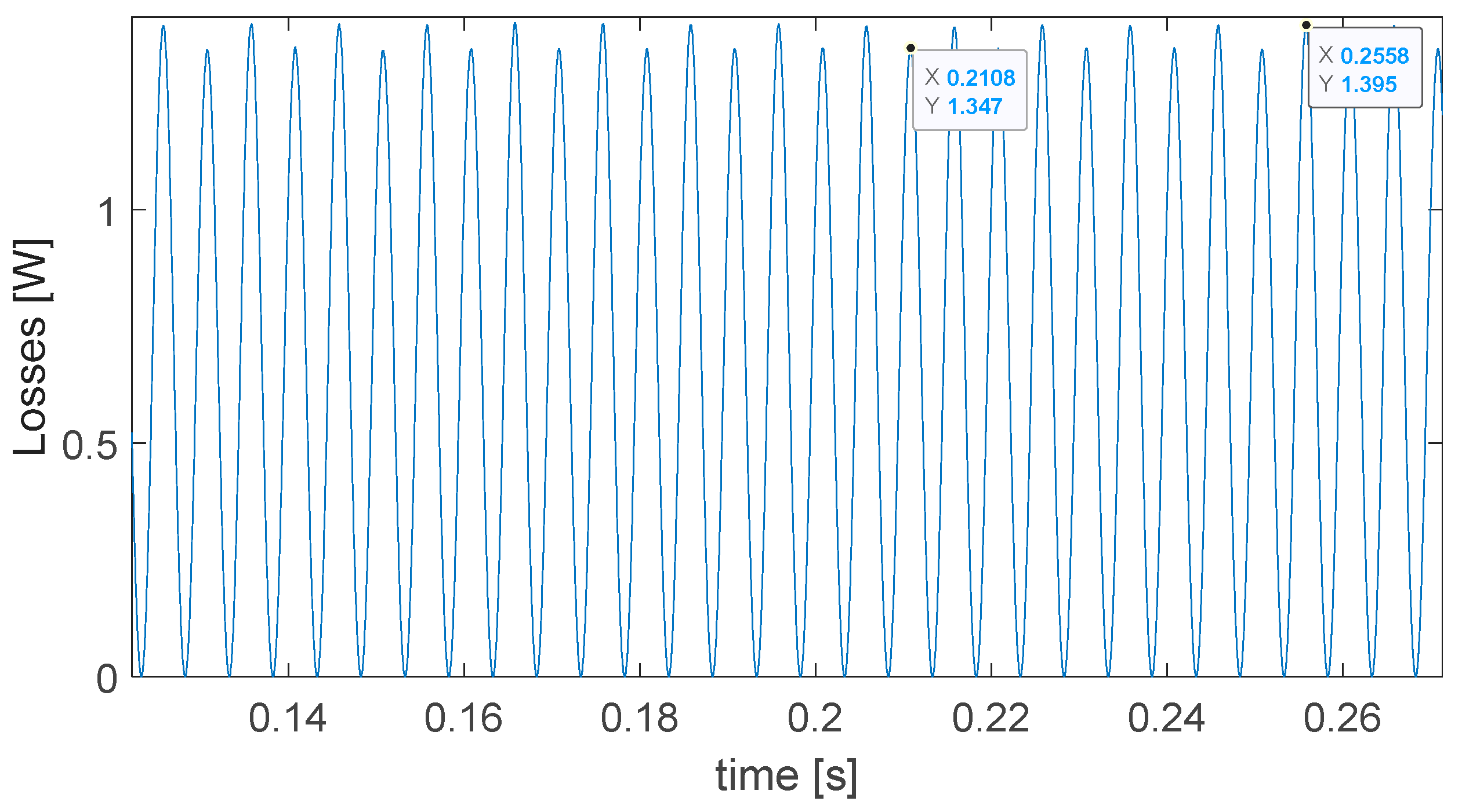
3.1. Iron Losses Estimation as a Function of the d-q Currents and Frequency

After applying the test procedure described in Section 2.1 and summarized in Algorithm 1, the inductances and iron losses are identified for each voltage, frequency and rotor angle considered. Figure 4 shows the iron losses map versus the d-q currents for each supply frequency.

As can be seen in Figure 4, and considering the electrical equivalent circuit for each test, the losses have a quadratic trend. Moreover, the lower frequency tested, i.e., 100 Hz, has more current range because the machine presents lower impedance compared to 200 Hz and 300 Hz.

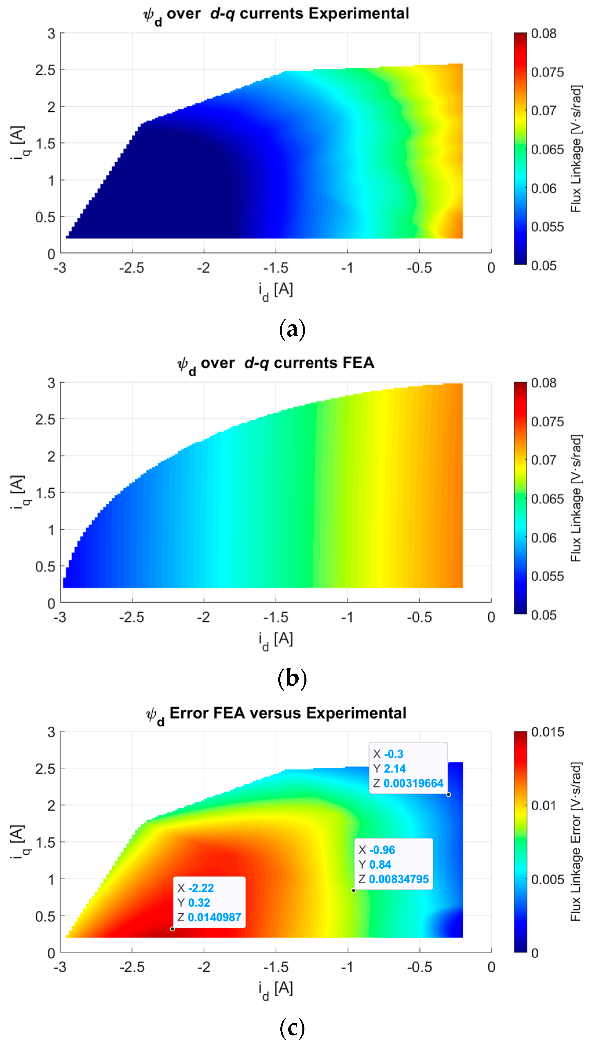
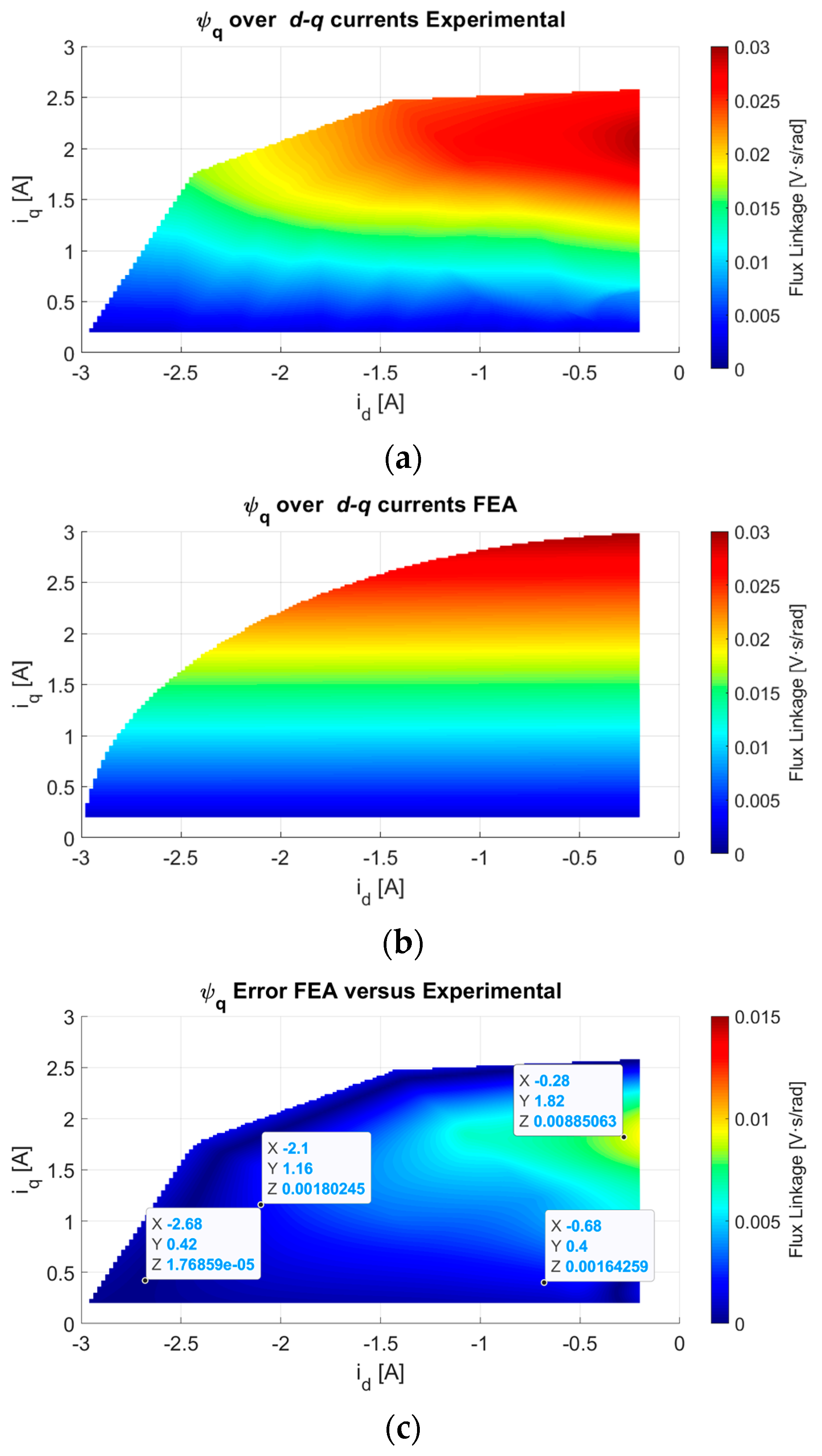
3.2. Electromagnetic Parameters Computation versus the d-q Currents

After applying the parameter estimation testing procedure, the d-q flux linkage can be computed versus the d-q currents. These magnitudes are of major importance when reproducing the PMSM performance using the d-q electrical model. In addition, the use of flux linkages simplifies the characterization.

Figure 5 and Figure 6 show the direct and quadrature axis flux linkage versus the d-q currents, respectively. Each figure compares the flux linkage obtained through the parameter estimation methodology and FEA.

As can be observed, the direct axis flux linkage values obtained by means of the parameter estimation methodology and those through FEA are similar. The distribution of this magnitude with FEA is more linear in the d axis and constant in the q axis, whereas, in the identification parameter method, it is quadratic in both axes. These differences can be due to the manufacturing tolerances of the iron lamination sheets and magnets.

In the case of the q axis flux linkage, a great similarity between the values obtained by applying the parameter estimation method and FEA is observed. In this case, a small difference in the distribution along the d-q axis is observed.

As observed in Figure 5a and Figure 7a, the parameter estimation does not cover the whole circle of possible currents due to the discretization of frequencies and rotor angles. By considering more discretized rotor angles, a smoother map can be obtained by applying the parameter estimation methodology. Moreover, the identified d axis current is larger than the values of the q axis current. This is because q axis inductance is larger, resulting in higher impedance; therefore, for the same voltage and frequency, the acquired q currents are lower.

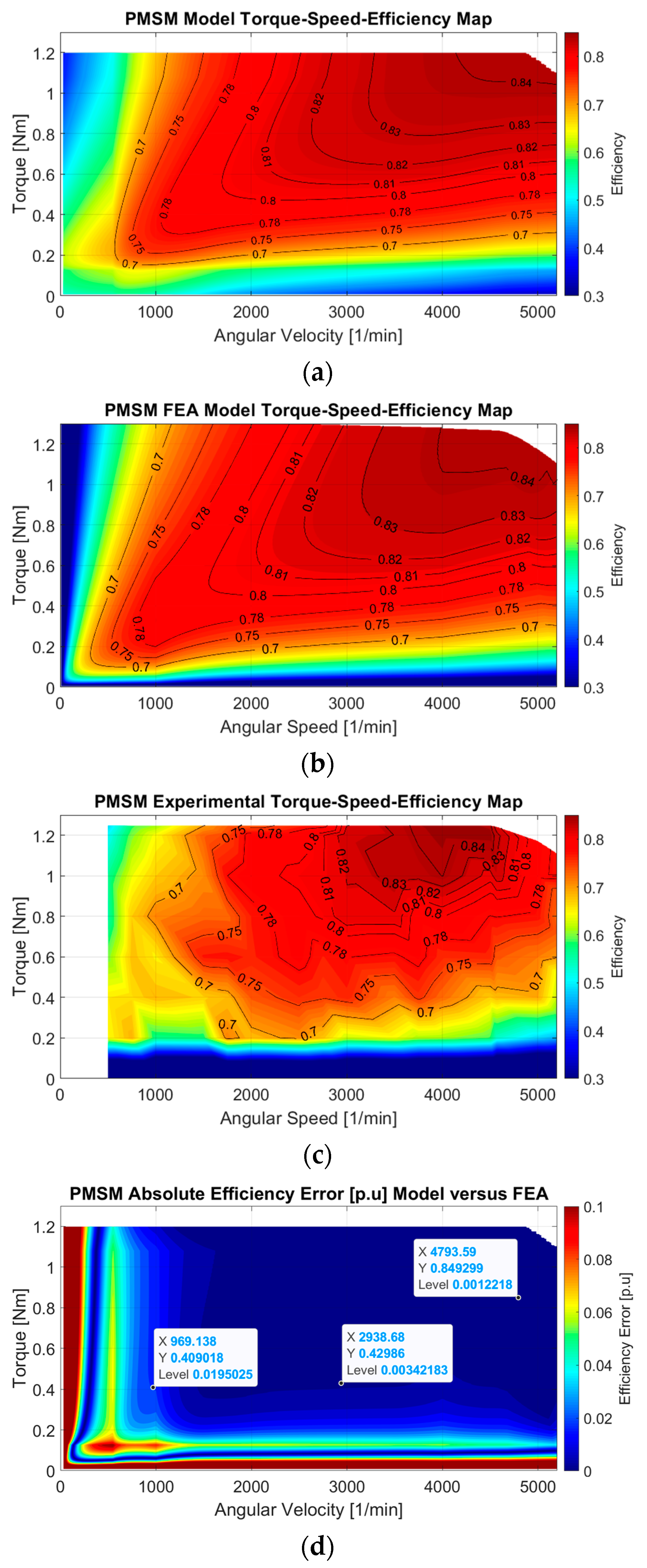
3.3. Torque-Speed-Efficiency Map Reproduction

Once the parameters are identified, the PMSM performance is reproduced. The d-q electrical model includes the winding losses and the iron lamination losses. A 90-degree current control strategy with flux weakening is considered.

Figure 7 shows the PMSM torque-speed-efficiency map found with the parameter estimation methodology (a), with FEA modeling the PMSM using Comsol Multiphysics^® (b) and obtained through experiments (c).

In Figure 7, the PMSM torque-speed-efficiency map reproduced using parameter estimation magnitudes matches with high accuracy with the performance reproduced with FEA and directly measured from experimental tests. Thus the parameter estimation magnitudes allow the PMSM real performance using the d-q electrical model with losses to be reproduced with high fidelity.

3.4. Computational Burden

The model required 1.2 s to identify the parameters and 4.1 s to reproduce the whole torque-speed-efficiency map with an Intel^® Core TM i9-7940X 3.10 GHz processor and 64 GB of RAM memory.

4. Conclusions

This paper has presented a new methodology to identify PMSM parameters to reproduce the PMSM performance by means of experiments at standstill conditions. The proposed method does not entail any previous geometry knowledge and reduces the complexity of the instrumentation required when compared with other experiments found in the technical literature. The parameters are identified as a function of the load conditions. A d-q electrical model is used, which takes into account the copper and iron losses, thus allowing for the reproduction of the load conditions. The method was validated using a commercial PMSM. The d-q flux linkages identified by the method were compared against those obtained by applying FEA simulations, showing similar values. As a second validation step, once the parameters were identified, the torque-speed-efficiency map was calculated. Then, the map was compared against FEA and experimental maps, with the three maps being very similar. Therefore, the parameter estimation method was validated not only to identify the electromagnetic parameters but also to reproduce the PMSM performance, providing detailed information on the losses. The proposed method presents a low computational burden since it is able to identify the motor parameters in only 1.2 s and reproducing the full torque-speed-efficiency map in 4.1 s.

References

1. Rafaq, M.S.; Jung, J.W. A Comprehensive Review of State-of-the-Art Parameter Estimation Techniques for Permanent Magnet Synchronous Motors in Wide Speed Range. IEEE Trans. Ind. Inform. 2020, 16, 4747–4758. [Google Scholar] [CrossRef]
2. Sellschopp, F.S.; Arjona, M.A. Determination of synchronous machine parameters using standstill frequency response tests at different excitation levels. Proceedings of IEEE International Electric Machines and Drives Conference, IEMDC 2007, Antalya, Turkey, 3–5 May 2007; Volume 2, pp. 1014–1019. [Google Scholar] [CrossRef]
3. Belqorchi, A.; Karaagac, U.; Mahseredjian, J.; Kamwa, I. Standstill Frequency Response Test and Validation of a Large Hydrogenerator. IEEE Trans. Power Syst. 2019, 34, 2261–2269. [Google Scholar] [CrossRef]
4. Bortoni, E.D.; Jardini, J.A. A standstill frequency response method for large salient pole synchronous machines. IEEE Trans. Energy Convers. 2004, 19, 687–691. [Google Scholar] [CrossRef]
5. Vandoorn, T.L.; de Belie, F.M.; Vyncke, T.J.; Melkebeek, J.A.; Lataire, P. Generation of multisinusoidal test signals for the identification of synchronous-machine parameters by using a voltage-source inverter. IEEE Trans. Ind. Electron. 2010, 57, 430–439. [Google Scholar] [CrossRef]
6. 115-2009—IEEE Guide for Test Procedures for Synchronous Machines Part I—Acceptance and Performance Testing Part II—Test Procedures and Parameter Determination for Dynamic Analysis—Redline|IEEE Standard|IEEE Xplore. Available online: https://ieeexplore-ieee-org.recursos.biblioteca.upc.edu/document/5953453 (accessed on 19 June 2021).
7. Zou, J.; Zeng, D.; Xu, Y.; Wang, B.; Wang, Q. An Indirect Testing Method for the Mechanical Characteristic of Multiunit Permanent-Magnet Synchronous Machines With Concentrated Windings. IEEE Trans. Ind. Electron. 2015, 62, 7402–7411. [Google Scholar] [CrossRef]
8. Zou, J.; Xu, Y. Analysis and Discussion of the Indirect Testing Method for the Losses of Permanent Magnet Synchronous Machines. IEEE Trans. Magn. 2018, 54. [Google Scholar] [CrossRef]
9. Feng, G.; Lai, C.; Kar, N.C. Practical Testing Solutions to Optimal Stator Harmonic Current Design for PMSM Torque Ripple Minimization Using Speed Harmonics. IEEE Trans. Power Electron. 2018, 33, 5181–5191. [Google Scholar] [CrossRef]
10. Liu, K.; Feng, J.; Guo, S.; Xiao, L.; Zhu, Z.Q. Identification of flux linkage map of permanent magnet synchronous machines under uncertain circuit resistance and inverter nonlinearity. IEEE Trans. Ind. Inform. 2018, 14, 556–568. [Google Scholar] [CrossRef]
11. Feng, G.; Lai, C.; Mukherjee, K.; Kar, N.C. Current Injection-Based Online Parameter and VSI Nonlinearity Estimation for PMSM Drives Using Current and Voltage DC Components. IEEE Trans. Transp. Electrif. 2016, 2, 119–128. [Google Scholar] [CrossRef]
12. Rafaq, M.S.; Mwasilu, F.; Kim, J.; Choi, H.H.; Jung, J.W. Online Parameter Identification for Model-Based Sensorless Control of Interior Permanent Magnet Synchronous Machine. IEEE Trans. Power Electron. 2017, 32, 4631–4643. [Google Scholar] [CrossRef]
13. Kivanc, O.C.; Ozturk, S.B. Sensorless PMSM Drive Based on Stator Feedforward Voltage Estimation Improved with MRAS Multiparameter Estimation. IEEE/ASME Trans. Mechatron. 2018, 23, 1326–1337. [Google Scholar] [CrossRef]
14. Liu, Z.H.; Wei, H.L.; Li, X.H.; Liu, K.; Zhong, Q.C. Global Identification of Electrical and Mechanical Parameters in PMSM Drive Based on Dynamic Self-Learning PSO. IEEE Trans. Power Electron. 2018, 33, 10858–10871. [Google Scholar] [CrossRef]
15. Wallscheid, O.; Böcker, J. Global identification of a low-order lumped-parameter thermal network for permanent magnet synchronous motors. IEEE Trans. Energy Convers. 2016, 31, 354–365. [Google Scholar] [CrossRef]
16. Raja, R.; Sebastian, T.; Wang, M. Online stator inductance estimation for permanent magnet motors using PWM excitation. IEEE Trans. Transp. Electrif. 2019, 5, 107–117. [Google Scholar] [CrossRef]
17. Liang, D.; Li, J.; Qu, R.; Kong, W. Adaptive second-order sliding-mode observer for PMSM sensorless control considering VSI Nonlinearity. IEEE Trans. Power Electron. 2018, 33, 8994–9004. [Google Scholar] [CrossRef]
18. Yan, Y.; Yang, J.; Sun, Z.; Zhang, C.; Li, S.; Yu, H. Robust Speed Regulation for PMSM Servo System with Multiple Sources of Disturbances via an Augmented Disturbance Observer. IEEE/ASME Trans. Mechatron. 2018, 23, 769–780. [Google Scholar] [CrossRef]
19. Lu, W.; Tang, B.; Ji, K.; Lu, K.; Wang, D.; Yu, Z. A New Load Adaptive Identification Method Based on an Improved Sliding Mode Observer for PMSM Position Servo System. IEEE Trans. Power Electron. 2021, 36, 3211–3223. [Google Scholar] [CrossRef]
20. Deng, W.; Xia, C.; Yan, Y.; Geng, Q.; Shi, T. Online Multiparameter Identification of Surface-Mounted PMSM Considering Inverter Disturbance Voltage. IEEE Trans. Energy Convers. 2017, 32, 202–212. [Google Scholar] [CrossRef]
21. Colombo, L.; Corradini, M.L.; Cristofaro, A.; Ippoliti, G.; Orlando, G. An Embedded Strategy for Online Identification of PMSM Parameters and Sensorless Control. IEEE Trans. Control Syst. Technol. 2019, 27, 2444–2452. [Google Scholar] [CrossRef]
22. Wu, C.; Zhao, Y.; Sun, M. Enhancing Low-Speed Sensorless Control of PMSM Using Phase Voltage Measurements and Online Multiple Parameter Identification. IEEE Trans. Power Electron. 2020, 35, 10700–10710. [Google Scholar] [CrossRef]
23. Pulvirenti, M.; Scarcella, G.; Scelba, G.; Testa, A.; Harbaugh, M.M. On-line stator resistance and permanent magnet flux linkage identification on open-end winding PMSM Drives. IEEE Trans. Ind. Appl. 2019, 55, 504–515. [Google Scholar] [CrossRef]
24. Wang, H.; Lu, K.; Wang, D.; Blaabjerg, F. Online Identification of Intrinsic Load Current Dependent Position Estimation Error for Sensorless PMSM Drives. IEEE Access 2020, 8, 163186–163196. [Google Scholar] [CrossRef]
25. Wang, Q.; Zhang, G.; Wang, G.; Li, C.; Xu, D. Offline Parameter Self-Learning Method for General-Purpose PMSM Drives with Estimation Error Compensation. IEEE Trans. Power Electron. 2019, 34, 11103–11115. [Google Scholar] [CrossRef]
26. Wu, X.; Fu, X.; Lin, M.; Jia, L. Offline Inductance Identification of IPMSM with Sequence-Pulse Injection. IEEE Trans. Ind. Inform. 2019, 15, 6127–6135. [Google Scholar] [CrossRef]
27. Leboeuf, N.; Boileau, T.; Nahid-Mobarakeh, B.; Takorabet, N.; Meibody-Tabar, F.; Clerc, G. Estimating permanent-magnet motor parameters under inter-turn fault conditions. IEEE Trans. Magn. 2012, 48, 963–966. [Google Scholar] [CrossRef]
28. Armando, E.; Bojoi, R.I.; Guglielmi, P.; Pellegrino, G.; Pastorelli, M. Experimental identification of the magnetic model of synchronous machines. IEEE Trans. Ind. Appl. 2013, 49, 2116–2125. [Google Scholar] [CrossRef]
29. Pellegrino, G.; Boazzo, B.; Jahns, T.M. Magnetic Model Self-Identification for PM Synchronous Machine Drives. IEEE Trans. Ind. Appl. 2015, 51, 2246–2254. [Google Scholar] [CrossRef] [Green Version]
30. Odhano, S.A.; Bojoi, R.; Roşu, Ş.G.; Tenconi, A. Identification of the Magnetic Model of Permanent-Magnet Synchronous Machines Using DC-Biased Low-Frequency AC Signal Injection. IEEE Trans. Ind. Appl. 2015, 51, 3208–3215. [Google Scholar] [CrossRef]
31. Hosfeld, A.; Hiester, F.; Konigorski, U. Analysis of DC Motor Current Waveforms Affecting the Accuracy of ‘Sensorless’ Angle Measurement. IEEE Trans. Instrum. Meas. 2021, 70. [Google Scholar] [CrossRef]
32. Kim, J.; Lai, J.S. Quad Sampling Incremental Inductance Measurement through Current Loop for Switched Reluctance Motor. IEEE Trans. Instrum. Meas. 2020, 69, 4251–4257. [Google Scholar] [CrossRef]
33. Lopez-Torres, C.; Colls, C.; Garcia, A.; Riba, J.-R.; Romeral, L. Development of a Behavior Maps Tool to Evaluate Drive Operational Boundaries and Optimization Assessment of PMa-SynRMs. IEEE Trans. Veh. Technol. 2018, 67, 6861–6871. [Google Scholar] [CrossRef]
34. Stipetic, S.; Goss, J.; Zarko, D.; Popescu, M. Calculation of Efficiency Maps Using a Scalable Saturated Model of Synchronous Permanent Magnet Machines. IEEE Trans. Ind. Appl. 2018, 54, 4257–4267. [Google Scholar] [CrossRef]
35. Candelo-Zuluaga, C.; Riba, J.-R.; Espinosa, A.G.; Tubert, P. Customized PMSM Design and Optimization Methodology for Water Pumping Applications. IEEE Trans. Energy Convers. 2021. [Google Scholar] [CrossRef]
Figure 1. Experimental setup and test procedure.
Energies 14 06804 g001
Figure 2. (a) Parameter estimation electrical model. (b) d-q electrical model.
Energies 14 06804 g002
Figure 3. Parameter estimation model—iron losses over time.
Energies 14 06804 g003
Figure 4. Iron losses map over the d-q currents for each feeding frequency.
Energies 14 06804 g004
Figure 5. Direct Flux linkage map versus the d-q currents. (a) Parameter estimation values extracted from experimental data. (b) FEA values. (c) Absolute error between FEA and experimental maps.
Energies 14 06804 g005
Figure 6. Quadrature flux linkage map versus d-q currents. (a) Parameter estimation values extracted from experimental data. (b) FEA values. (c) Absolute error between FEA and experimental maps.
Energies 14 06804 g006
Figure 7. PMSM torque-speed-efficiency map. (a) Parameter estimation; (b) FEA (c); experimental measurement; (d) Efficiency error map.
Energies 14 06804 g007