
A MILP Model for Revenue Optimization of a Compressed Air Energy Storage Plant with Electrolysis


Abstract
:1. Introduction
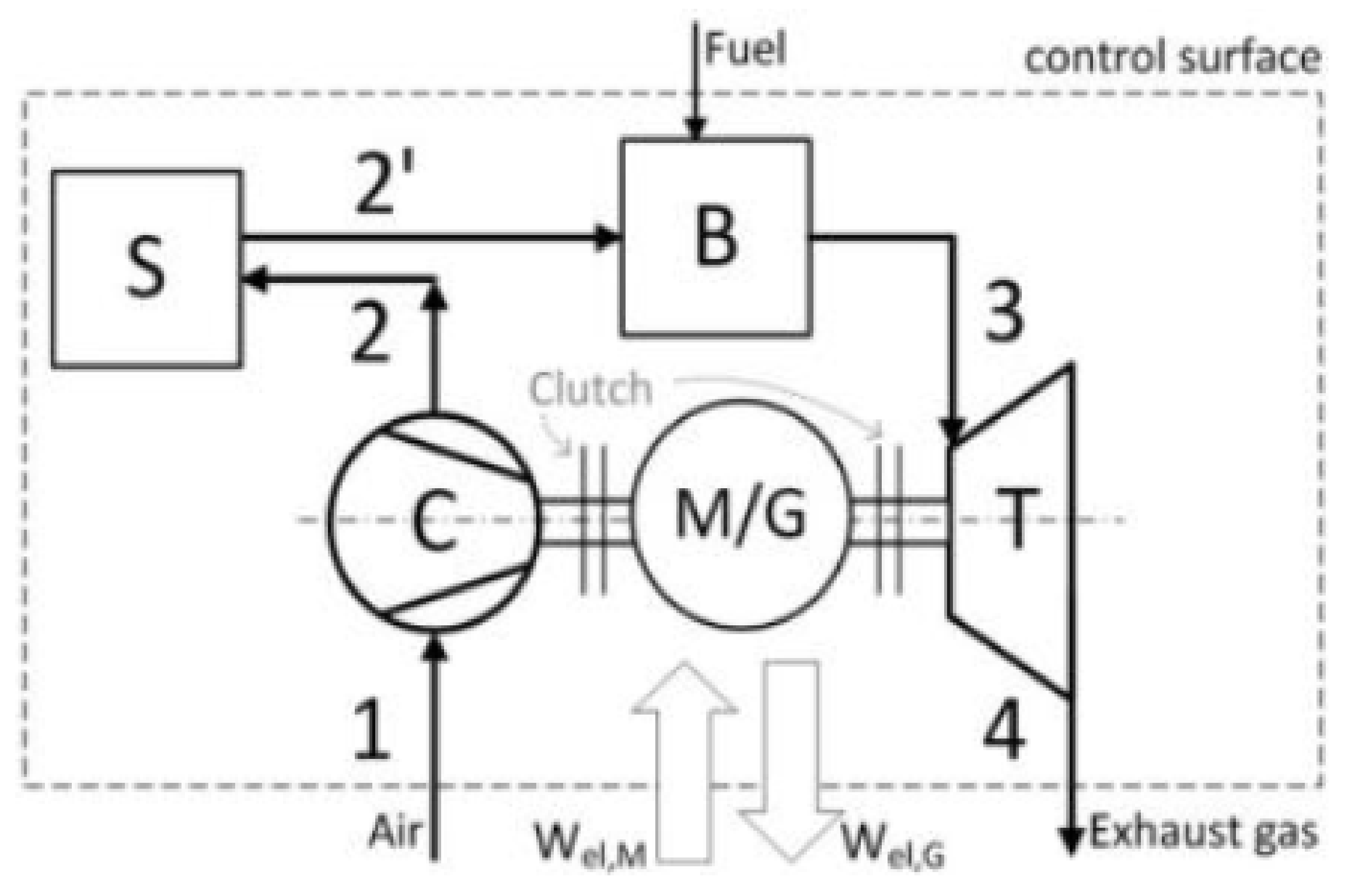
1.1. CAES Plant in Huntorf
1.2. Research Review
2. Materials and Method
2.1. Input Data
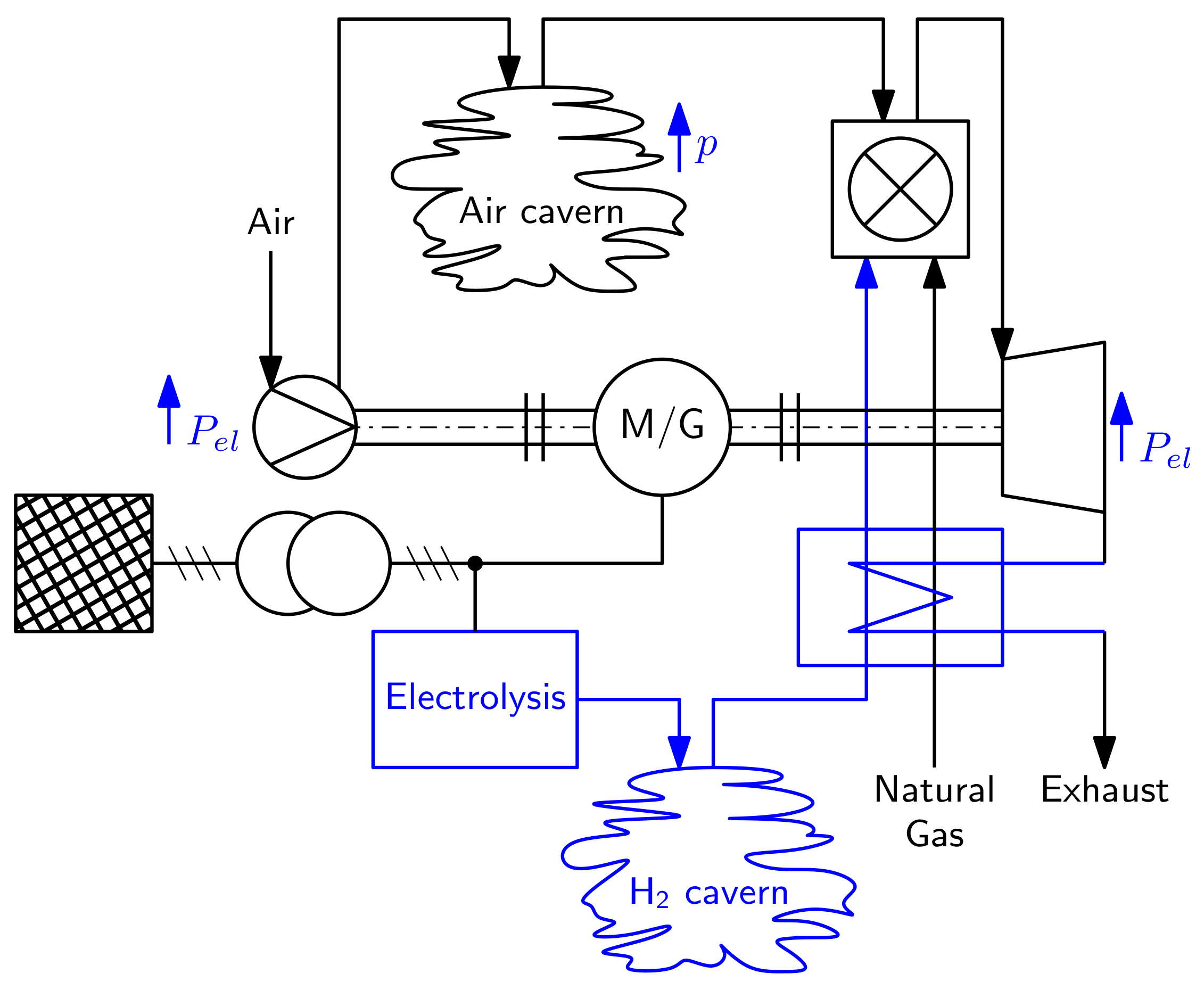
2.2. Plant Model
2.2.1. Constraints
2.2.2. Objective Function
3. Results
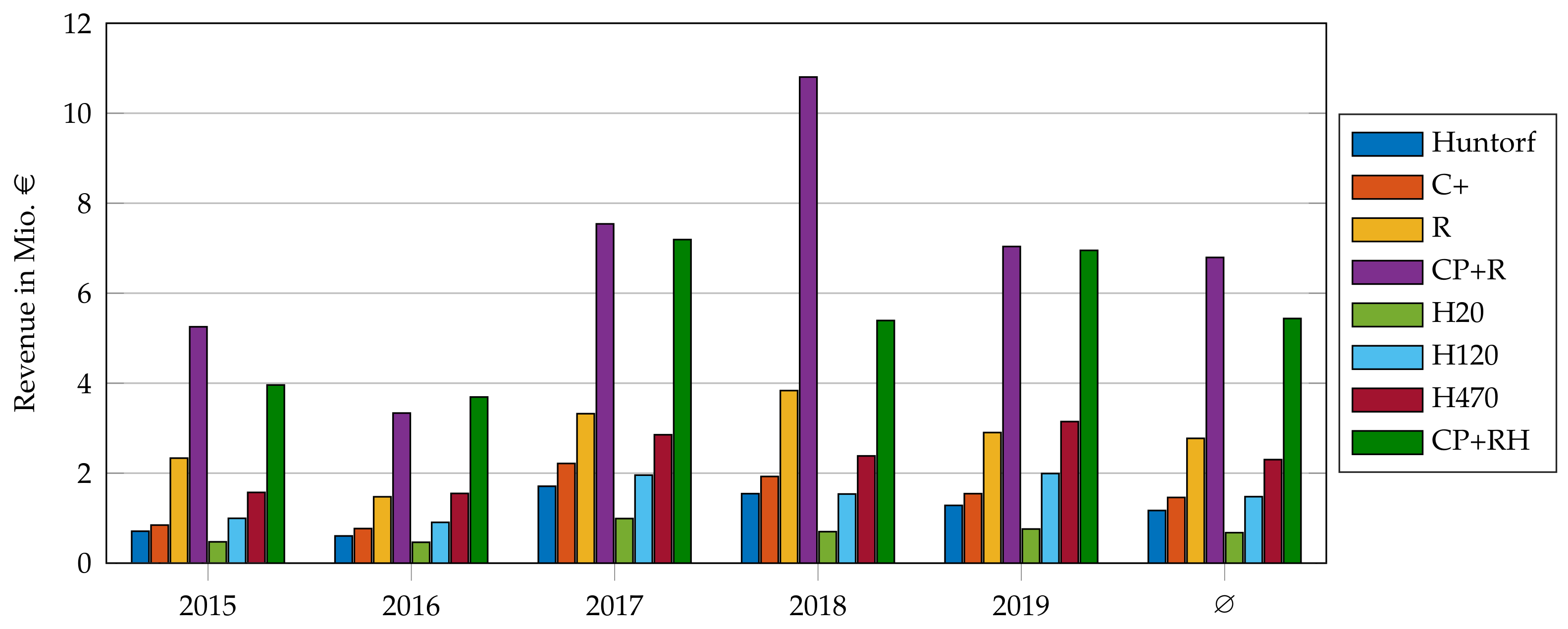
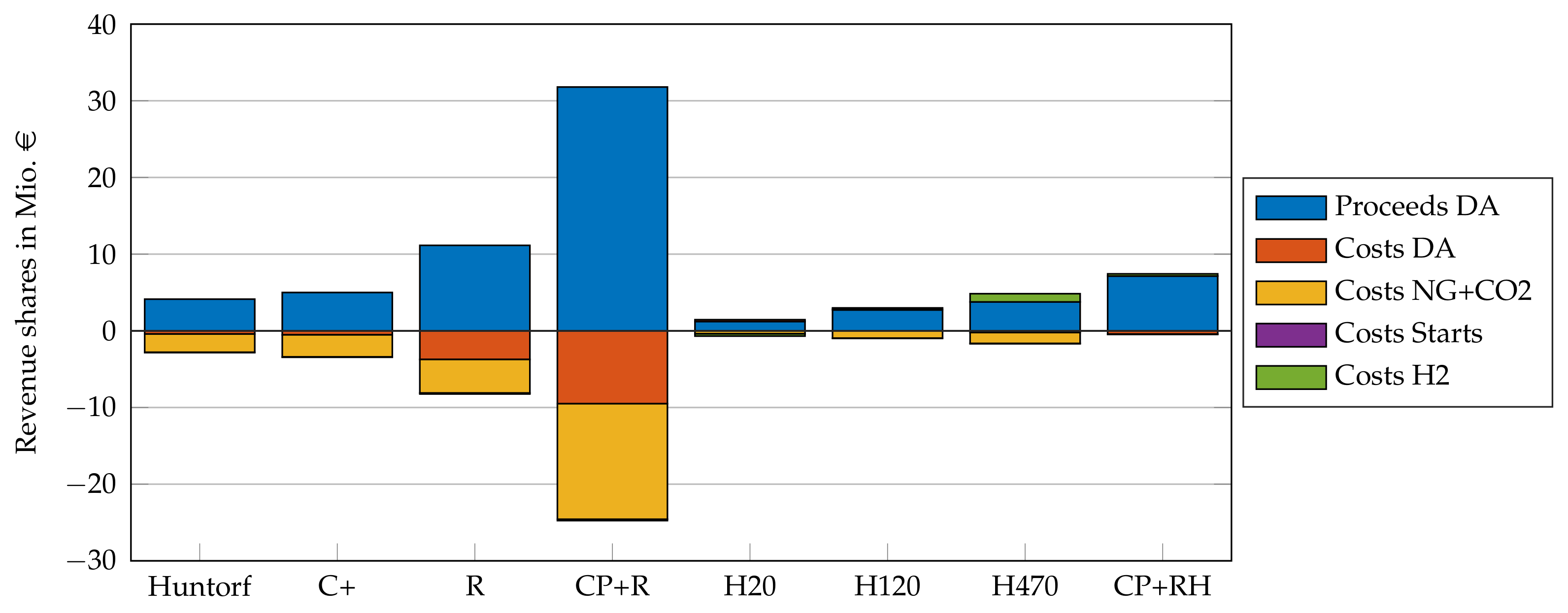
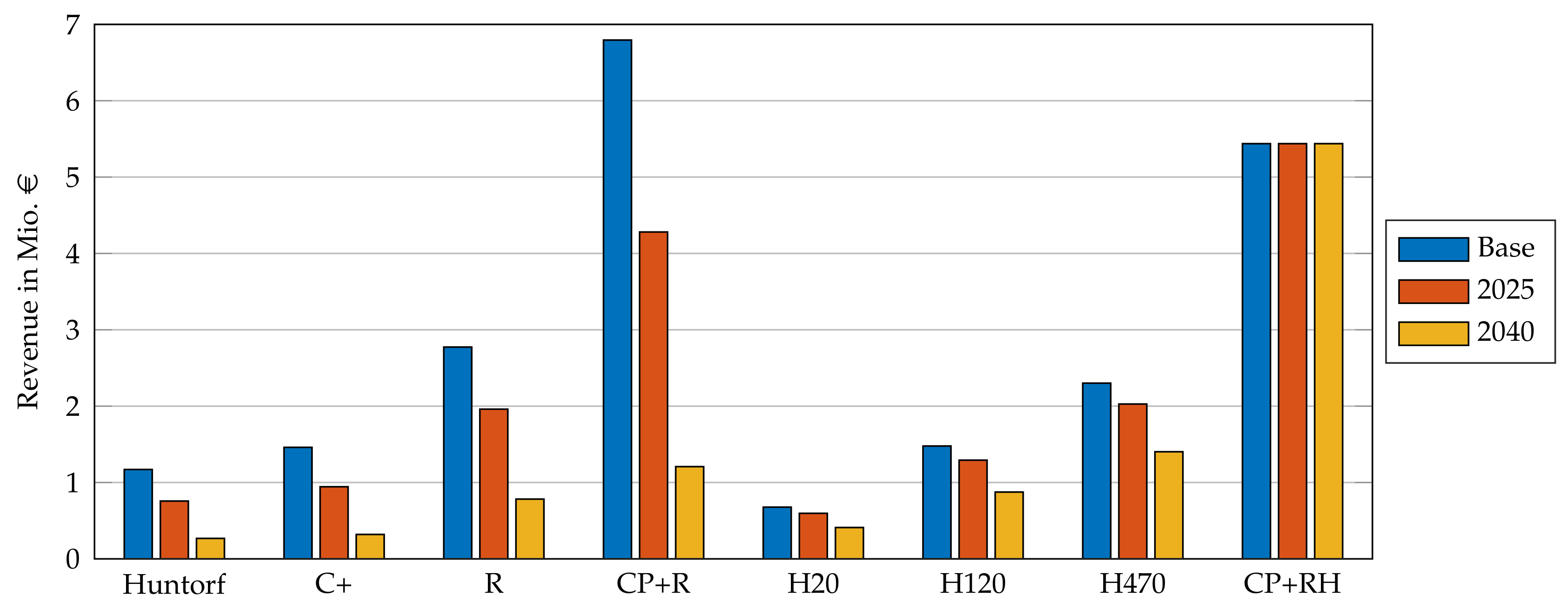
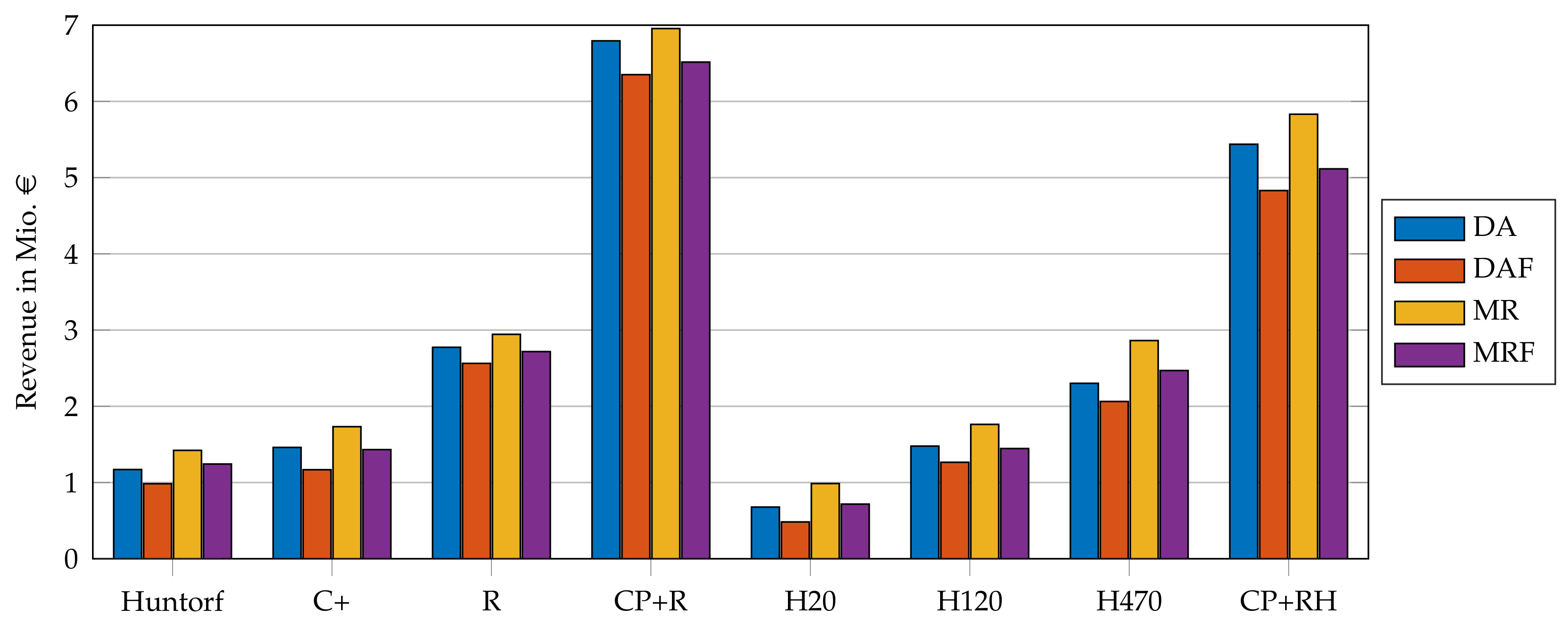
3.1. Revenue
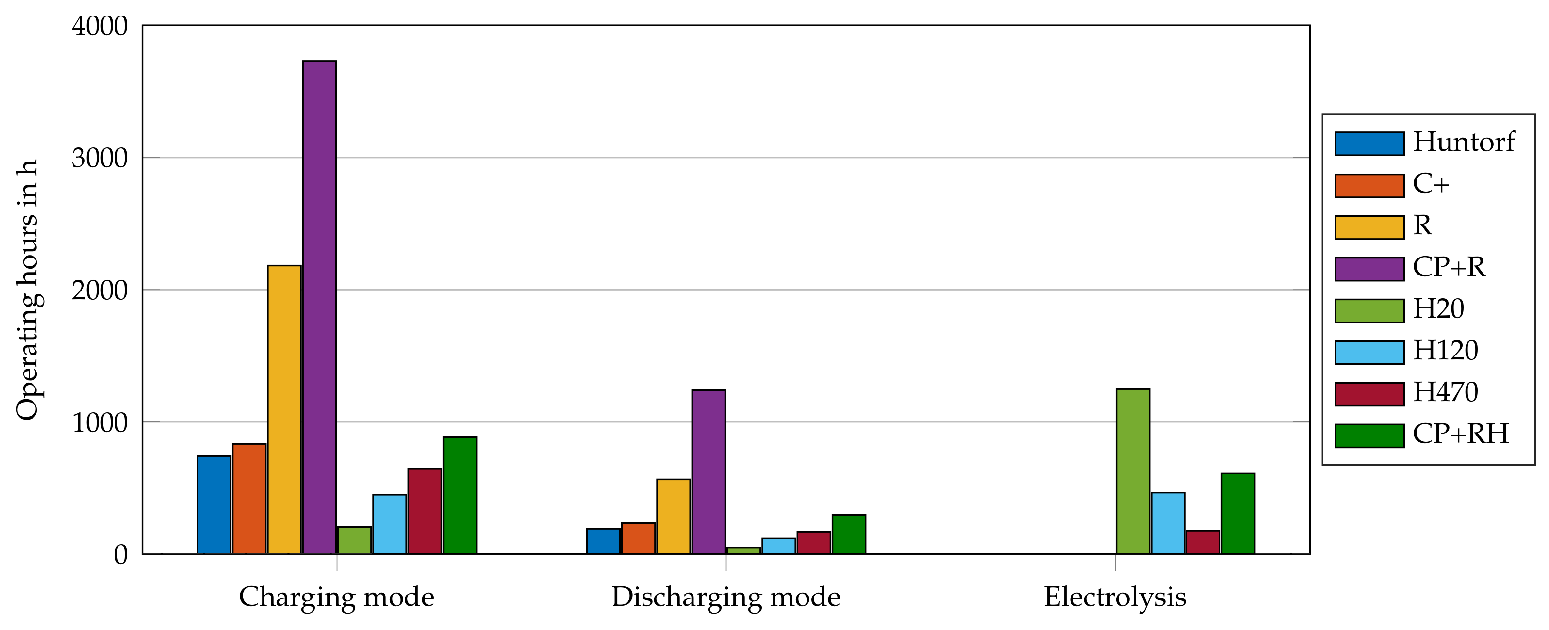
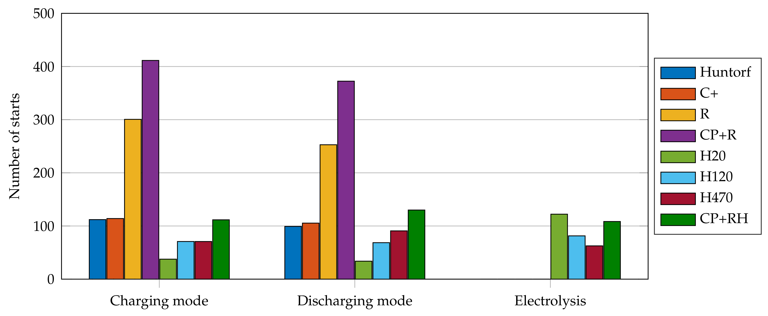
3.2. Operation Parameters
3.3. Summary
4. Conclusions
Author Contributions
Funding
Institutional Review Board Statement
Informed Consent Statement
Data Availability Statement
Acknowledgments
Conflicts of Interest
Appendix A

| Index | Description |
|---|---|
| t | time-dependent variable |
| r | rated |
| C | charging mode |
| D | discharging mode |
| A | compressed air |
| H | electrolysis/hydrogen |
| Symbol | Description |
|---|---|
| state of charge of the compressed air storage | |
| power in charging mode | |
| power in discharging mode | |
| binary variable: charging mode | |
| binary variable: discharging mode | |
| binary variable: startup charging mode | |
| binary variable: startup discharging mode | |
| State of charge of the hydrogen storage | |
| power of electrolysis | |
| binary variable: electrolysis | |
| binary variable: startup electrolysis | |
| reserved power for negative minute reserve | |
| reserved power for positive minute reserve | |
| called energy for negative minute reserve | |
| called energy for positive minute reserve | |
| binary variable: power reserved for negative minute reserve | |
| binary variable: power reserved for positive minute reserve |
| Symbol | Description |
|---|---|
| day-ahead market prices [25] | |
| fuel price (natural gas and carbon dioxide emissions) 1 | |
| startup costs: charging 1 | |
| startup costs: discharging 1 | |
| startup costs: electrolysis 1 | |
| tendered capacity price 4 () | |
| tendered energy price 4 () | |
| rated storage capacity of compressed air storage 1 | |
| rated power in charging mode 1 | |
| minimal power in discharging mode 1 | |
| rated power in discharging mode 1 | |
| efficiency in discharging mode 4 | |
| minimal power in discharging mode (partial load) 2 | |
| rated power in discharging mode (partial load) 2 | |
| fuel consumption at minimal discharging power 2 () | |
| fuel consumption constant 2 () | |
| rated storage capacity of H2 storage 4 | |
| minimal power of electrolyzer 3 | |
| rated power of electrolyzer 3 | |
| efficiency of electrolyzer 3 | |
| time step 3 |
References
- Prognos; Öko-Institut; Wuppertal-Institut. Towards a Climate-Neutral Germany by 2045. How Germany Can Reach Its Climate Targets before 2050. 2021. Executive Summary conducted for Stiftung Klimaneutralität, Agora Energiewende and Agora Verkehrswende. Available online: https://www.agora-energiewende.de/en/publications/towards-a-climate-neutral-germany-executive-summary/ (accessed on 10 September 2021).
- Fürstenwerth, D.; Waldmann, L. Electricity Storage in the German Energy Transition. 2014. Study by Agora Energywende. Available online: https://www.agora-energiewende.de/en/publications/electricity-storage-in-the-german-energy-transition/ (accessed on 10 September 2021).
- Succar, S.; Williams, R. Compressed Air Energy Storage: Theory, Resources, and Applications for Wind Power; Princeton Environmental Institute, Energy Systems Analysis Group: Princeton, NJ, USA, 2008. [Google Scholar]
- Eckroad, S.; Gyuk, I.; Mears, L.; Gotschall, H.; Kamath, H. EPRI-DOE Handbook of Energy Storage for Transmission and Distribution Applications. 2003. Available online: https://www.epri.com/research/products/1001834 (accessed on 10 September 2021).
- Moreno, R.; Moreira, R.; Strbac, G. A MILP model for optimising multi-service portfolios of distributed energy storage. Appl. Energy 2015, 137, 554–566. [Google Scholar] [CrossRef] [Green Version]
- Gu, Y.; Mccalley, J.; Ni, M.; Bo, R. Economic Modeling of Compressed Air Energy Storage. Energies 2013, 6, 2221–2241. [Google Scholar] [CrossRef]
- Nikolakakis, T.; Fthenakis, V. CAES models for energy arbitrage and ancillary services: Comparison using mixed-integer programming optimization with market data from the Irish power grid. Energy Technol. 2017, 6, 1290–1301. [Google Scholar] [CrossRef]
- Wolf, D.; Kanngießer, A.; Budt, M.; Doetsch, C. Adiabatic Compressed Air Energy Storage co-located with wind energy—multifunctional storage commitment optimization for the German market using GOMES. Energy Syst. 2012, 3, 181–208. [Google Scholar] [CrossRef]
- Nikolakakis, T.; Fthenakis, V. The Value of Compressed-Air Energy Storage for Enhancing Variable-Renewable-Energy Integration: The Case of Ireland. Energy Technol. 2017, 5, 2026–2038. [Google Scholar] [CrossRef]
- Ghalelou, A.N.; Fakhri, A.P.; Nojavan, S.; Majidi, M.; Hatami, H. A stochastic self-scheduling program for compressed air energy storage (CAES) of renewable energy sources (RESs) based on a demand response mechanism. Energy Convers. Manag. 2016, 120, 388–396. [Google Scholar] [CrossRef]
- Kaiser, F.; Weber, R.; Krueger, U. Thermodynamic Steady-State Analysis and Comparison of Compressed Air Energy Storage (CAES) Concepts. Int. J. Thermodyn. 2018, 21, 144–156. [Google Scholar] [CrossRef]
- Budt, M.; Wolf, D.; Span, R.; Yan, J. A review on compressed air energy storage: Basic principles, past milestones and recent developments. Appl. Energy 2016, 170, 250–268. [Google Scholar] [CrossRef]
- Kaiser, F.; Krueger, U. Exergy analysis and assessment of performance criteria for compressed air energy storage concepts. Int. J. Exergy 2019, 28, 274–291. [Google Scholar] [CrossRef]
- Crotogino, F.; Mohmeyer, K.U.; Scharf, R. Huntorf CAES: More than 20 Years of Successful Operation: Report Spring 2001 Meeting, Orlando. In Proceedings of the Spring 2001 Meeting, Orlando, FL, USA, 15–18 April 2001. [Google Scholar]
- Lund, H.; Salgi, G.; Elmegaard, B.; Andersen, A.N. Optimal operation strategies of compressed air energy storage (CAES) on electricity spot markets with fluctuating prices. Appl. Therm. Eng. 2009, 29, 799–806. [Google Scholar] [CrossRef] [Green Version]
- Bullough, C.; Gatzen, C.; Jakiel, C.; Koller, M.; Nowi, A.; Zunft, S. Advanced adiabatic compressed air energy storage for the Integration of wind energy. In Proceedings of the European Wind Energy Conference, EWEC 2004, London, UK, 22–25 November 2004. [Google Scholar]
- Denholm, P.; Sioshansi, R. The value of compressed air energy storage with wind in transmission-constrained electric power systems. Energy Policy 2009, 37, 3149–3158. [Google Scholar] [CrossRef]
- Nabil, I.; Khairat Dawood, M.M.; Nabil, T. Review of Energy Storage Technologies for Compressed-Air Energy Storage. Am. J. Mod. Energy 2021, 4, 51–60. [Google Scholar] [CrossRef]
- Drury, E.; Denholm, P.; Sioshansi, R. The value of compressed air energy storage in energy and reserve markets. Fuel Energy Abstr. 2011, 36, 4959–4973. [Google Scholar] [CrossRef]
- Nasouri Gilvaei, M.; Hosseini Imani, M.; Jabbari Ghadi, M.; Li, L.; Golrang, A. Profit-Based Unit Commitment for a GENCO Equipped with Compressed Air Energy Storage and Concentrating Solar Power Units. Energies 2021, 14, 576. [Google Scholar] [CrossRef]
- Jakiel, C.; Zunft, S.; Nowi, A. Adiabatic compressed air energy storage plants for efficient peak load power supply from wind energy: The European project AA-CAES. Int. J. Energy Technol. Policy 2007, 5, 296–306. [Google Scholar] [CrossRef]
- Zunft, S.; Dreißigacker, V.; Bieber, M.; Banach, A.; Klabunde, C.; Warweg, O. Electricity storage with adiabatic compressed air energy storage: Results of the BMWi-project ADELE-ING. In Proceedings of the International ETG Congress 2017, Bonn, Germany, 28–29 November 2017. [Google Scholar]
- Barbour, E.R.; Pottie, D.L.; Eames, P. Why is adiabatic compressed air energy storage yet to become a viable energy storage option? iScience 2021, 24, 102440. [Google Scholar] [CrossRef]
- Hamedi, K.; Sadeghi, S.; Esfandi, S.; Azimian, M.; Golmohamadi, H. Eco-Emission Analysis of Multi-Carrier Microgrid Integrated with Compressed Air and Power-to-Gas Energy Storage Technologies. Sustainability 2021, 13, 4681. [Google Scholar] [CrossRef]
- Bundesnetzagentur. Electricity Market Data. 2020. Available online: www.smard.de (accessed on 10 September 2021).
- 50Hertz Transmission GmbH; Amprion GmbH; TenneT TSO GmbH; TransnetBW GmbH. Regelleistung.net—Internet Platform for the Allocation of Control Power. 2020. Available online: https://www.regelleistung.net/ext/static/mrl (accessed on 10 September 2021).
- Quaschning, V. Specific Carbon Dioxide Emissions of Various Fuels. 2021. Available online: https://www.volker-quaschning.de/datserv/CO2-spez/index_e.php (accessed on 10 September 2021).
- International Energy Agency. World Energy Outlook 2017. 2017. Available online: https://www.iea.org/reports/world-energy-outlook-2017 (accessed on 10 September 2021).
- Hu, L.; Taylor, G.; Wan, H.B.; Irving, M. A Review of Short-Term Electricity Price Forecasting Techniques in Deregulated Electricity Markets. In Proceedings of the 2009 44th International Universities Power Engineering Conference (UPEC), Glasgow, UK, 1–4 September 2009; pp. 1–5. [Google Scholar]
- Aggarwal, S.; Saini, L.; Kumar, A. Electricity price forecasting in deregulated markets: A review and evaluation. Int. J. Electr. Power Energy Syst. 2009, 31, 13–22. [Google Scholar] [CrossRef]
- Ugurlu, U.; Tas, O.; Kaya, A.; Oksuz, I. The Financial Effect of the Electricity Price Forecasts’ Inaccuracy on a Hydro-Based Generation Company. Energies 2018, 11, 2093. [Google Scholar] [CrossRef] [Green Version]
- Delarue, E.; van den Bosch, P.; D’haeseleer, W. Effect of the accuracy of price forecasting on profit in a Price Based Unit Commitment. Electr. Power Syst. Res. 2010, 80, 1306–1313. [Google Scholar] [CrossRef]
- Lago, J.; de Ridder, F.; de Schutter, B. Forecasting spot electricity prices: Deep learning approaches and empirical comparison of traditional algorithms. Appl. Energy 2018, 221, 386–405. [Google Scholar] [CrossRef]
- Kopanos, G.M.; Pistikopoulos, E.N. Reactive Scheduling by a Multiparametric Programming Rolling Horizon Framework: A Case of a Network of Combined Heat and Power Units. Ind. Eng. Chem. Res. 2014, 53, 4366–4386. [Google Scholar] [CrossRef]
- Bischi, A.; Taccari, L.; Martelli, E.; Amaldi, E.; Manzolini, G.; Silva, P.; Campanari, S.; Macchi, E. A rolling-horizon optimization algorithm for the long term operational scheduling of cogeneration systems. Energy 2019, 184, 73–90. [Google Scholar] [CrossRef]
- Ashour Novirdoust, A.; Bicherl, M.; Bojung, C.; Buhl, H.U.; Fridgen, G.; Getschko, V.; Hanny, L.; Knörr, J.; Maldonado, F.; Neuhoff, K.; et al. Electricity Spot Market Design 2030–2050; Fraunhofer FIT: Sankt Augustin, Germany, 2020. [Google Scholar] [CrossRef]
- Fries, A.K.; Kaiser, F.; Beck, H.P.; Weber, R. Huntorf 2020—Improvement of Flexibility and Efficiency of a Compressed Air Energy Storage Plant based on Synthetic Hydrogen. In Proceedings of the NEIS 2018 Conference on Sustainable Energy Supply and Energy Storage Systems, Hamburg, Germany, 20–21 September 2018; pp. 1–5. [Google Scholar]
| Abbr. | Plant Variations |
|---|---|
| Huntorf | current state of the Huntorf CAES plant |
| C+ | increased storage capacity |
| R | recuperation |
| CP+R | increased storage capacity, rated charging and discharging power, and recuperation |
| H20 | hydrogen combustion (rated electrolysis power 20 MW) |
| H120 | hydrogen combustion (rated electrolysis power 120 MW) |
| H470 | hydrogen combustion (rated electrolysis power 470 MW) |
| CP+RH | combination of CP+R with hydrogen combustion (rated electrolysis power 500 MW) |
| Abb. | Use Cases |
|---|---|
| DA | revenue maximization in day-ahead market |
| DAF | revenue maximization in day-ahead market with forecast uncertainty |
| MR | revenue maximization in minute-operating-reserve market |
| MRF | revenue maximization in minute-operating-reserve market with forecast uncertainty |
| Scenario | Natural Gas Price | Carbon Emission Price | Resulting Fuel Price |
|---|---|---|---|
| base | EUR 20/ | EUR 25/t | EUR 25/ |
| 2025 | EUR 20/ | EUR 55/t | EUR 31/ |
| 2040 | EUR 30/ | EUR 100/t | EUR 50/ |
Publisher’s Note: MDPI stays neutral with regard to jurisdictional claims in published maps and institutional affiliations. |
© 2021 by the authors. Licensee MDPI, Basel, Switzerland. This article is an open access article distributed under the terms and conditions of the Creative Commons Attribution (CC BY) license (https://creativecommons.org/licenses/by/4.0/).
Share and Cite
Klaas, A.-K.; Beck, H.-P. A MILP Model for Revenue Optimization of a Compressed Air Energy Storage Plant with Electrolysis. Energies 2021, 14, 6803. https://doi.org/10.3390/en14206803
Klaas A-K, Beck H-P. A MILP Model for Revenue Optimization of a Compressed Air Energy Storage Plant with Electrolysis. Energies. 2021; 14(20):6803. https://doi.org/10.3390/en14206803
Chicago/Turabian StyleKlaas, Ann-Kathrin, and Hans-Peter Beck. 2021. "A MILP Model for Revenue Optimization of a Compressed Air Energy Storage Plant with Electrolysis" Energies 14, no. 20: 6803. https://doi.org/10.3390/en14206803
APA StyleKlaas, A.-K., & Beck, H.-P. (2021). A MILP Model for Revenue Optimization of a Compressed Air Energy Storage Plant with Electrolysis. Energies, 14(20), 6803. https://doi.org/10.3390/en14206803