Identification of the Technical Condition of Induction Motor Groups by the Total Energy Flow


Abstract
:1. Introduction
2. Materials and Methods
3. Experiments
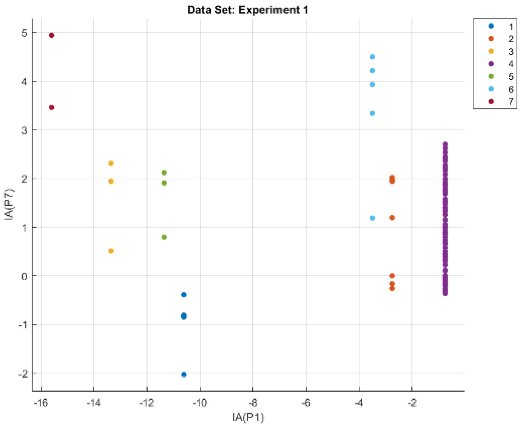
3.1. Experiment 1
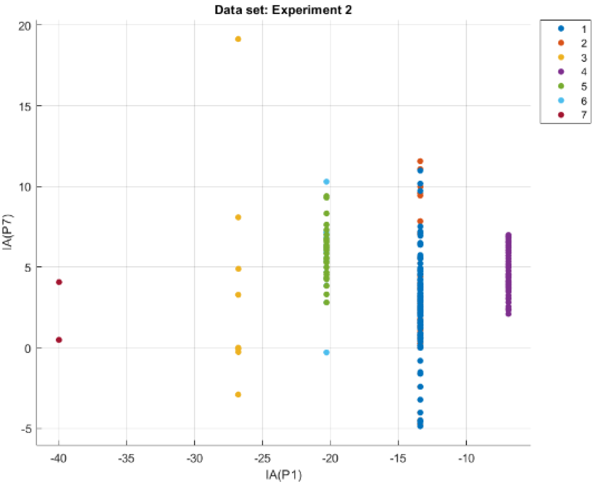
3.2. Experiment 2
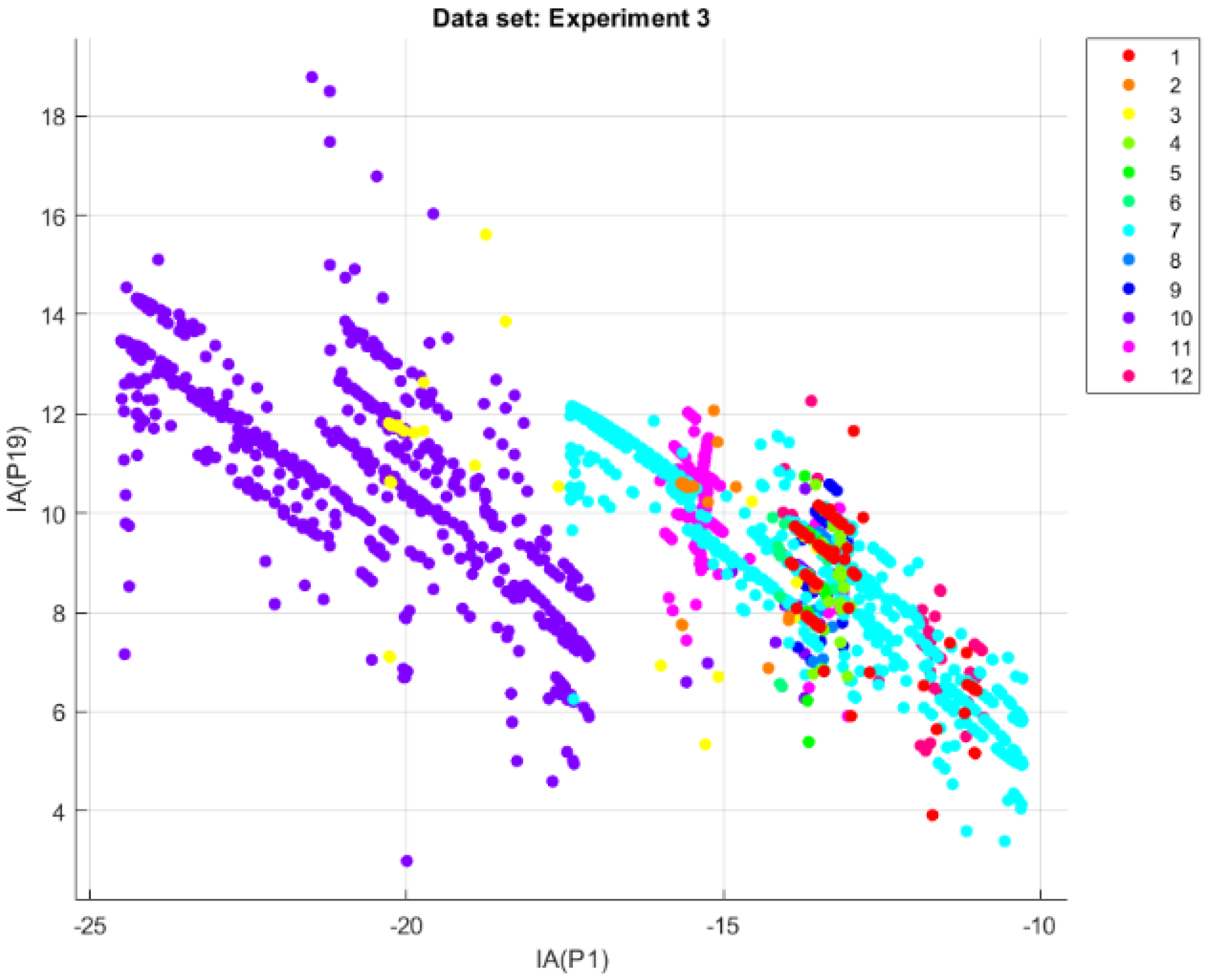
3.3. Experiment 3
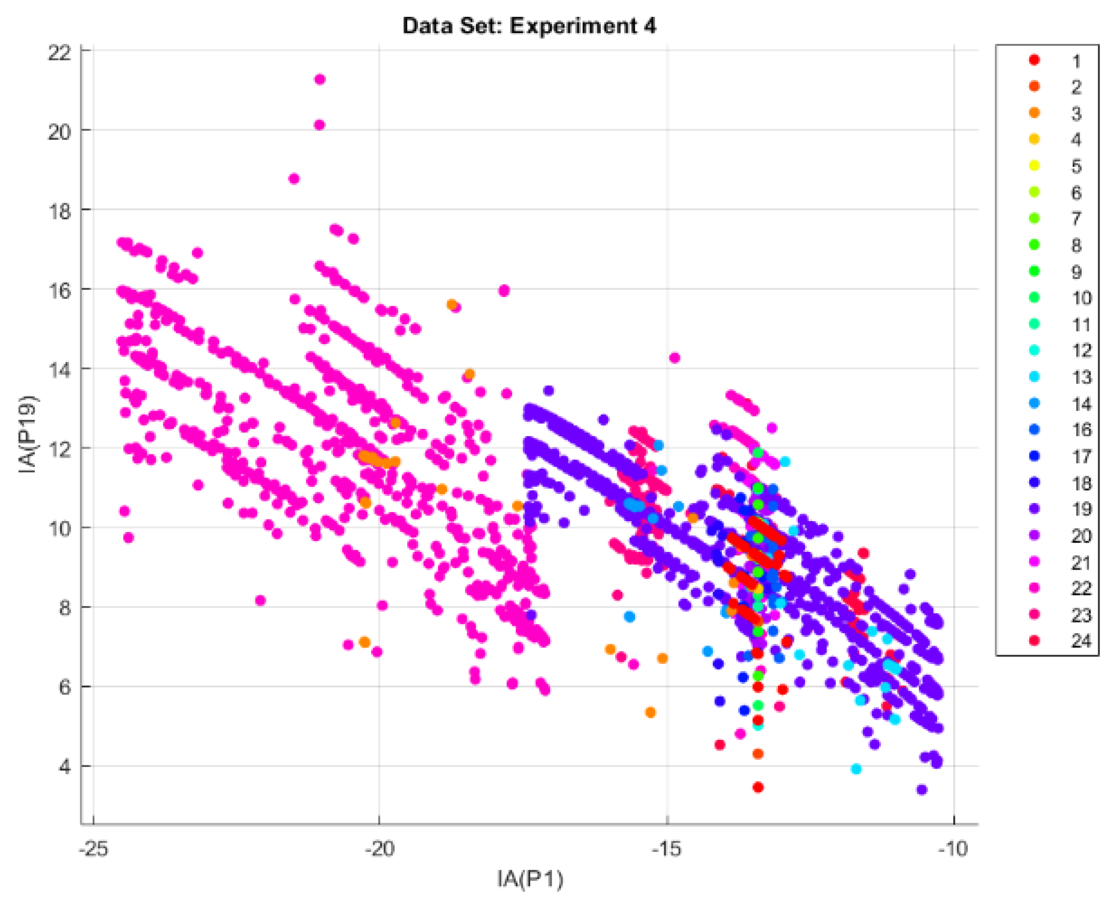
3.4. Experiment 4
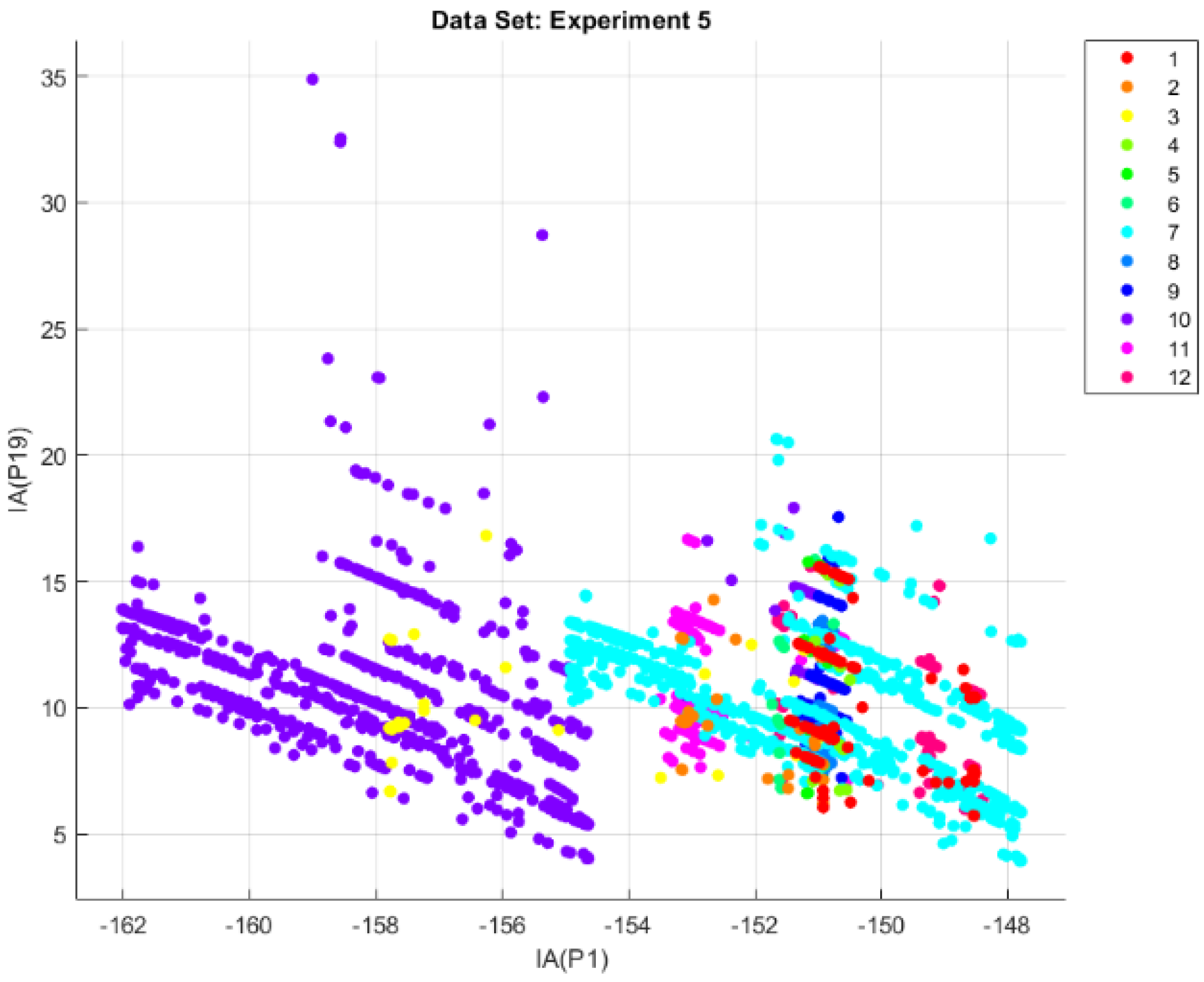
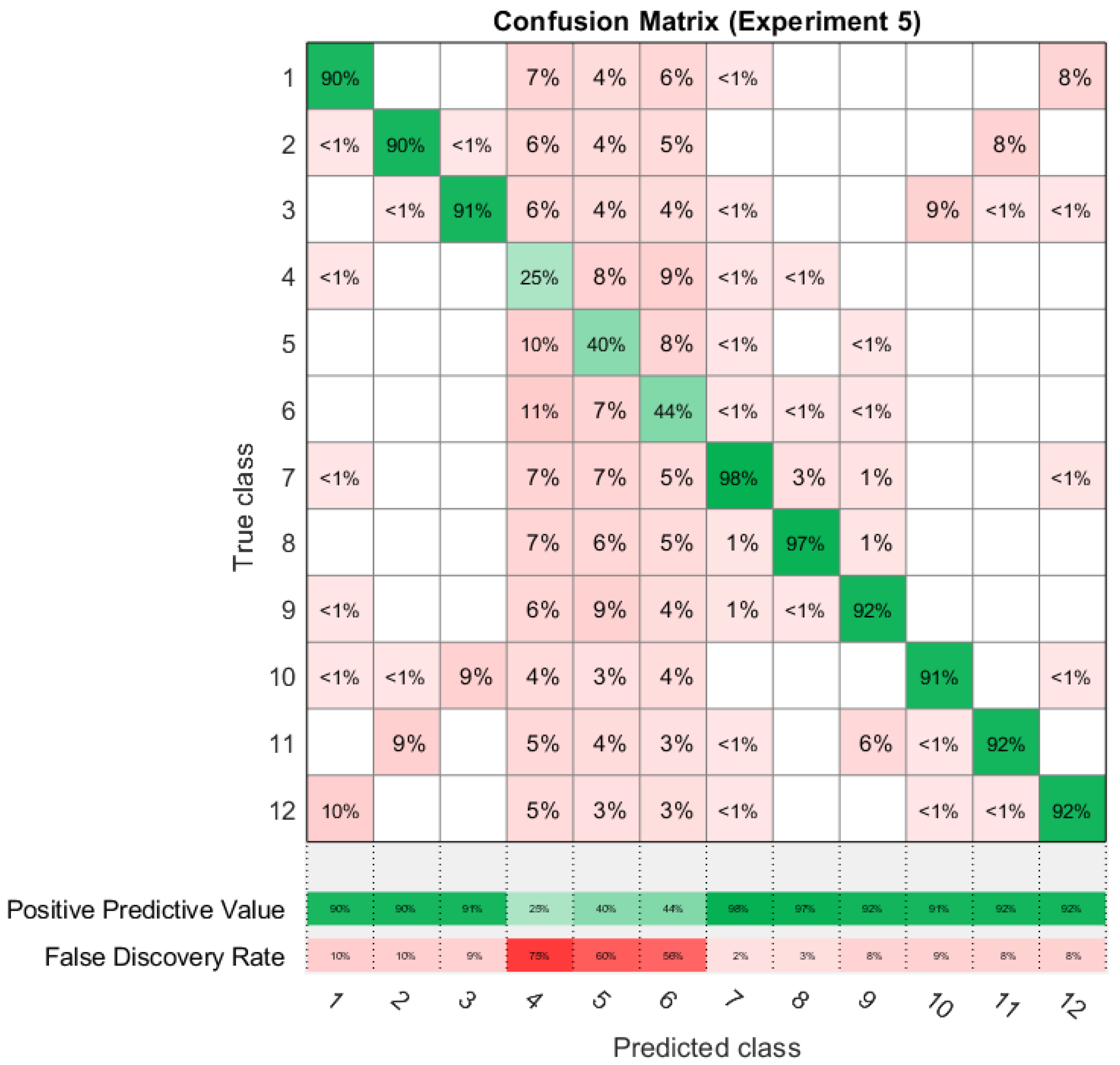
3.5. Experiment 5
4. Results and Discussion
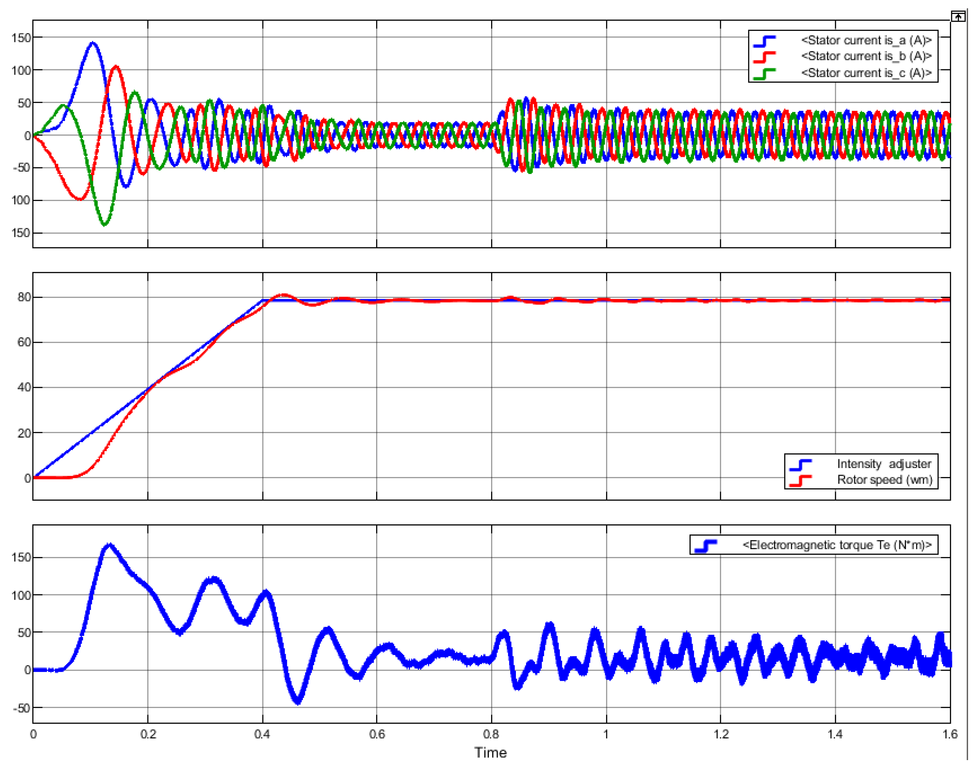
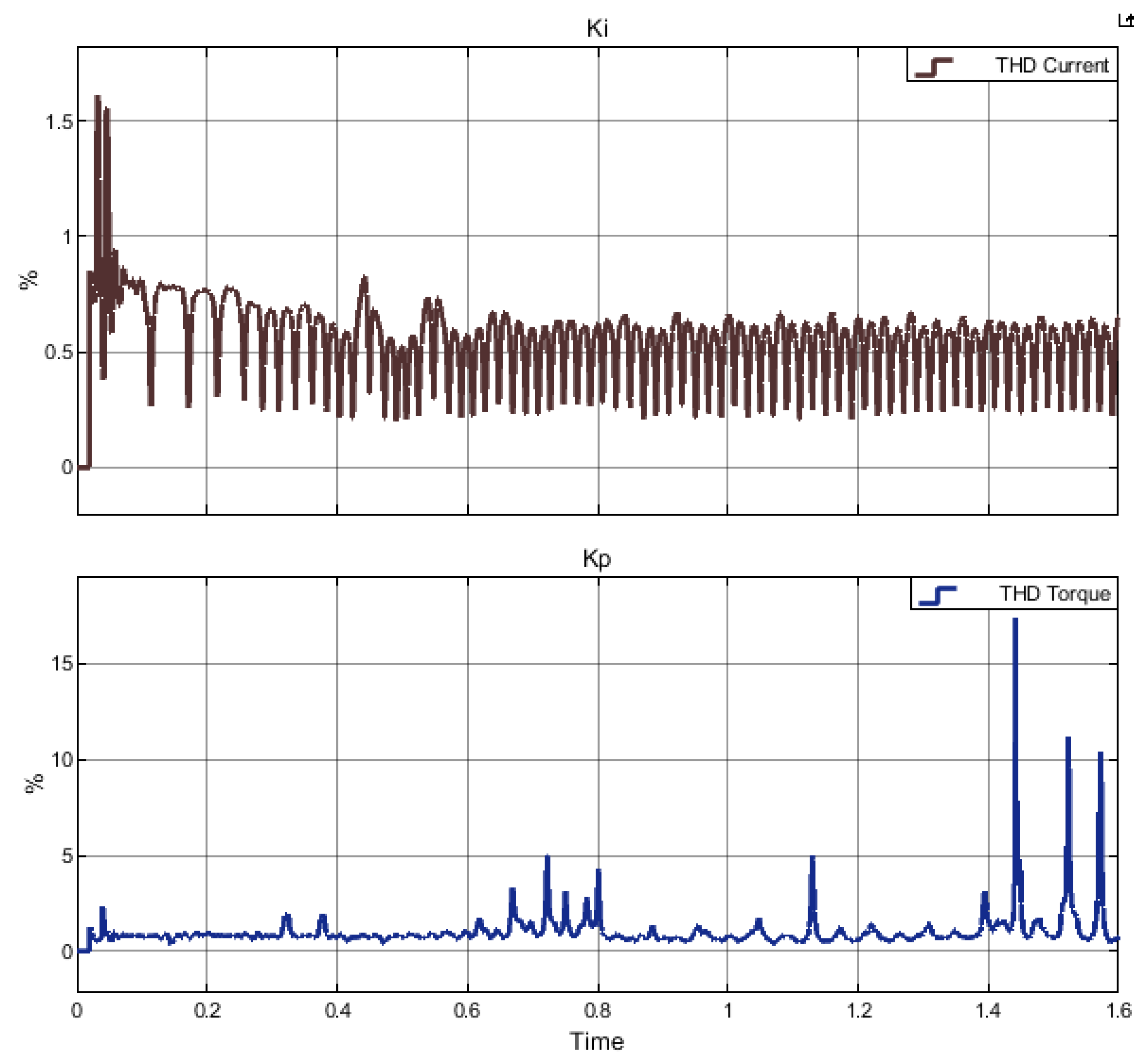
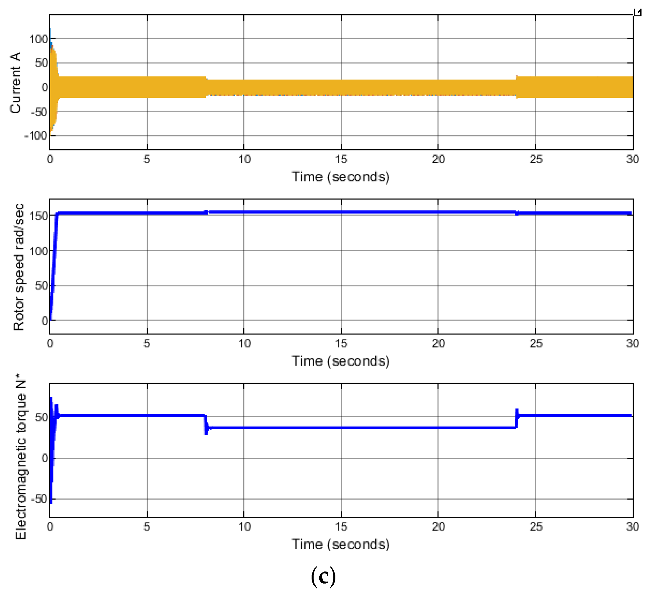
4.1. Research of Changes in the Energy (Current) Characteristics of an Induction Electric Motor When Defects Occur
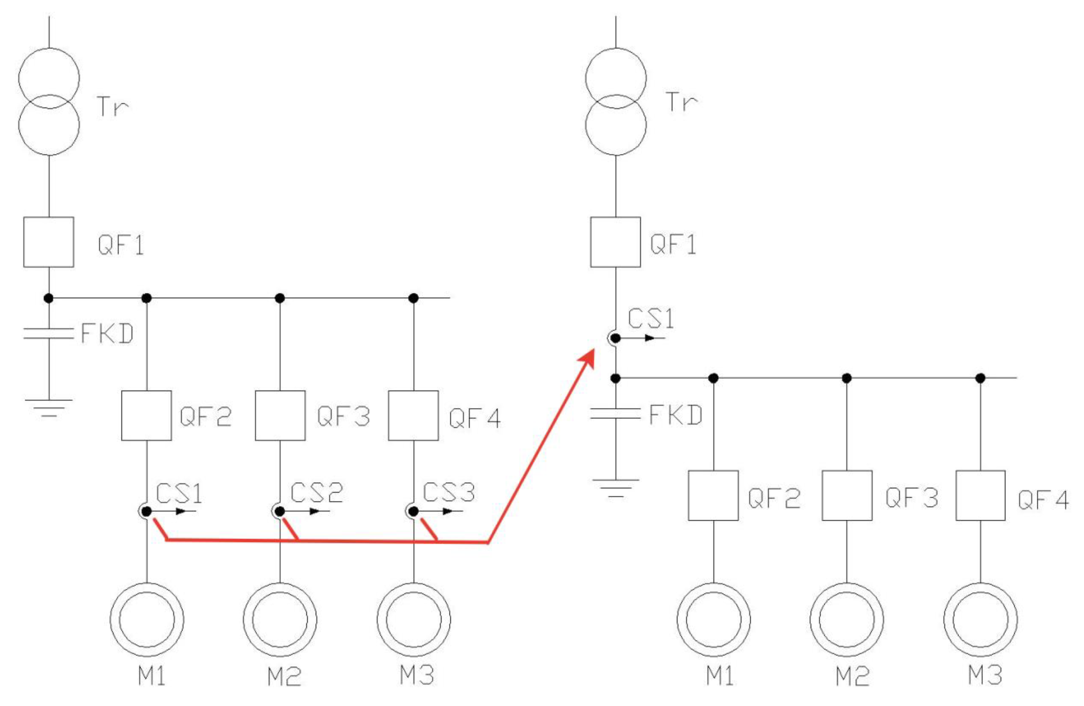
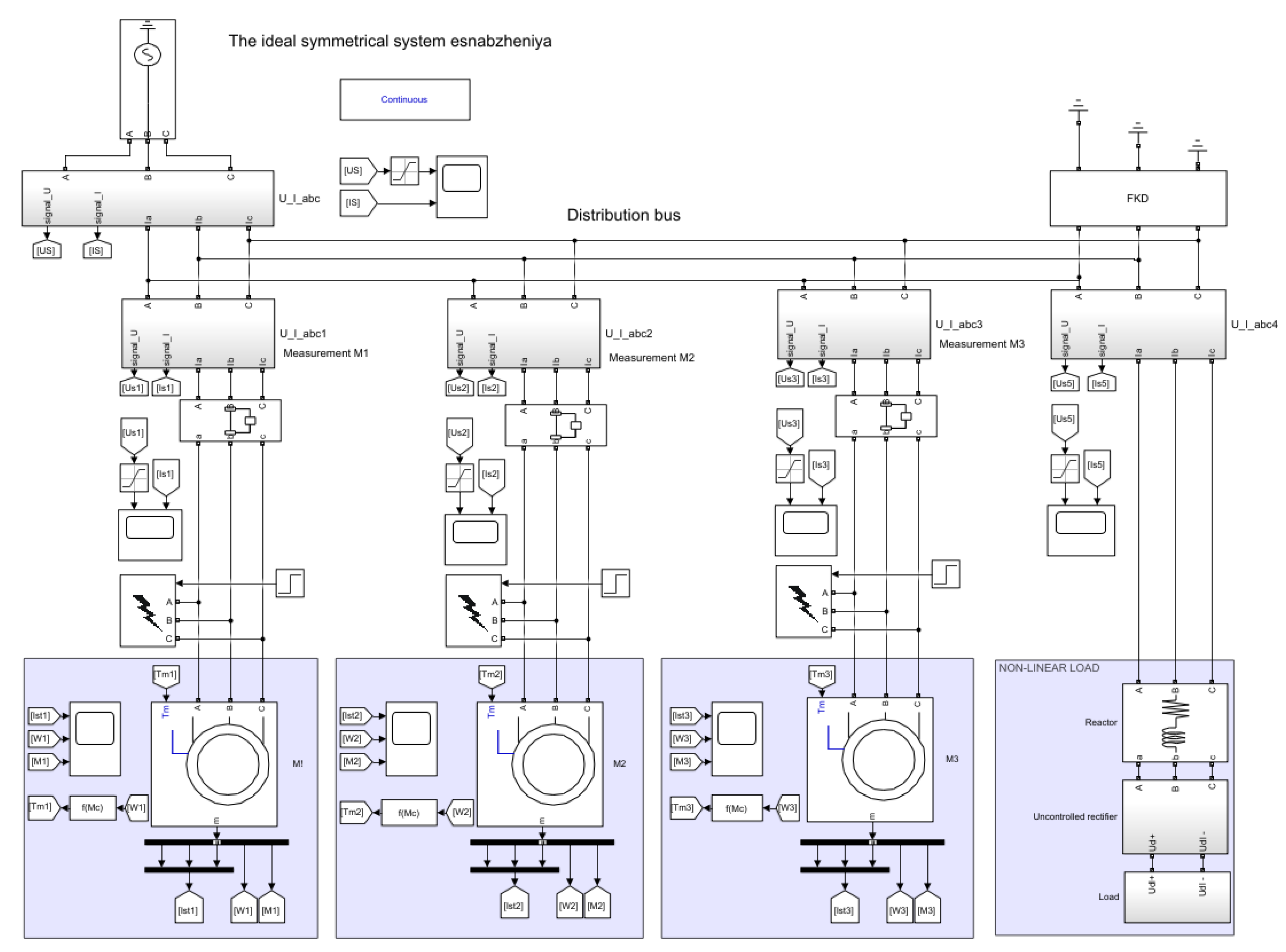
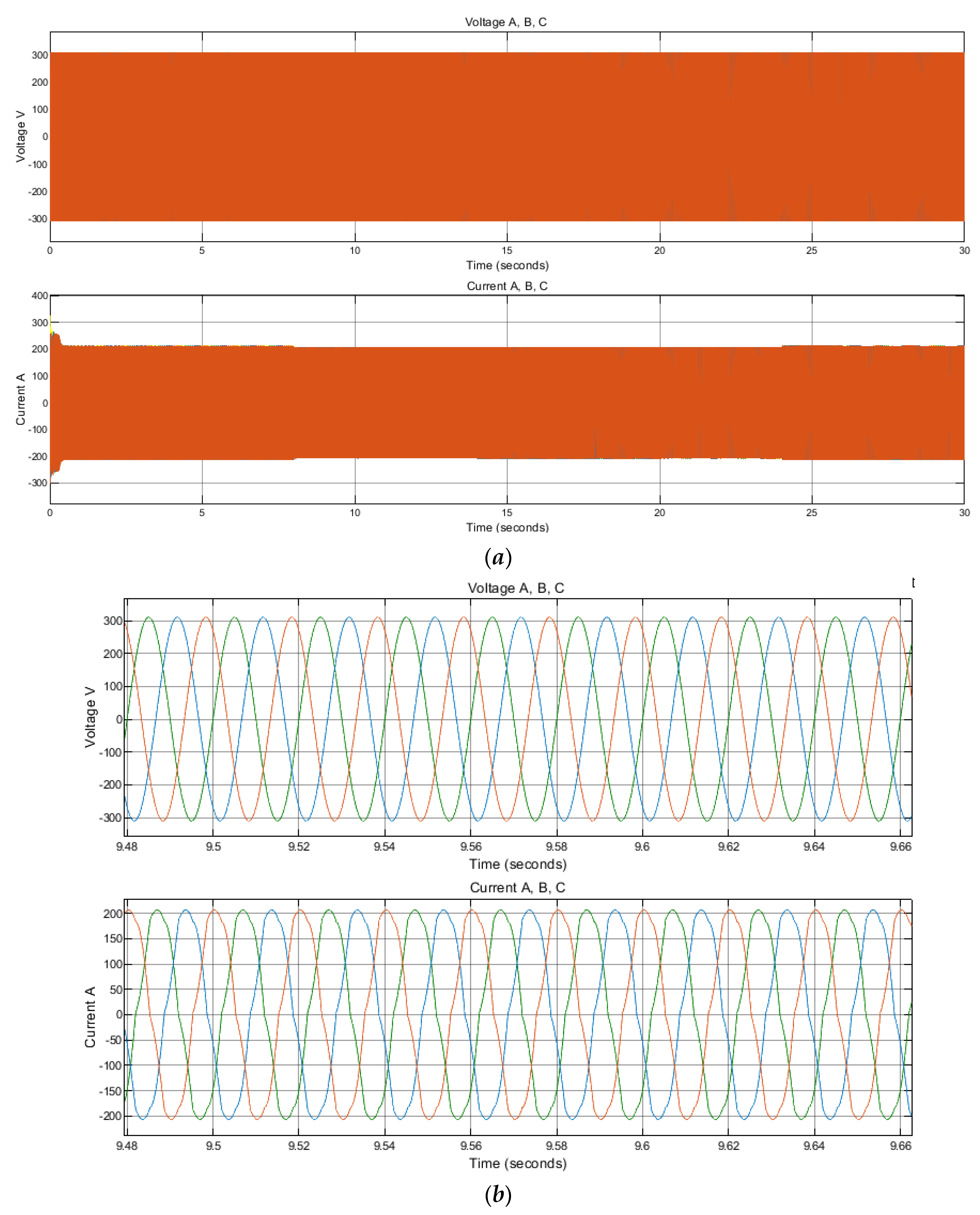
4.2. Simulation of a Simplified Power Supply System with Individual Motor Control and Total Energy Flow Control
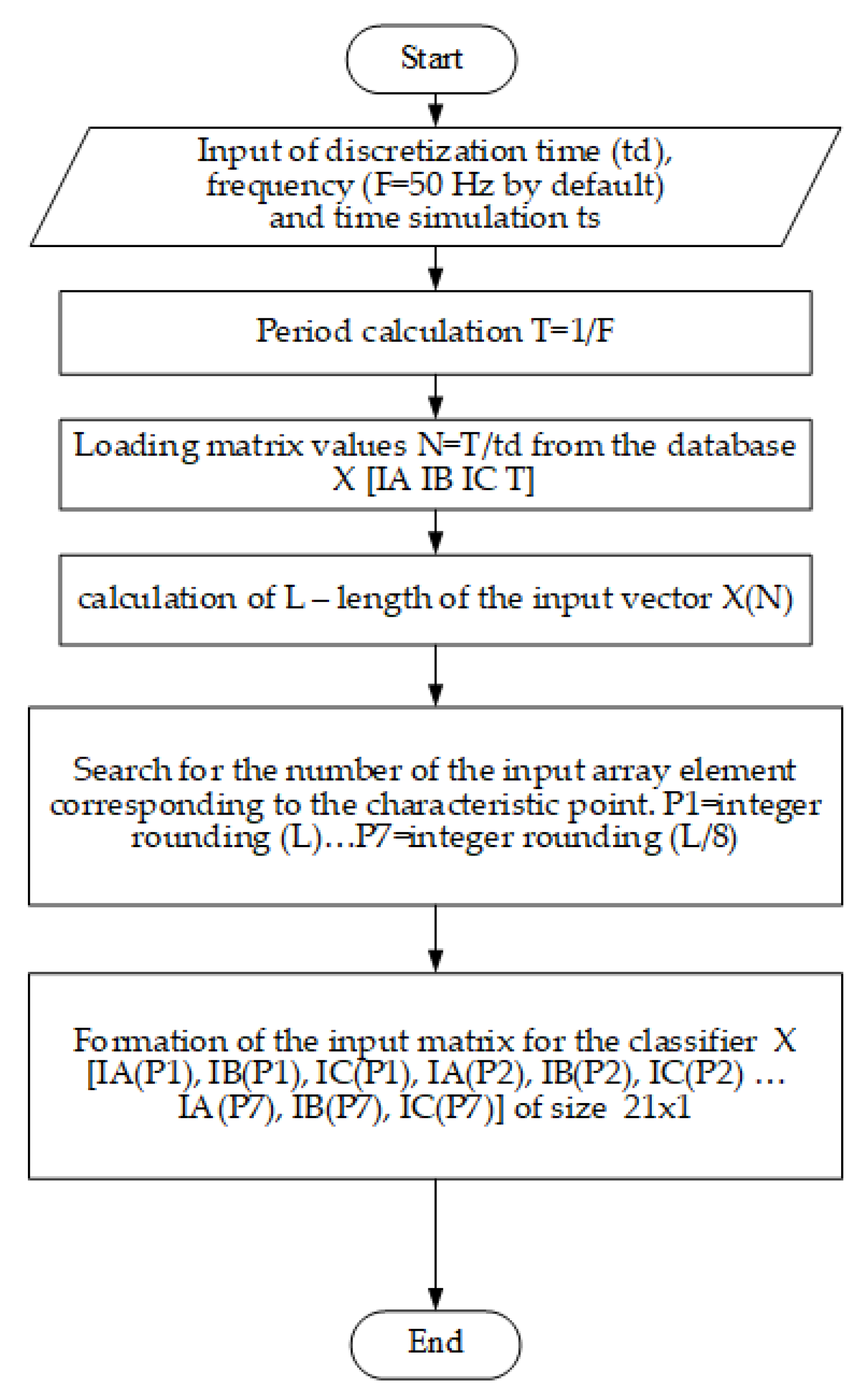
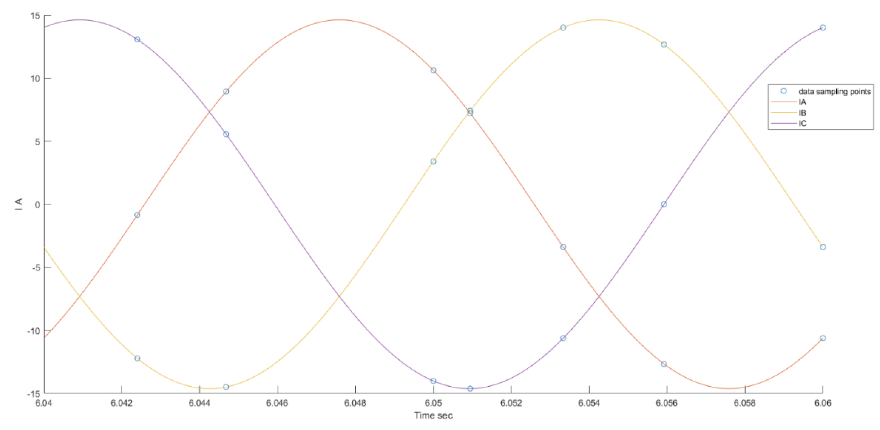
4.3. Preparing Data for Classification
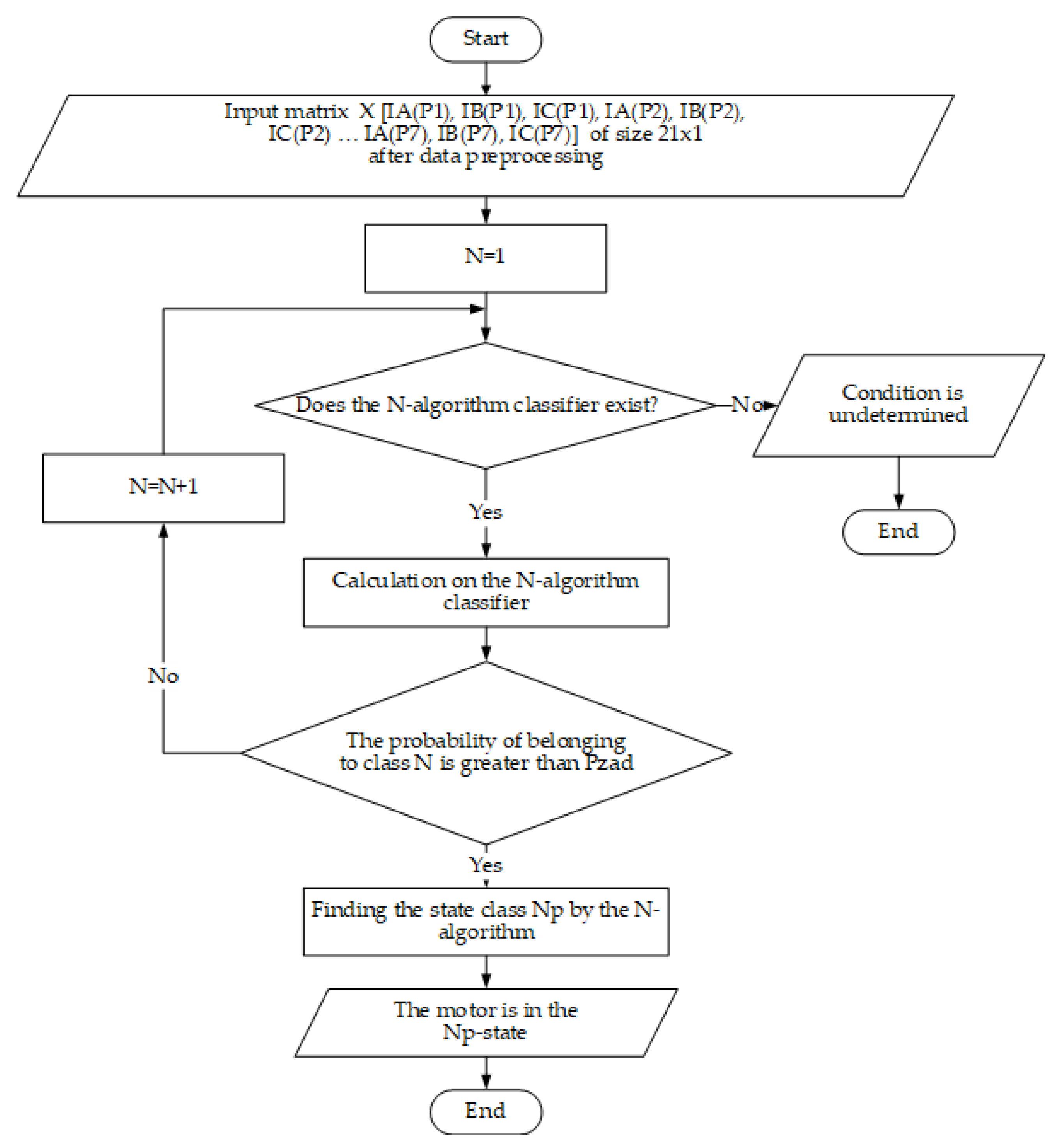
4.4. Data Classification
5. Conclusions
Author Contributions
Funding
Institutional Review Board Statement
Informed Consent Statement
Conflicts of Interest
References
- Malov, D.; Edemskii, A.; Saveliev, A. Architecture of proactive localization service for cyber-physical system’s users. In International Conference on Interactive Collaborative Robotics; Springer: Cham, Switzerland, 2019; Volume 11659, pp. 10–18. [Google Scholar] [CrossRef]
- O’Leary, P.; Harker, M.; Ritt, R.; Habacher, M.; Landl, K.; Brandner, M. Mining sensor data in larger physical systems. IFAC-Pap. 2016, 49, 37–42. [Google Scholar] [CrossRef]
- Klyuev, R.; Fomenko, O.; Gavrina, O.; Turluev, R.; Marzoev, S. Energy indicators of drilling machines and excavators in mountain territories. In Energy Management of Municipal Transportation Facilities and Transport; Springer: Cham, Switzerland, 2019; Volume 1258, pp. 272–281. [Google Scholar] [CrossRef]
- Safina, E.; Khokhlov, S. Paradox of alternative energy consumption: Lean or profligacy? Int. J. Qual. Res. 2017, 11, 903–916. [Google Scholar] [CrossRef]
- Dobush, V.S.; Belsky, A.A.; Skamyin, A.N. Electrical Complex for Autonomous Power Supply of Oil Leakage Detection Systems in Pipelines. J. Phys. Conf. Ser. 2020, 1441, 157105. [Google Scholar] [CrossRef]
- Ivkina, O.P.; Ziyakaev, G.R.; Pashkov, E.N. Mathematic study of the rotor motion with a pendulum selfbalancing device. J. Phys. Conf. Ser. 2016, 744, 012157. [Google Scholar] [CrossRef] [Green Version]
- Salomon, C.P.; Ferreira, C.; Sant’Ana, W.C.; Lambert-Torres, G.; Borges da Silva, L.E.; Bonaldi, E.L.; de Oliveira, L.E.D.L.; Torres, B.S. A study of fault diagnosis based on electrical signature analysis for synchronous generators predictive maintenance in bulk electric systems. Energies 2019, 12, 1506. [Google Scholar] [CrossRef] [Green Version]
- Lavrenko, S.A.; Shishljannikov, D.I. Performance evaluation of heading-and-winning machines in the conditions of potash mines. Appl. Sci. 2021, 11, 3444. [Google Scholar] [CrossRef]
- Belova, M.; Iakovleva, E.; Popov, A. Mining and Environmental Monitoring at Open-Pit Mineral Deposits. J. Ecol. Eng. 2019, 20, 172–178. [Google Scholar] [CrossRef]
- Kudelina, K.; Asad, B.; Vaimann, T.; Rassõlkin, A.; Kallaste, A. Effect of bearing faults on vibration spectrum of BLDC motor. In Proceedings of the 2020 IEEE Open Conference of Electrical, Electronic and Information Sciences (eStream), Vilnius, Lithuania, 30 April 2020. [Google Scholar] [CrossRef]
- Malyshkov, G.B.; Sinkov, L.S.; Nikolaichuk, L.A. Analysis of economic evaluation methods of environmental damage at calculation of production efficiency in mining industry. Int. J. App. Eng. Res 2017, 12, 2551–2554. [Google Scholar]
- Asad, B.; Vaimann, T.; Belahcen, A.; Kallaste, A.; Rassolkin, A. Rotor fault diagnostic of inverter fed induction motor using frequency analysis. In Proceedings of the 2019 IEEE 12th International Symposium on Diagnostics for Electrical Machines, Power Electronics and Drives (SDEMPED), Toulouse, France, 27–30 August 2019. [Google Scholar] [CrossRef] [Green Version]
- Vasilyev, B.Y.; Shpenst, V.A.; Kalashnikov, O.V.; Ulyanov, G.N. Providing energy decoupling of electric drive and electric grids for industrial electrical installations. J. Min. Inst. 2018, 229, 41–49. [Google Scholar] [CrossRef]
- Ivanova, T.S.; Malarev, V.I.; Kopteva, A.V.; Koptev, V.Y. Development of a power transformer residual life diagnostic system based on fuzzy logic methods. J. Phys. Conf. Ser. 2019, 1353, 012099. [Google Scholar] [CrossRef] [Green Version]
- Wang, J.; Ma, Y.; Zhang, L.; Gao, R.X.; Wu, D. Deep learning for smart manufacturing: Methods and applications. J. Manuf. Syst. 2018, 48, 144–156. [Google Scholar] [CrossRef]
- Janssens, O.; Slavkovikj, V.; Vervisch, B.; Stockman, K.; Loccufier, M.; Verstockt, S.; Van de Walle, R.; Van Hoecke, S. Convolutional neural network based fault detection for rotating machinery. J. Sound Vib. 2016, 377, 331–345. [Google Scholar] [CrossRef]
- Jing, L.; Zhao, M.; Li, P.; Xu, X. A convolutional neural network based feature learning and fault diagnosis method for the condition monitoring of gearbox. Measurement 2017, 111, 1–10. [Google Scholar] [CrossRef]
- Han, T.; Liu, C.; Yang, W.; Jiang, D. A novel adversarial learning framework in deep convolutional neural network for intelligent diagnosis of mechanical faults. Knowl. -Based Syst. 2019, 165, 474–487. [Google Scholar] [CrossRef]
- Szymahski, Z.; Paraszczak, J. Application of artificial intelligence methods in diagnostics of mining machinery. IFAC Proc. Vol. 2007, 40, 403–408. [Google Scholar] [CrossRef]
- Janjanam, D.; Ganesh, B.; Manjunatha, L. Design of an expert system architecture: An overview. J. Phys. Conf. Ser. 2021, 1767, 012036. [Google Scholar] [CrossRef]
- Rivera, C.A.; Poza, J.; Ugalde, G.; Almandoz, G. Industrial Design of Electric Machines Supported with Knowledge-Based Engineering Systems. Appl. Sci. 2021, 11, 294. [Google Scholar] [CrossRef]
- Rizzoni, G.; Onori, S.; Rubagotti, M. Diagnosis and prognosis of automotive systems: Motivations, history and some results. IFAC Proc. Vol. 2009, 42, 191–202. [Google Scholar] [CrossRef]
- Barbieri, G.; Sanchez-Londoño, D.; Cattaneo, L.; Fumagalli, L.; Romero, D. A Case Study for Problem-based Learning Education in Fault Diagnosis Assessment. IFAC-Pap. 2020, 53, 107–112. [Google Scholar] [CrossRef]
- Hernandez, J.D.; Cespedes, E.S.; Gutierrez, D.A.; Sanchez-Londoño, D.; Barbieri, G.; Abolghasem, S.; Romero, D.; Fumagalli, L. Human-Computer-Machine Interaction for the Supervision of Flexible Manufacturing Systems: A Case Study. IFAC-Pap. 2020, 53, 10550–10555. [Google Scholar] [CrossRef]
- Wu, F.; Wang, T.; Lee, J. An online adaptive condition-based maintenance method for mechanical systems. Mech. Syst. Signal Process. 2010, 24, 2985–2995. [Google Scholar] [CrossRef]
- Chao, M.A.; Kulkarni, C.; Goebel, K.; Fink, O. Hybrid deep fault detection and isolation: Combining deep neural networks and system performance models. arXiv 2019, arXiv:1908.01529. [Google Scholar]
- Velandia-Cardenas, C.; Vidal, Y.; Pozo, F. Wind Turbine Fault Detection Using Highly Imbalanced Real SCADA Data. Energies 2021, 14, 1728. [Google Scholar] [CrossRef]
- Thomson, W.T.; Fenger, M. Current signature analysis to detect induction motor faults. IEEE Ind. Appl. Mag. 2001, 7, 26–34. [Google Scholar] [CrossRef]
- Baranov, G.D.; Matus, K.I.; Vaganov, M.A.; Bubnov, E.A. Spectral analysis algorithm for the diagnosis of electrical machines. 2019 IEEE Conference of Russian Young Researchers in Electrical and Electronic Engineering. ElConRus 2019, 8657020, 424–429. [Google Scholar] [CrossRef]
- Drif, M.; Cardoso, A.J.M. Airgap-eccentricity fault diagnosis, in three-phase induction motors, by the complex apparent power signature analysis. IEEE Trans. Ind. Electron. 2008, 55, 1404–1410. [Google Scholar] [CrossRef]
- Drif, M.; Cardoso, A.J.M. The use of the instantaneous-reactive-power signature analysis for rotor-cage-fault diagnostics in three-phase induction motors. IEEE Trans. Ind. Electron. 2009, 56, 4606–4614. [Google Scholar] [CrossRef]
- Kotsiantis, S.B.; Kanellopoulos, D.; Pintelas, P.E. Data Preprocessing for Supervised Leaning. Int. J. Comput. Sci. 2007, 1, 111–117. [Google Scholar] [CrossRef]
- Xiao, X.; Xiao, Y.; Zhang, Y.; Qiu, J.; Zhang, J.; Yildirim, T. A fusion data preprocessing method and its application in complex industrial power consumption prediction. Mechatronics 2021, 77, 102520. [Google Scholar] [CrossRef]
- Li, T.H.; Song, K. Estimation of the frequency of sinusoidal signals in laplace noise. In Proceedings of the 2007 IEEE International Symposium on Information Theory, Nice, France, 24–29 June 2007; pp. 1786–1790. [Google Scholar] [CrossRef]
- Cristianini, N.; Shawe-Taylor, J. Background Mathematics. In An Introduction to Support Vector Machines and Other Kernel-Based Learning Methods; Cambridge University Press: Cambridge, UK, 2000; pp. 165–172. [Google Scholar] [CrossRef]
- Ali, N.; Neagu, D.; Trundle, P. Evaluation of k-nearest neighbour classifier performance for heterogeneous data sets. SN Appl. Sci. 2019, 1, 1559. [Google Scholar] [CrossRef] [Green Version]
- Ren, Y.; Zhang, L.; Suganthan, P.N. Ensemble Classification and Regression-Recent Developments, Applications and Future Directions. IEEE Comput. Intell. Mag. 2016, 11, 41–53. [Google Scholar] [CrossRef]
- Shklyarskiy, Y.; Skamyin, A.; Vladimirov, I.; Gazizov, F. Distortion load identification based on the application of compensating devices. Energies 2020, 13, 1430. [Google Scholar] [CrossRef] [Green Version]
- Belsky, A.A.; Dobush, V.S.; Haikal, S.F. Operation of a Single-phase Autonomous Inverter as a Part of a Low-power Wind Complex. J. Min. Inst. 2019, 239, 564–569. [Google Scholar] [CrossRef]
- Ikeda, M.; Hiyama, T. Simulation studies of the transients of squirrel-cage induction motors. IEEE Trans. Energy Convers. 2007, 22, 233–239. [Google Scholar] [CrossRef]
- Siddiqui, K.M.; Sahay, K.; Giri, V.K. Simulation and transient analysis of PWM inverter fed squirrel cage induction motor drives. J. Electr. Eng. 2014, 7, 9–19. [Google Scholar] [CrossRef]
- Soheili, A.; Sadeh, J.; Bakhshi, R. Modified FFT based high impedance fault detection technique considering distribution non-linear loads: Simulation and experimental data analysis. Int. J. Electr. Power Energy Syst. 2018, 94, 124–140. [Google Scholar] [CrossRef]
- Sychev, Y.A.; Zimin, R.Y. Improving the quality of electricity in the power supply systems of the mineral resource complex with hybrid filter-compensating devices. J. Min. Inst. 2021, 247, 132–140. [Google Scholar] [CrossRef]
- Jung, J.H.; Lee, J.J.; Kwon, B.H. Online diagnosis of induction motors using MCSA. IEEE Trans. Ind. Electron. 2006, 53, 1842–1852. [Google Scholar] [CrossRef]


| Scheme Symbol | Name | Power Pnom, kW | Current, Inom, A | n, r/min | Cosφ | Efficiency Factor, % | λ | Kp | Ki |
|---|---|---|---|---|---|---|---|---|---|
| M1 | AИP 71 B4 | 0.75 | 2.00 | 1360 | 0.80 | 71.3 | 2.3 | 2.2 | 5.7 |
| M2 | AИP 80 B4 | 1.50 | 3.60 | 1390 | 0.80 | 78.7 | 2.3 | 2.3 | 6.2 |
| M3 | AИP 132 M4 | 11.00 | 23.40 | 1450 | 0.82 | 87.1 | 2.3 | 2.2 | 6.8 |
| Scheme Symbol | Name | Ls, H | Lr, H | Lm, H | Rs, Ohm | Rr, Ohm |
|---|---|---|---|---|---|---|
| M1 | AИP 71 B4 | 1.4880 | 1.4913 | 1.4782 | 15.5812 | 8.8305 |
| M2 | AИP 80 B4 | 0.8282 | 0.8353 | 0.8071 | 7.2652 | 4.0851 |
| M3 | AИP 132 M4 | 0.1456 | 0.1475 | 0.1402 | 0.5216 | 0.3055 |
| Scheme Symbol | Name | Ls, H | Lr, H | Lm, H | Rs, Ohm | Rr, Ohm |
|---|---|---|---|---|---|---|
| M№1 | AИP 132 M4 | 0.1453 | 0.1473 | 0.1400 | 0.5212 | 0.3051 |
| M№2 | 0.1455 | 0.1474 | 0.1401 | 0.5214 | 0.3053 | |
| M№3 | 0.1456 | 0.1475 | 0.1402 | 0.5216 | 0.3055 |
Publisher’s Note: MDPI stays neutral with regard to jurisdictional claims in published maps and institutional affiliations. |
© 2021 by the authors. Licensee MDPI, Basel, Switzerland. This article is an open access article distributed under the terms and conditions of the Creative Commons Attribution (CC BY) license (https://creativecommons.org/licenses/by/4.0/).
Share and Cite
Koteleva, N.I.; Korolev, N.A.; Zhukovskiy, Y.L. Identification of the Technical Condition of Induction Motor Groups by the Total Energy Flow. Energies 2021, 14, 6677. https://doi.org/10.3390/en14206677
Koteleva NI, Korolev NA, Zhukovskiy YL. Identification of the Technical Condition of Induction Motor Groups by the Total Energy Flow. Energies. 2021; 14(20):6677. https://doi.org/10.3390/en14206677
Chicago/Turabian StyleKoteleva, N. I., N. A. Korolev, and Y. L. Zhukovskiy. 2021. "Identification of the Technical Condition of Induction Motor Groups by the Total Energy Flow" Energies 14, no. 20: 6677. https://doi.org/10.3390/en14206677
APA StyleKoteleva, N. I., Korolev, N. A., & Zhukovskiy, Y. L. (2021). Identification of the Technical Condition of Induction Motor Groups by the Total Energy Flow. Energies, 14(20), 6677. https://doi.org/10.3390/en14206677