Model Predictive Controller Design for Vehicle Motion Control at Handling Limits in Multiple Equilibria on Varying Road Surfaces

Abstract

Electronic vehicle dynamics systems are expected to evolve in the future as more and more automobile manufacturers mark fully automated vehicles as their main path of development. State-of-the-art electronic stability control programs aim to limit the vehicle motion within the stable region of the vehicle dynamics, thereby preventing drifting. On the contrary, in this paper, the authors suggest its use as an optimal cornering technique in emergency situations and on certain road conditions. Achieving the automated initiation and stabilization of vehicle drift motion (also known as powerslide) on varying road surfaces means a high level of controllability over the vehicle. This article proposes a novel approach to realize automated vehicle drifting in multiple operation points on different road surfaces. A three-state nonlinear vehicle and tire model was selected for control-oriented purposes. Model predictive control (MPC) was chosen with an online updating strategy to initiate and maintain the drift even in changing conditions. Parameter identification was conducted on a test vehicle. Equilibrium analysis was a key tool to identify steady-state drift states, and successive linearization was used as an updating strategy. The authors show that the proposed controller is capable of initiating and maintaining steady-state drifting. In the first test scenario, the reaching of a single drifting equilibrium point with −27.5° sideslip angle and 10 m/s longitudinal speed is presented, which resulted in −20° roadwheel angle. In the second demonstration, the setpoints were altered across three different operating points with sideslip angles ranging from −27.5° to −35°. In the third test case, a wet to dry road transition is presented with 0.8 and 0.95 road grip values, respectively.

1. Introduction

To achieve the goal of automated driving, classical electronic vehicle dynamics systems are essential to prevent the vehicle from going beyond the limit of handling. Systems such as ABS or ESP can make interventions to keep the vehicle in a safe condition that improves road safety significantly. As stated in [1,2,3], road traffic crashes are a considerable concern in motorized countries because of their impact on society and the economy. As an evolution, in this paper, the authors introduce a new breed of electronic vehicle dynamics system which, instead of preventing the drift scenario in the case of an emergency situation, it uses it as an optimal cornering method to stabilize the vehicle. Moreover, the proposed method also provides a solution for high-sideslip cornering on varying road surfaces. The performance of autonomous vehicles should be as good as human drivers or better to gain social trust and acknowledgement. Controlling drift scenarios on varying road surfaces proves a high level of controllability even in situations that can be challenging for professional human drivers. The control and better understanding of these kinds of motions can support the more widespread usage of fully automated cars of the future.

In the last decade, the development of fully automated vehicles seems to have been one of the most primary focuses of development for many automobile manufacturers. On the other hand, the control of normal driving scenarios such as in [4,5,6,7] have been at the center of their research in most cases. One drawback of these methods is that they are unable to stabilize the vehicle beyond the limit of handling. To improve road safety, automated vehicles should also be capable of performing high-sideslip maneuvers such as drifts.

This manuscript describes drift maneuvers using equilibrium points as stated in [8,9]. It was shown in [10] that a three-state bicycle model with a nonlinear tire model could be used for steady-state drift control design. The three-state bicycle model describes the motion of the vehicle by three state variables, which are the longitudinal velocity, the lateral velocity, and the yaw-rate. Measurements on a real vehicle were taken for adequate model parametrization.

In [11], the advantages, such as more accurate tracking of the desired operating point and a better disturbance rejection capability, of MIMO (multiple-input multiple-output) controllers were stated over SIMO (single-input single-output) approaches. The authors used optimal control to achieve drift maneuvers. An LQR (linear quadratic regulator) controller was designed for this purpose.

A study was conducted in [12], where the authors performed path control at the limit of handling using the state-dependent Riccati equation technique. Their objective was to minimize lateral path-tracking error while tires operate in limit handling. The proposed controller showed robust path-tracking performance even when the rear wheels were operated beyond their friction limits, and large body sideslip prevailed.

A robust, state-feedback control approach was introduced in [13] with uncertain disturbances to maintain drift maneuvers. A 4-DOF nonlinear vehicle dynamics model was established with the so-called UniTire model (for more information, see [14]). The authors performed drift both in steady and in transient states with this approach. It was also concluded that vehicles, which can drive in drift conditions, are considerably safer.

The model predictive control (MPC) scheme is an optimizing control theory that is becoming popular owing to abilities such as handling constraints directly or future prediction in the design process. Nonetheless, MPC is not a common choice in the field of autonomous drifting but more favored in path tracking, as shown in [15]. In that paper, a so-called multilayer MPC was designed. Three path-tracking controllers were used with fixed velocities and with a velocity decision controller. The author pointed out the outstanding performance of the multilayer MPC as an appropriate choice for real-time application in the field of vehicle motion control.

Adaptive cruise control for cut-in scenarios based on MPC was introduced in [16]. The author defined a finite state machine to manage vehicle control in different scenarios. In addition, MPC was used to realize coordinate control of the host vehicle and the cut-in vehicle.

Since the number of actuators that directly control the motion of a vehicle is expected to multiply [17,18,19], this will open up new possibilities for controlling maneuvers such as drift more precisely. Having proper control of these actuators will allow performing maneuvers that are impossible even for a professional human driver.

The aim of the current article is to perform steady-state drifting in multiple equilibria on varying road surfaces conditions, using the adaptive MPC topology. Whilst multilayer MPC is a cluster of predefined linear controllers with a decision controller, the adaptive MPC proposed by the authors is a more general approach of one controller with a pre-defined model with an updating strategy, for which successive linearization was chosen.

Controller performance was investigated in a simulation environment in different test cases for which a three-state, one-track model was defined with a nonlinear tire model. It is shown that the developed adaptive MPC is a practical solution for motion control and automated drifting that can handle changing road conditions, model nonlinearities, and actuator constraints. The computational requirement of a nonlinear MPC is high, and the nonlinear optimization problem might not be solved in real time. In this article, the authors use a linear MPC coupled with a quadratic cost function, of which the computational needs can be handled by currently available hardware. The contribution of this paper is twofold. The first contribution is the application of a multilayer MPC for vehicle drift control, as there was previously no research in which MPC was applied. The second contribution is the ability of the proposed controller to handle the change in friction during vehicle drifting. In the other research presented above, the authors applied a fixed constant friction coefficient during vehicle drift in both simulation and measurement. In this paper, the proposed controller can handle the changes in friction without aborting the drift motion, which results in excellent adaptability of the proposed method, and which is also crucial for real-life driving scenarios.

2. Vehicle Modeling and Simulation Setup

In this section, the vehicle model which served as a basis for the controller design and implementation, as well as for software-in-the-loop (SIL) evaluation of the proposed MPC framework, is presented. For model identification purposes, measurements with a series production coupé sports car were used. A single-track model was built up for both simulations and controller design with a nonlinear tire model.

2.1. Vehicle Modeling

First and foremost, a vehicle model must be defined for the appropriate controller design and SIL testing. Considering the desired application, high fidelity is required to capture the dynamical behavior of the vehicle; moreover, low computational demand is also necessary to allow embedded application. In this paper, a three-state, two-wheel bicycle model with a nonlinear tire model was chosen for this purpose. It was shown in [10,11,20] that a two-wheel bicycle model can be sufficient for optimal control methods to achieve steady-state self-drifting.

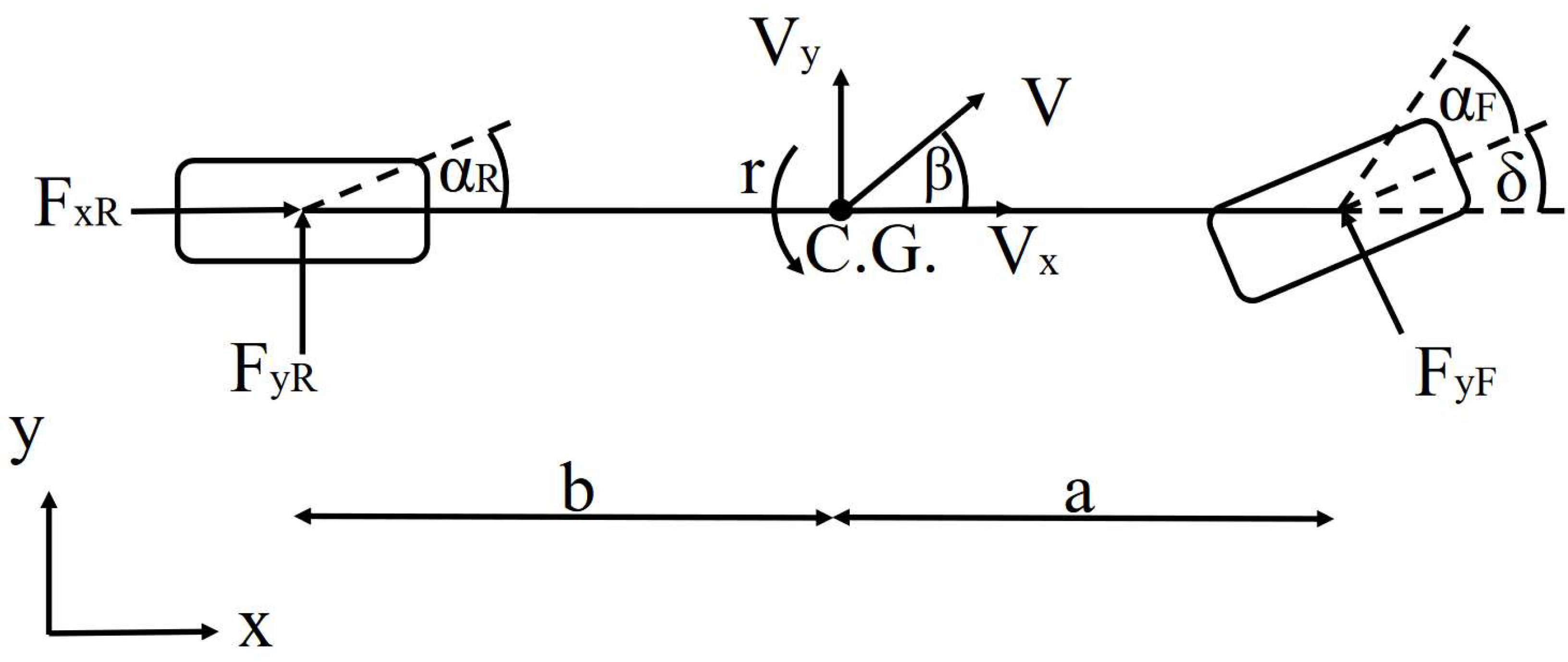
2.1.1. Two-Wheel Planar Vehicle Dynamics

The equations of motion in longitudinal and lateral directions, and the yaw dynamics of the vehicle are presented in differential Equations (1)–(3) based on the Newtonian laws, as described in detail in [21]. Please refer to Appendix A for a better understanding of the applied nomenclature.

$${\stackrel{.}{V}}_x=\frac{1}{m}\left(F_x-F_A\right)+{\mathit{rV}}_y.$$

(1)

$${\stackrel{.}{V}}_y=\frac{1}{m}{F}_y-r{V}_x.$$

(2)

$$\stackrel{.}{r}=\frac{1}{I_z}{M}_z.$$

(3)

The longitudinal (Equation (4)) and lateral (Equation (5)) forces, and the yaw torque (Equation (7)) can be derived from the tire forces as described below, along with the air drag (Equation (6)). The yaw torque (7) is applied at the center of gravity (CoG) of the vehicle.

$$F_x=F_{xF}cos\delta +F_{xR}-F_{yF}sin\delta .$$

(4)

$$F_y=F_{yF}cos\delta +F_{yR}+F_{xF}sin\delta .$$

(5)

$$F_A=\frac{1}{2}A \rho C_A{V}_x^2.$$

(6)

$$M_z=a{F}_{yF}cos\delta -b{F}_{yR}+a{F}_{xF}sin\delta .$$

(7)

The sideslip angle of the front (Equation (8)) and rear (Equation (9)) wheels, and the sideslip angle of the vehicle, which is applied at the center of gravity (Equation (10)), can be calculated in the following way:

$${\alpha }_f=arctan\left(\frac{V_y+ar}{V_x}\right)-\delta ,$$

(8)

$${\alpha }_r=arctan\left(\frac{V_y-br}{V_x}\right),$$

(9)

$$\beta =arctan\left(\frac{V_y}{V_x}\right).$$

(10)

The air drag force F_A is considered zero in the above equations since the speed of drift results in neglectable air drag. Due to small values, rolling and pitching dynamics are also neglected. Since the test vehicle is rear-wheel-driven, and there is no braking during this specific drift maneuver, F_xF is considered zero throughout this paper.

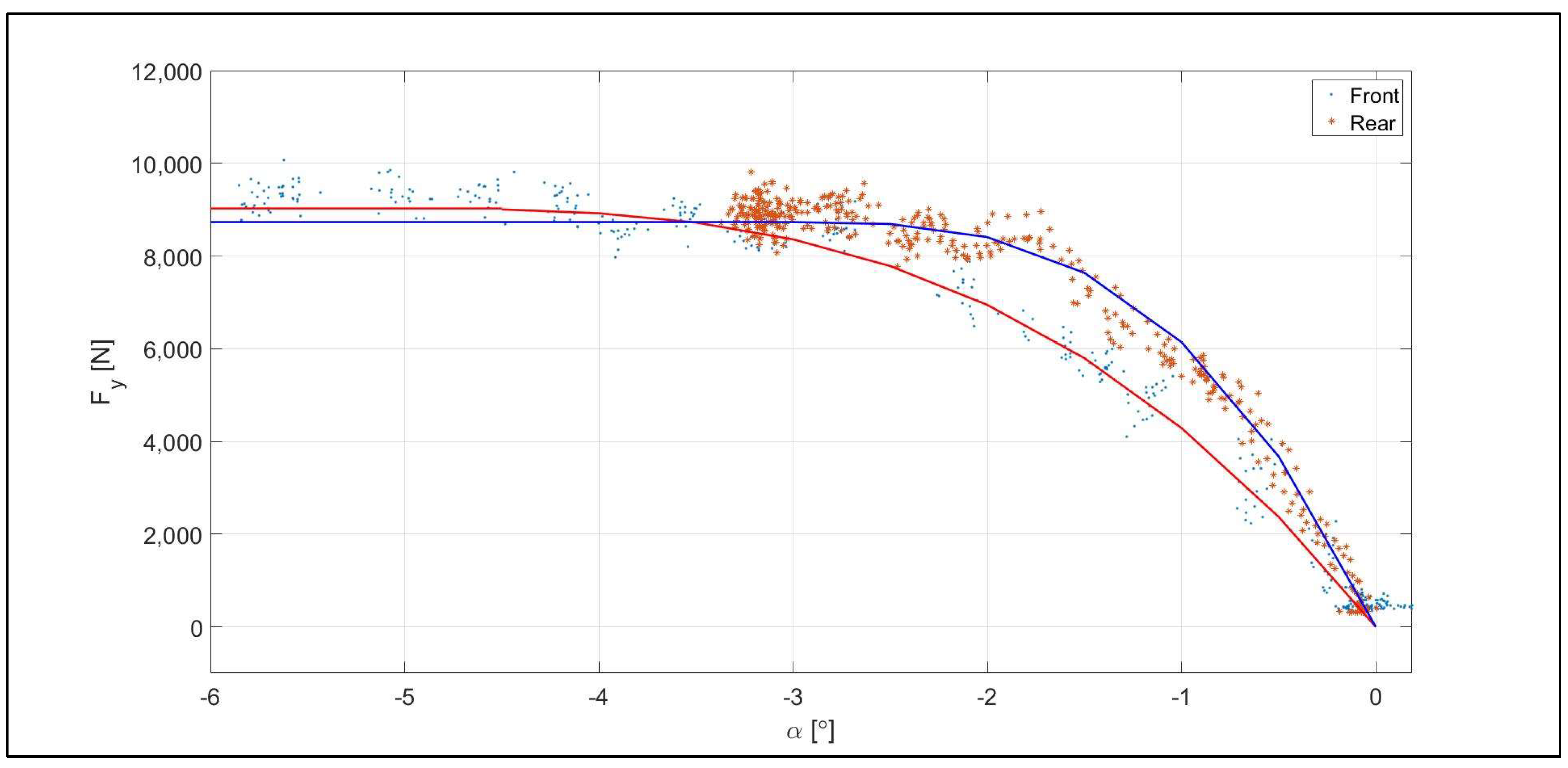
2.1.2. Nonlinear Tire Model

The forces in the above-defined equations awaken in the contact patches of the tires. Owing to the complex, heterogeneous structure of pneumatic rubber tires [22], tire models vary in a wide-scaled spectrum regarding their specific application. According to complexity levels, finite element models [23] and empirical models [24] are also widespread in the literature. For achieving a simple, but meaningful tire model for a control-oriented approach, the so-called brush tire model was selected for calculating the lateral tire force.

The equations below can be used for describing the lateral force of the tires in both saturated and unsaturated phases. Saturation refers to the operating range of the tire, where the change in the lateral slip does not affect the generated force. Physically meaningful consideration was derived in [25,26].

For the front tire where no longitudinal forces are considered, the lateral tire force can be calculated on the basis of the following equations, where ${\alpha }_{sl}$ denotes tire sideslip limit where the tires become saturated:

$$F_{yF}=\{\begin{array}{l}-C_{\alpha F}tan\left(\alpha \right)+\frac{C_{\alpha F}{}^2}{3\mu F_{zF}}tan\left(\alpha \right)\left|tan\left(\alpha \right)\right|-\frac{C_{\alpha F}{}^3}{27{\mu }^2{F}_{zF}^2}tan{\left(\alpha \right)}^3,\left|\alpha \right|\le {\alpha }_{sl}\\ -\mu F_{zF}sgn\left(\alpha \right),\left|\alpha \right|>{\alpha }_{sl}\end{array},$$

(11)

$${\alpha }_{sl\_F}=arctan\left(\frac{3\mu F_{zF}}{C_{\alpha F}}\right).$$

(12)

In the case of the rear tire, a solution must be found to also add the longitudinal forces to the model. A similar approach could be applied that was also used for deriving the lateral forces, although the wheel speeds would appear as additional states in the model. To overcome this matter, the connection between the longitudinal and lateral forces was determined with the friction circle and described by a coupling factor, as suggested in [10]. As stated below, ξ determines the amount of lateral force that can be reached directly from the friction.

$$F_y^{max}=\xi \mu F_{zR}.$$

(13)

$$\xi =\frac{\sqrt{{\left(\mu F_{zR}\right)}^2-F_{xR}{}^2}}{\mu F_{zR}}.$$

(14)

Accordingly, Equation (11) can be augmented to compute both the lateral and the longitudinal forces for the rear tire.

$$F_{yR}=\{\begin{array}{l}-C_{\alpha R}tan\left(\alpha \right)+\frac{C_{\alpha R}{}^2}{3\xi \mu F_{zR}}tan\left(\alpha \right)\left|tan\left(\alpha \right)\right|-\frac{C_{\alpha R}{}^3}{27{\xi }^2{\mu }^2{F}_{zR}^2}tan{\left(\alpha \right)}^3,\left|\alpha \right|\le {\alpha }_{sl}\\ -\xi \mu F_{zR}sgn\left(\alpha \right),\left|\alpha \right|>{\alpha }_{sl}\end{array}.$$

(15)

$${\alpha }_{sl\_R}=arctan\left(\frac{3\xi \mu F_{zR}}{C_{\alpha R}}\right).$$

(16)

2.2. Model Parameter Identification Measurements

Model parameter identification was conducted by the authors. The test vehicle, which was used as a source of model parameter identification measurements, possesses a 3.0 L twin-turbocharged straight-six engine. As for the characteristics of the engine, it is able to produce 550 N·m torque between 2350 and 5230 RPM and 411 HP (302 kW) between 5230 and 7000 RPM. The test vehicle has a rear-wheel drive and a seven-speed dual-clutch automatic transmission.

The position of the center of gravity, depicted in Figure 1, was determined by measuring the axle weights. As a result, 925 kg was measured on the first axle, and 895 kg was measured on the second axle. Taking the total length of the wheelbase, which is 2.69, the position of the center of gravity is situated 1.37 m far away in front of the second axle.

Parameters of the above-defined brush tire model, such as friction coefficients or cornering stiffness, were necessary to identify in advance. For this purpose, the ISO 13674-2 standard was used with ramp steering maneuvers. The measurement was performed from an initial straight line until the vehicle reached a constant velocity of 100 km/h. In the next step, the neutral gear was selected, and a slow, constant velocity ramp was given as an input to the steering wheel. The ZalaZone Dynamical Platform [27] served as a testing ground for the parameter identification. The friction coefficient of its special, dry asphalt was close to 1 in the case of both tires. As a result of the measurements, the cornering stiffness turned out to be 300,000 N/rad for the front tires and 500,000 N/rad for the rear tires [28]. The measured data points and the characteristics of the tires can be seen in Figure 2.

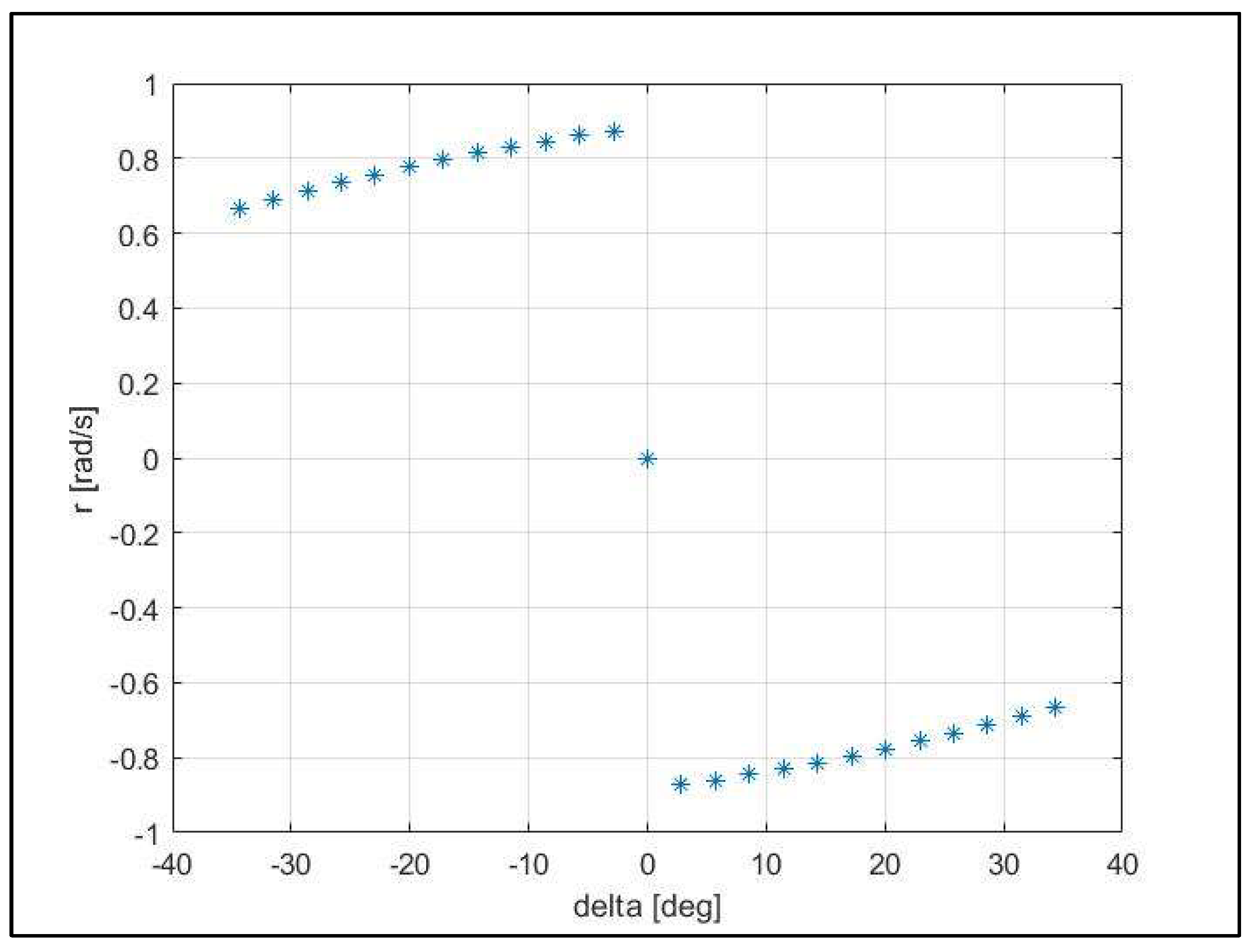
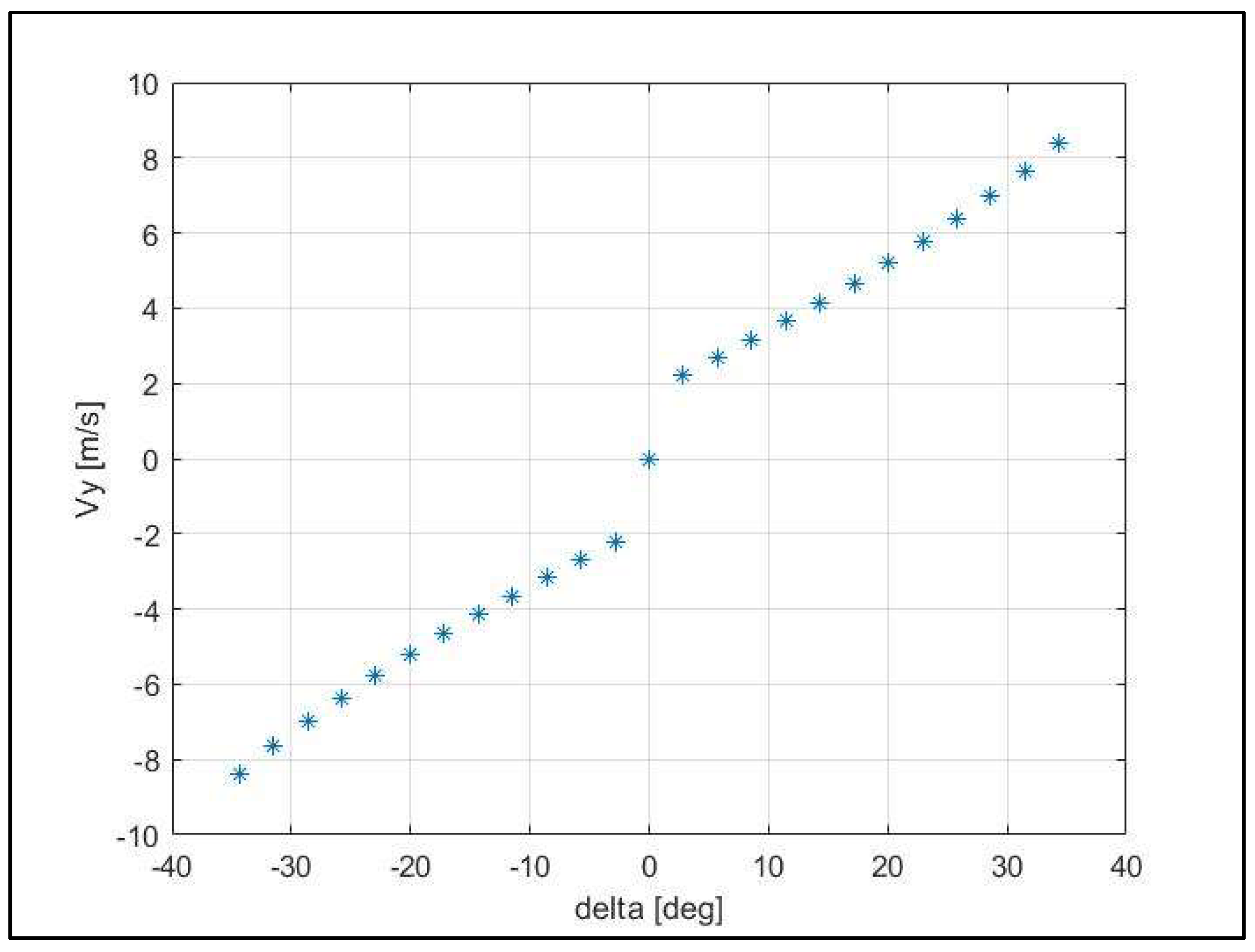
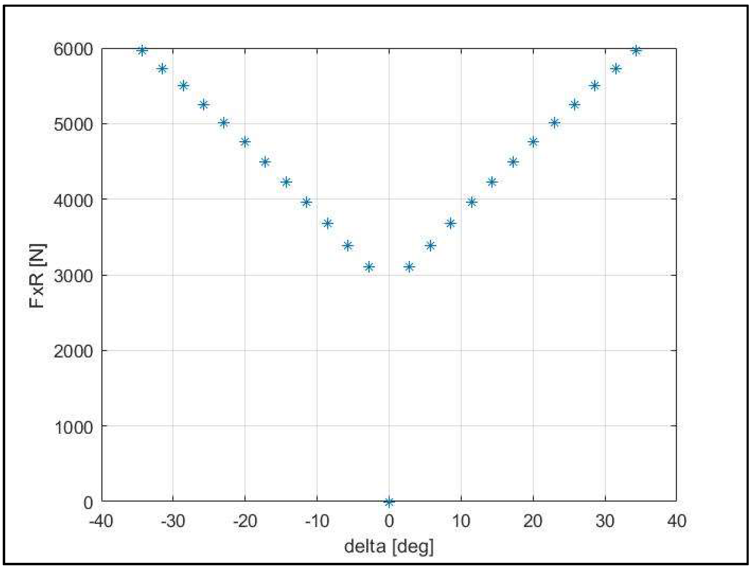
3. Equilibrium Analysis

In this study, steady-state drifting cornering is targeted. It occurs in special locations of the state space, where all the state derivatives are equal to zero, called equilibrium points. With this idea in mind, the equilibria of the system must be determined and analyzed for the desired operation.

According to the three-state bicycle model, the state matrix of the system (Equations (1)–(3)) can be written in the form of

$$x=\left[\begin{array}{c}{V}_y\\ r\\ V_x\end{array}\right],$$

(17)

where the states were chosen as the lateral vehicle speed, yaw rate, and longitudinal vehicle speed.

The control inputs were defined as the roadwheel angle and the rear traction force.

$$u=\left[\begin{array}{c}\delta \\ F_{\mathit{xR}}\end{array}\right].$$

(18)

To locate the equilibria of the system, the following algebraic equation system must be satisfied:

$$\dot{x}=F\left(x^{\mathrm{eq}},u^{\mathrm{eq}}\right)=0.$$

(19)

It can be deduced that our system is an underactuated system since we have one more state than control input. This yields that not all the state derivatives can be driven to zero from an arbitrary point of the state space. Furthermore, considering all the equations, one can see that we have fewer equations than variables; therefore, we need to choose some variables to be fixed in advance. This observation indicates that only specific locations of the state space are solutions of the equation system. To solve this problem, the velocity is set to 10 $\frac{m}{s}$ as a known variable, and the steering angle ranged between −35° and +35° rad with a step size of 2.86°. Figure 3, Figure 4 and Figure 5 show the calculated results of Equation (19) with the described parameters.

For controller performance evaluation, three equilibrium points were chosen to be used in the subsequent sections. Parameter values for the test cases are summarized in

Table 1. Equilibrium points used in the controller evaluation simulations.

Case No.	δ (°)	FxR (N)	Vy (m/s)	r (rad/s)	Vx (m/s)
1	−20.05	4753	−5.21	0.776	10
2	−28.65	5500	−6.99	0.713	10
3	−22.92	5254	−6.36	0.735	10

.

4. Controller Design

In this section, the formulation of the control problem is stated. As previously discussed in Section 1, a MIMO controller is necessary to achieve the desired performance. In this manuscript, an adaptive MPC was designed for this purpose. The state matrices are updated for solving the quadratic problem (QP) at every time step. Updating the state matrices can provide a better control performance during varying environmental conditions due to the utilization of actual model parameter estimates such as the road grip. Moreover, it allows using our controller in multiple equilibria with only one controller.

Below, a system with N_x states and N_u inputs is considered. The system can be described by ordinary differential equations as presented in Section 2.1 and written in the form of Equation (20).

$$\dot{x}=F\left(x,u\right), y=z\left(x,u\right).$$

(20)

4.1. MPC Formulation

Model predictive control is an optimizing control theory that uses the discrete model of the system to predict its behavior in the future. MPC calculates a series of inputs to minimize the predefined cost function at every time step (T_s). When the cost function is minimized, the first element of the calculated control inputs is applied. Crucial parameters are the prediction horizon N_p and the control horizon N_c. N_p defines the capability of the system in terms of how far it can see into the future. The time horizon N_p,_t, which corresponds to the prediction horizon N_p can be written in the following form:

$$N_{p,t}=N_p{T}_s,$$

(21)

where m is a positive integer, and $T_s$ = 10 ms throughout this paper. N_c defines the number of control inputs that can be optimized in one time step. One should carefully set these parameters to see the transient of the system in advance, thereby avoiding unnecessarily high computational needs. The MPC uses full state feedback that minimizes the cost function below.

$$J\left(k\right)=\frac{1}{2}\left({\widehat{x}}^T \stackrel{=}{Q_x}\widehat{x}+{\overline{u}}^T\stackrel{=}{R}\overline{u}+{\widehat{z}}^{T }\stackrel{=}{Q_z}\widehat{z}\right),$$

(22)

where $\widehat{x}$ is the stacked vector of the predicted states, $\widehat{z}$ denotes the performance, and $\overline{u}$ is the control inputs at every time step k. $Q_x=Q_x{}^T \ge 0 \in R^{3\times 3}$, $Q_x=Q_x{}^T \ge 0 \in R^{3\times 3},$ and $R=R^T>0\in R^1$ are weight matrices. Based on this, $\stackrel{=}{Q_x}=diag\left(Q_x,Q_x,\dots Q_x\right)\in R^{N_x{N}_p\times N_x{N}_p}$, $\stackrel{=}{Q_x}=diag\left(Q_z,Q_z,\dots Q_z\right)\in R^{N_x{N}_p\times N_x{N}_p}$, and $\stackrel{=}{R}=diag\left(R,R,\dots R\right)\in R^{N_u{N}_p\times N_u{N}_p}$.

A further advantage of MPC, for instance, over LQ control, is that it handles the constraints of the system directly. Constraints were set in case of the control inputs.

$$-u_{min}<u<u_{max}.$$

(23)

During the simulation, the physical constraints of the test vehicle were taken into consideration. This means that the steering angle δ could range between −35° and +35°, and the driving force F_xR at the rear wheel was between 0 N and 7000 N.

The evolution matrices in Equation (24) can be determined according to [29]. The D selection matrix was zero throughout in this paper. The system state $x\left(k\right)$ is measured at the time step k.

$$\stackrel{\widehat{x}}{\overbrace{\left[\begin{array}{c}x\left(k+1\right)\\ x\left(k+2\right)\\ ⋮\\ x\left(k+Np\right)\end{array}\right]}}=\stackrel{\stackrel{=}{A}}{\overbrace{\left[\begin{array}{c}A\\ A^2\\ ⋮\\ A^{N_p}\end{array}\right]}}x\left(k\right)+\stackrel{\stackrel{=}{B}}{\overbrace{\left[\begin{array}{cccc}B& 0& \cdots & 0\\ AB& B& \cdots & 0\\ ⋮& \cdots & \ddots & ⋮\\ A^{N_p-1}B& \cdots & \dots & B\end{array}\right]}}\stackrel{\overline{u}}{\overbrace{\left[\begin{array}{c}u\left(k\right)\\ u\left(k+1\right)\\ ⋮\\ u\left(k+N_p-1\right)\end{array}\right]}}$$

(24)

The cost function must penalize both the magnitude of the applied control inputs, steering angle, traction force, and deviation of the states from the reference trajectory in order to formulate the optimization problem, the solution of which is the optimal control inputs. The error vector z is the following:

$$\stackrel{\widehat{z}}{\overbrace{\left[\begin{array}{c}z\left(k+1\right)\\ z\left(k+2\right)\\ ⋮\\ z\left(k+Np\right)\end{array}\right]}}=\stackrel{\stackrel{=}{C}}{\overbrace{\left[\begin{array}{cccc}C& 0& \cdots & 0\\ 0& C& \cdots & 0\\ ⋮& \cdots & \mathrm{C}& ⋮\\ 0& \cdots & \dots & C\end{array}\right]}}\stackrel{\widehat{x}}{\overbrace{\left[\begin{array}{c}x\left(k+1\right)\\ x\left(k+2\right)\\ ⋮\\ x\left(k+Np\right)\end{array}\right]}}.$$

(25)

The cost function is calculated by substituting Equations (24) and (25) into Equation (22).

$$J=\frac{1}{2}{\overline{u}}^{T}H\overline{u}+f^T\overline{u}.$$

(26)

For a more detailed derivation, see [28]. The QP problem is formed in the following equation:

$$\underset{u}{\min }\left[\frac{1}{2}{\overline{u}}^{T}H\overline{u}+f^T\overline{u}\right],$$

(27)

subject to

$$-0.6<u_1<0.6,$$

(28)

$$0<u_2<7000.$$

(29)

4.2. Successive Linearization

Traditional MPC works on linear and discrete models. Nonetheless, the vast majority of dynamical systems are nonlinear, which is the case of the presented vehicle model introduced in Section 2.1. To be able to create an MPC control scheme, it is reasonable to linearize the nonlinear system and discretize the continuous system afterward. Successive linearization was selected according to [30]. Successive linearization is a key tool to make our model adaptive to environmental and conditional changes in real time. Successive linearization is a linearization method followed by discretization. The idea is to create a linear MPC for every time step and make it adaptive to the changing conditions by updating the model that the MPC uses to formulate the QP problem, instead of using a more complex control scheme like nonlinear MPC in [31].

The system described in Equation (20) can be linearized in specific operating points by knowing its gradient. One can interpret it as Jacobian linearization. According to the aforementioned specifications, the state matrices of the linearized system can be derived as follows:

$$A_c\left(i,j\right)=\frac{\partial F_i}{\partial x_j},B_c\left(i,j\right)=\frac{\partial F_i}{\partial u_j},$$

(30)

$$C_c\left(i,j\right)=\frac{\partial z_i}{\partial x_j},D_c\left(i,j\right)=\frac{\partial z_i}{\partial u_j}.$$

(31)

By knowing the operating points at every time step, the matrices in Equations (30) and (31) can be determined in numerical form. Since MPC works on discrete systems, discretization is required.

The linear continuous system of Equations (30) and (31) can be discretized as defined in Equations (32)–(34).

$$A_d=e^{A_c{T}_s}.$$

(32)

$$B_d=A_c^{-1}\left(e^{A_c{T}_s}-I\right)B_c.$$

(33)

$$C_d=C_c,D_d=D_c.$$

(34)

Equations (32)–(34) can be substituted into Equations (24) and (25) at every time step.

A MATLAB and Simulink environment was used for model and controller implementation (the implemented MPC controller and the nonlinear vehicle model are marked in blue in Figure 6), as well as for software-in-loop testing. In order to appropriately tune the weight matrices of Equation (22), a simple linear MPC was created for one equilibrium. Since the aim is to control a nonlinear system with a linear controller around an equilibrium, one should take coordinate system transformation into consideration as a result of Jacobian linearization. Coordinate system transformation was applied according to [32]. The control scheme is depicted in Figure 6. Blocks responsible for coordinate transformation between the controller and the vehicle model are marked in yellow.

5. Simulation Results

In this section, the simulation results are revealed. The first test case was created to tune the parameters of the controller and test its performance. In the second test case, the vehicle was driven through multiple equilibria. Lastly, the alteration of the road surface was considered while driving through multiple equilibria.

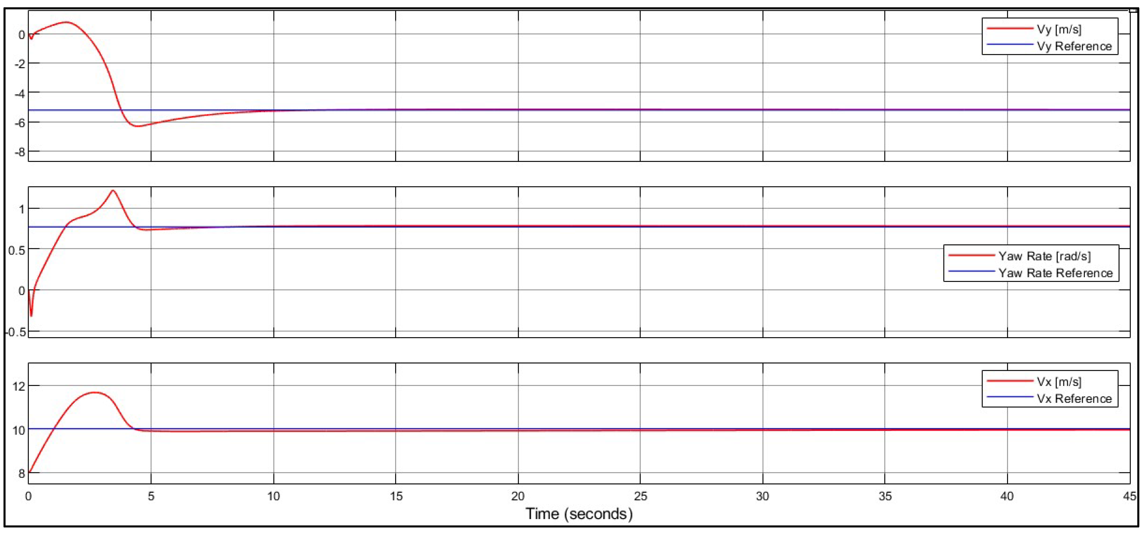
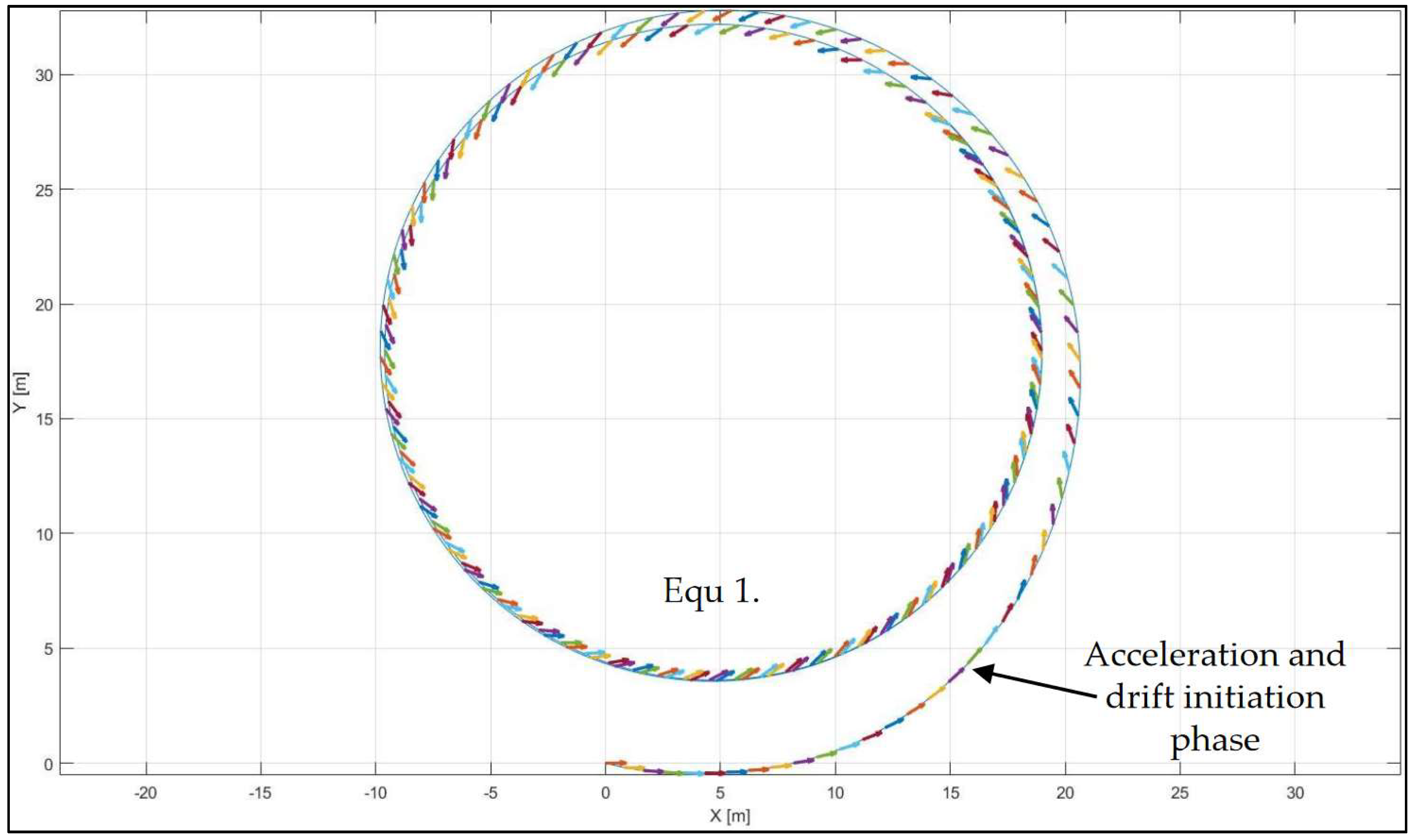
5.1. Steady-State Drift in a Single Equilibrium

Firstly, the control scheme was tested only using Case No. 1 of Table 1 (Equation (1)). This was an important step in order to tune the weight matrices. A PI (proportional–integral) cruise controller was used to accelerate the vehicle from 0 to 8 m/s, after which the control was given to the MPC drift controller. The controller was able to drive the car into a drift state and keep it there simultaneously. Figure 7 shows the simulation results after 8 m/s was reached. The controller needed to cope with the task of accelerating the vehicle by 2 m/s to reach the desired drifting speed. It can be deduced from the results that the designed linear controller was capable of controlling the defined nonlinear system around the desired equilibrium after the proper tuning. This was proven by the simulations where the vehicle performed a high-sideslip cornering motion, as depicted in Figure 8. The movement of the vehicle can also be tracked in this figure. Firstly, the drift controller took over the control at (0,0), after which there was an acceleration period. When all the states were driven to the operating points, the steady-state drift was maintained.

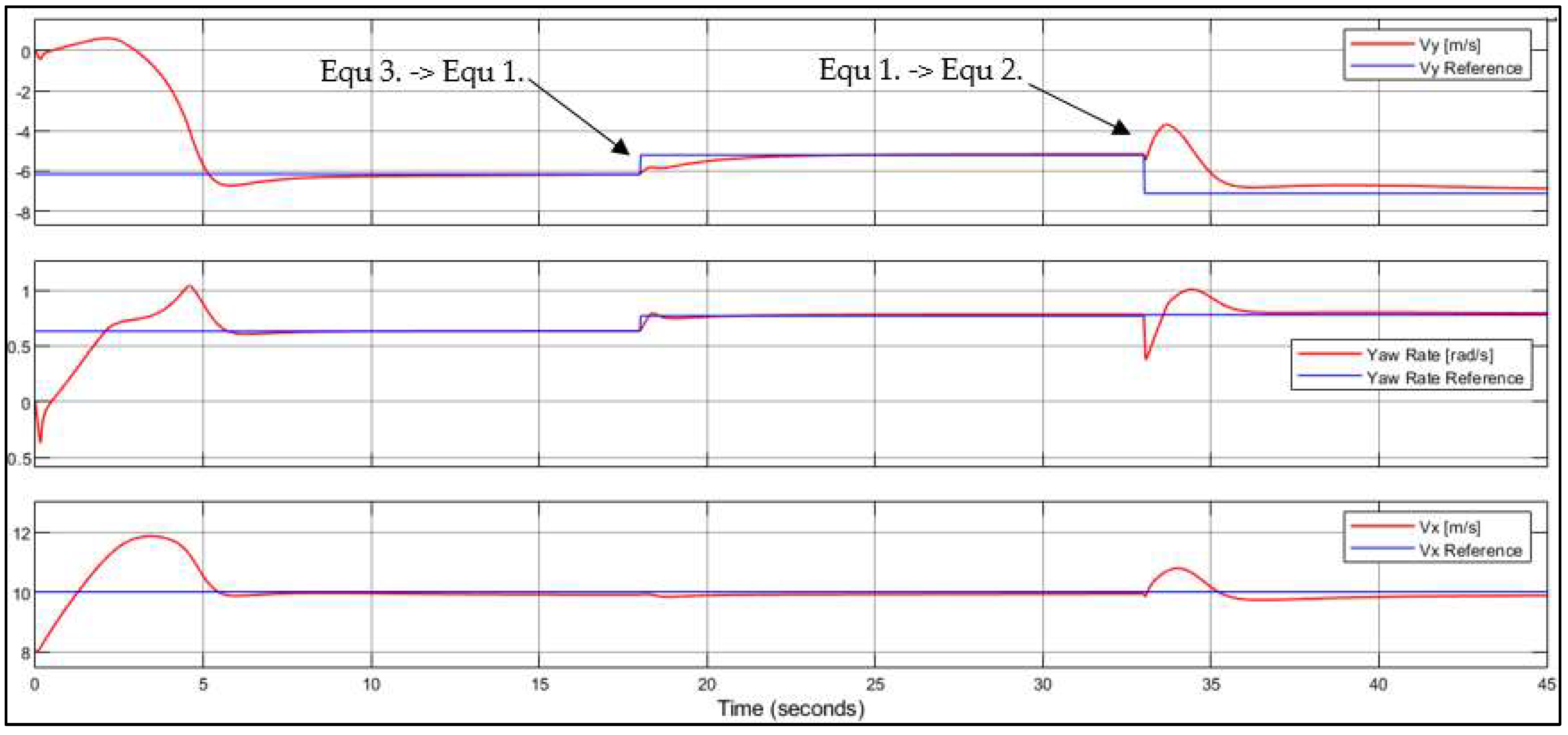
5.2. Steady-State Drift in Multiple Equilibria

The controller introduced in Section 5.1 was able to maintain the system at the desired operating point. However, it performed poorly in other segments of the state space. The adaptive MPC structure can be a solution for this limitation. This section points out the advantages of adaptive MPC over linear MPC for multi-operating point purposes.

The second step after Section 5.1 was to drift around three different equilibria. In this case, the system was updated, and a new MPC was formed online at every time step. The MPC could not only keep the vehicle at the limit of handling, but it was also able to drive the system from one equilibrium to another. The order of the steady points was based on the idea to test the robustness of the controller. First of all, the controller needed to accelerate the system from 8 m/s to 10 m/s while driving it into a drift state. Furthermore, after drifting in the first circle, the controller needed to drive the vehicle into a circle with a smaller radius and into a considerably bigger one after that. The transition in the first case from Equation (3) to Equation (1) was relatively smaller (these were closer operating points) than that from Equation (1) to Equation (2), as can be seen in Figure 9 by examining the overshoots. The controller was able to cope with both acceleration and deceleration tasks. Figure 10 depicts the control inputs during steady-state drift at the operating points. As can be seen, the control inputs were the same in the steady-state cases as the precalculated values in Table 1.

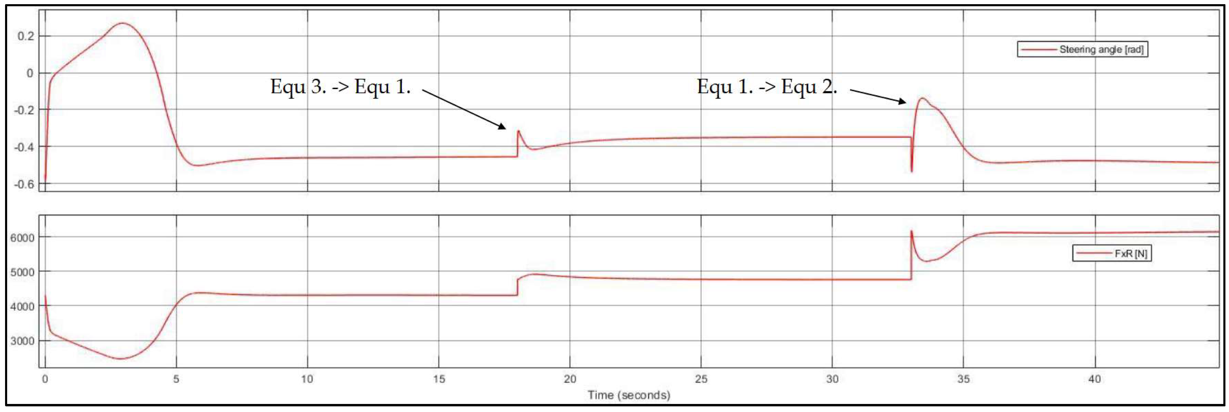
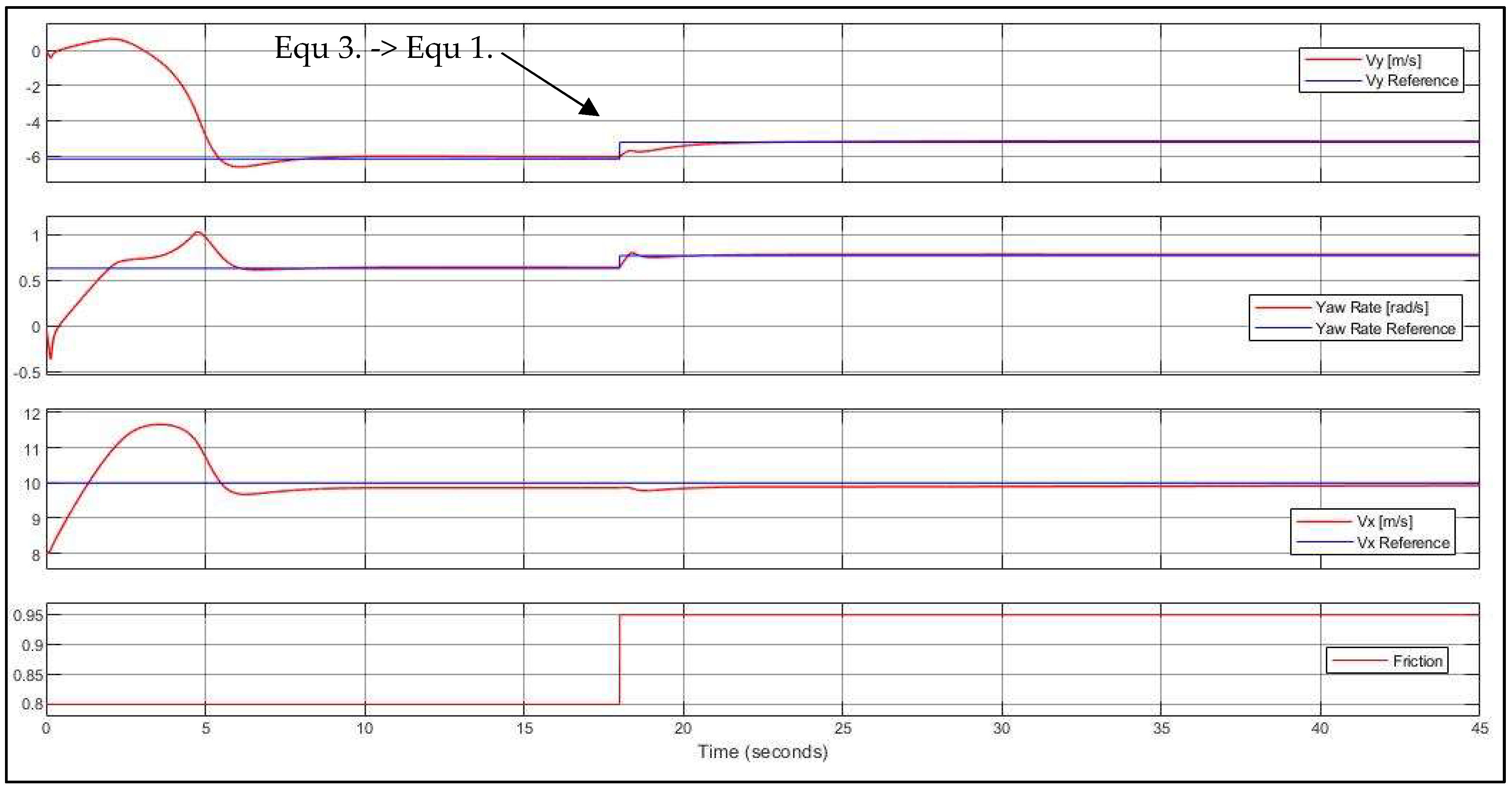
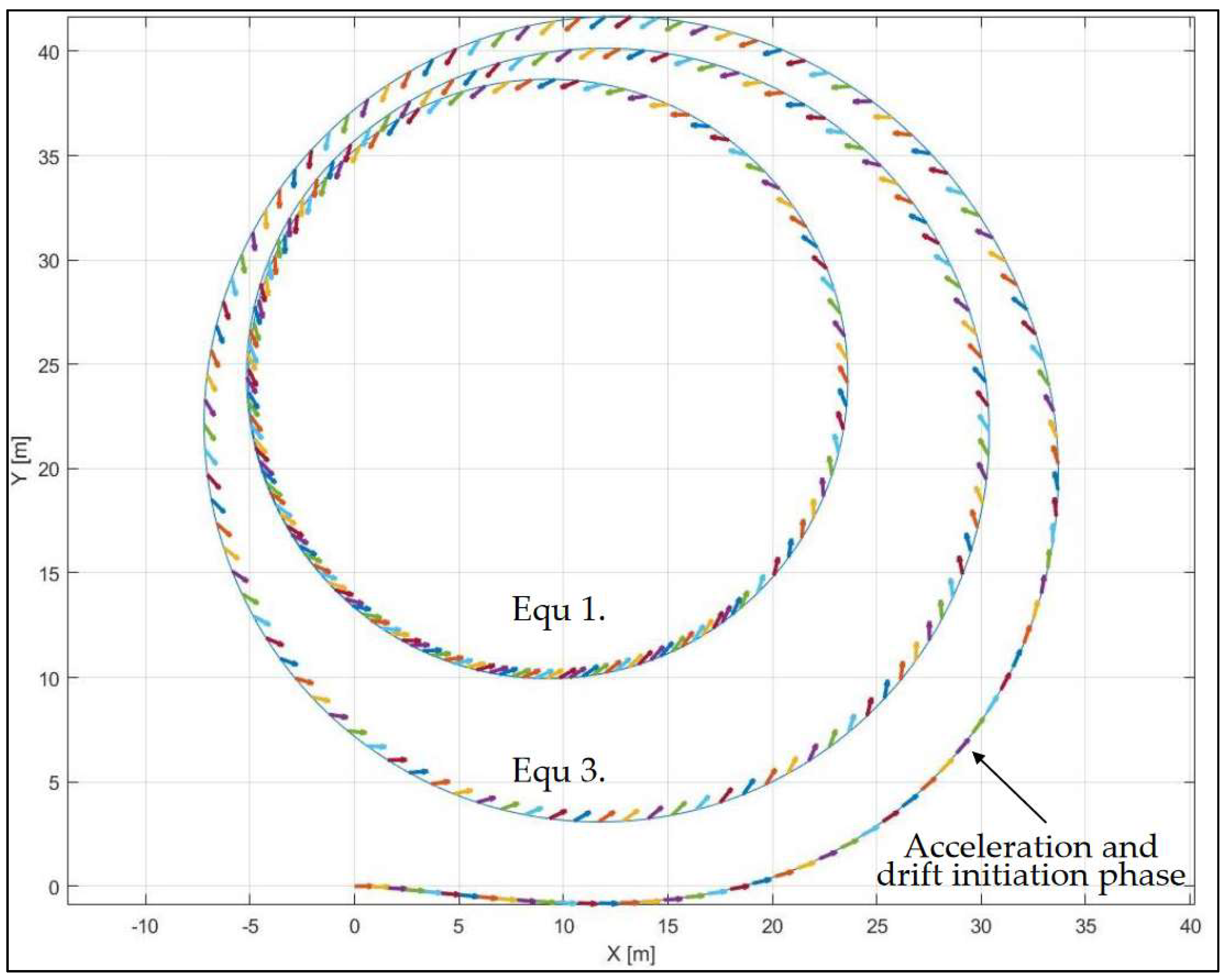
5.3. Drifting on Varying Road Surfaces

In real-life scenarios, changing road surfaces is a common occurrence. Moreover, during drifting, the vehicle can also go off-road or across wet asphalt areas. The varying friction of road surfaces raises many challenges for autonomous vehicles. Road surface estimation is an active topic in the field of autonomous vehicle development. Machine learning is a promising methodology for road surface estimation, as shown in [33,34,35]. A new idea was proposed in [35] based on a machine-learning approach to estimate road surface. The authors introduced a methodology that relies on large datasets that can be collected using onboard sensors or dynamic simulations. Online road surface estimation is an essential extension of the proposed method introduced in Section 5.2. Nevertheless, it is beyond the scope of the present work. Hence, preset friction coefficients were used for testing the adaptability of the software.

Simulations confirmed the fact that the tolerance of the linear controller was limited toward road changes. Setting the friction coefficient of the road surface to 0.8 from 0.95, for instance, resulted in poor performance or even instability. Adaptive topology can also be used to eliminate this problem. By having an estimation of the road surface, the friction coefficient can be updated along with the other parameters to provide a more accurate model for the MPC to work on. Road friction is considered a variable in the state matrices updated at every time step before passing them to the MPC for prediction.

The friction coefficient was changed as a step, assuming a sudden alteration of the road surface. The change was made at the same time when the controller attempted to drive the system into a new equilibrium. The grip suddenly changed from 0.8 to 0.95, which is roughly equivalent to a wet to dry road transition. Overall, the alteration of the road friction could be interpreted as a special type of transition between equilibria. Figure 11 shows the evolution of the states during the test case, while Figure 12 depicts the trajectory traveled. Despite the sudden change in the operating conditions, the proposed adaptive MPC controller was able to precisely stabilize both targeted drift equilibria by utilizing the available information of the road grip.

6. Conclusions

In this article, the authors highlighted the importance of vehicle motion control at handling limits and automated drifting as one of the critical developments of fully autonomous vehicles of the future, aiming at improved road safety. Vehicle automated drifting capabilities were demonstrated during different operating conditions with a systematic controller development process, as outlined below. The handling of changing road conditions and vehicle model nonlinearities is among the key advantages of the proposed adaptive MPC control framework. In Section 2, a nonlinear dynamic vehicle model and a nonlinear tire model were introduced for control-oriented purposes, and the parameter identification was carried out. In Section 3 and Section 4, the control scheme and the updating strategy were explained in detail.

In Section 5.1, the weight matrices were determined using a single equilibrium for testing. It was shown that a linear MPC is capable of driving the nonlinear system into the desired drifting equilibrium, keeping it there with the appropriate tuning.

Linear MPC is a simpler control methodology compared to nonlinear MPC, but it performs poorly if the change in vehicle dynamic behavior is far from the design point due to nonlinearities or when it faces parameter variations (road surface changes). According to the proposed idea, these drawbacks can be eliminated by updating the discrete model of the vehicle, reformulating the MPC in an adaptive way, and utilizing measured or estimated model parameter values. This allows using the same MPC structure by updating it instead of using a more different linear MPC and a decision controller for drifting in multiple equilibria as a gain scheduling.

Another advantage of this method in vehicle motion control is directly handling changes in the road surface. A slight or abrupt variation in friction is a common occurrence in real-life driving scenarios. This paper showed that the controller could handle not only various transitions between multiple equilibria but also a simultaneous change in the road grip.

A reasonable next step of the work is to extend the proposed framework with trajectory-planning and -tracking capabilities and possibly online road surface estimation to demonstrate advantages in critical road safety scenarios.

References

1. Ágoston, G.; Madleňák, R. Road Safety Macro Assessment Model: Case Study for Hungary. Period. Polytech. Transp. Eng. 2021, 49, 89–92. [Google Scholar] [CrossRef] [Green Version]
2. Ghadi, M.Q.; Török, Á. Evaluation of the Impact of Spatial and Environmental Accident Factors on Severity Patterns of Road Segments. Period. Polytech. Transp. Eng. 2020, 49, 146–155. [Google Scholar] [CrossRef] [Green Version]
3. Hegedűs, T.; Németh, B.; Gáspár, P. Challenges and Possibilities of Overtaking Strategies for Autonomous Vehicles. Period. Polytech. Transp. Eng. 2020, 48, 320–326. [Google Scholar] [CrossRef]
4. Paden, B.; Cap, M.; Yong, S.Z.; Yershov, D.; Frazzoli, E. A Survey of Motion Planning and Control Techniques for Self-Driving Urban Vehicles. IEEE Trans. Intell. Veh. 2016, 1, 33–55. [Google Scholar] [CrossRef] [Green Version]
5. Wu, N.; Huang, W.; Song, Z.; Wu, X.; Zhang, Q.; Yao, S. Adaptive dynamic preview control for autonomous vehicle trajectory following with ddp based path planner. In Proceedings of the 2015 IEEE Intelligent Vehicles Symposium (IV), Seoul, Korea, 28 June–1 July 2015; pp. 1012–1017. [Google Scholar]
6. Bacha, S.; Saadi, R.; Ayad, M.Y.; Aboubou, A.; Bahri, M. A review on vehicle modeling and control technics used for autonomous vehicle path following. In Proceedings of the 2017 International Conference on Green Energy Conversion Systems (GECS), Hammamet, Tunisia, 23–25 March 2017; pp. 1–6. [Google Scholar]
7. Zhang, B.; Chen, G.; Zong, C. Path tracking of full drive-by-wire electric vehicle based on model prediction control. In Proceedings of the 2018 IEEE Intelligent Vehicles Symposium (IV), Changshu, China, 26–30 June 2018; pp. 868–873. [Google Scholar]
8. Velenis, E.; Frazzoli, E.; Tsiotras, P. On steady-state cornering equilibria for wheeled vehicles with drift. In Proceedings of the 48h IEEE Conference on Decision and Control (CDC) Held Jointly with 2009 28th Chinese Control Conference, Shanghai, China, 15–18 December 2009; pp. 3545–3550. [Google Scholar]
9. Velenis, E.; Frazzoli, E.; Tsiotras, P. Steady-state cornering equilibria and stabilisation for a vehicle during extreme operating conditions. Int. J. Veh. Auton. Syst. 2010, 8, 10. [Google Scholar] [CrossRef]
10. Hindiyeh, R.Y. Dynamics and Control of Drifting in Automobiles. Ph.D. Thesis, Stanford University, Stanford, CA, USA, 2013. [Google Scholar]
11. Bardos, A.; Domina, A.; Szalay, Z.; Tihanyi, V.; Palkovics, L. MIMO controller design for stabilizing vehicle drifting. In Proceedings of the IEEE Joint 19th International Symposium on Computational Intelligence and Informatics and 7th IEEE International Conference on Recent Achievements in Mechatronics, Automation, Computer Sciences and Robotics, Szeged, Hungary, 14–16 November 2019. [Google Scholar]
12. Wachter, E.; Alirezaei, M.; Bruzelius, F.; Schmeitz, A. Path control in limit handling and drifting conditions using State Dependent Riccati Equation technique. Proc. Inst. Mech. Eng. Part D J. Automob. Eng. 2019, 234, 783–791. [Google Scholar] [CrossRef]
13. Xu, D.; Wang, G.; Qu, L.; Ge, C. Robust Control with Uncertain Disturbances for Vehicle Drift Motions. Appl. Sci. 2021, 11, 4917. [Google Scholar] [CrossRef]
14. Guo, K.; Lu, D. UniTire: Unified tire model for vehicle dynamic simulation. Veh. Syst. Dyn. 2007, 45, 79–99. [Google Scholar] [CrossRef]
15. Bai, G.; Meng, Y.; Liu, L.; Luo, W.; Gu, Q.; Li, K. A New Path Tracking Method Based on Multilayer Model Predictive Control. Appl. Sci. 2019, 9, 2649. [Google Scholar] [CrossRef] [Green Version]
16. Chen, C.; Guo, J.; Guo, C.; Chen, C.; Zhang, Y.; Wang, J. Adaptive Cruise Control for Cut-In Scenarios Based on Model Predictive Control Algorithm. Appl. Sci. 2021, 11, 5293. [Google Scholar] [CrossRef]
17. Zhang, X.; Göhlich, D. Integrated Traction Control Strategy for Distributed Drive Electric Vehicles with Improvement of Economy and Longitudinal Driving Stability. Energies 2017, 10, 126. [Google Scholar] [CrossRef] [Green Version]
18. Zhai, L.; Hou, R.; Sun, T.; Kavuma, S. Continuous Steering Stability Control Based on an Energy-Saving Torque Distribution Algorithm for a Four in-Wheel-Motor Independent-Drive Electric Vehicle. Energies 2018, 11, 350. [Google Scholar] [CrossRef] [Green Version]
19. Park, J.; Jang, I.G.; Hwang, S.-H. Torque Distribution Algorithm for an Independently Driven Electric Vehicle Using a Fuzzy Control Method: Driving Stability and Efficiency. Energies 2018, 11, 3479. [Google Scholar] [CrossRef] [Green Version]
20. Joa, E.; Cha, H.; Hyun, Y.; Koh, Y.; Yi, K.; Park, J. A new control approach for automated drifting in consideration of the driving characteristics of an expert human driver. Control. Eng. Pr. 2020, 96, 104293. [Google Scholar] [CrossRef]
21. Reza, N.J. Advanced Vehicle Dynamics; Springer: Cham, Switzerland, 2019; pp. 143–144. ISBN 978-3-030-13060-2. [Google Scholar]
22. Lugaro, C.; Alirezaei, M.; Konstantinou, I.; Behera, A. A Study on the Effect of Tire Temperature and Rolling Speed on the Vehicle Handling Response; SAE Technical Paper 2020-01-1235; SAE International: Warrendale, PA, USA, 14 April 2020. [Google Scholar]
23. Helnwein, P.; Liu, C.; Meschke, G.; Mang, H. A new 3-d finite element model for cord-reinforced rubber composites application to analysis of automobile tires. Finite Elem. Anal. Des. 1993, 14, 1–16. [Google Scholar] [CrossRef]
24. Pacejka, H.B.; Bakker, E. The magic formula tyre model. Veh. Syst. Dyn. 1992, 21 (Suppl. S1), 1–18. [Google Scholar] [CrossRef]
25. Fiala, E. Lateral forces on rolling pneumatic tires. Z. VDI 1954, 96, 973–979. [Google Scholar]
26. Hadekel, R. The mechanical characteristics of pneumatic tyres. In Sand T Memo TPA3/TIB; National Association of Housing & Redeve: Washington, DC, USA, 1952. [Google Scholar]
27. Szalay, Z.; Hamar, Z.; Nyerges, Á. Novel design concept for an automotive proving ground supporting multilevel CAV development. Int. J. Veh. Des. 2019, 80, 1–22. [Google Scholar] [CrossRef]
28. Bardos, A.; Domina, A.; Tihanyi, V.; Szalay, Z.; Palkovics, L. Implementation and experimental evaluation of a MIMO drifting controller on a test vehicle. In Proceedings of the 2020 IEEE Intelligent Vehicles Symposium (IV), Las Vegas, NV, USA, 19 October–13 November 2020; pp. 1472–1478. [Google Scholar]
29. Varga, B.; Tettamanti, T.; Kulcsár, B. Optimally combined headway and timetable reliable public transport system. Transp. Res. Part C Emerg. Technol. 2018, 92, 1–26. [Google Scholar] [CrossRef]
30. Zhakatayev, A.; Rakhim, B.; Adiyatov, O.; Baimyshev, A.; Varol, H.A. Successive linearization based model predictive control of variable stiffness actuated robots. In Proceedings of the 2017 IEEE International Conference on Advanced Intelligent Mechatronics (AIM), Munich, Germany, 3–7 July 2017; pp. 1774–1779. [Google Scholar]
31. Grüne, L.; Pannek, J. Nonlinear Model Predictive Control. In Nonlinear Model Predictive Control: Theory and Algorithms; Springer: Cham, Switzerland, 2017; pp. 45–69. [Google Scholar]
32. Roubal, J.; Husek, P.; Stecha, J. Linearization: Students Forget the Operating Point. IEEE Trans. Educ. 2009, 53, 413–418. [Google Scholar] [CrossRef]
33. Panahandeh, G.; Ek, E.; Mohammadiha, N. Road friction estimation for connected vehicles using supervised machine learning. In Proceedings of the 2017 IEEE Intelligent Vehicles Symposium (IV), Los Angeles, CA, USA, 11–14 June 2017; pp. 1262–1267. [Google Scholar]
34. Roychowdhury, S.; Zhao, M.; Wallin, A.; Ohlsson, N.; Jonasson, M. Machine Learning Models for Road Surface and Friction Estimation using Front-Camera Images. In Proceedings of the 2018 International Joint Conference on Neural Networks (IJCNN), Rio de Janeiro, Brazil, 8–13 July 2018; pp. 1–8. [Google Scholar]
35. Fényes, D.; Németh, B.; Gáspár, P.; Szabó, Z. Road surface estimation based LPV control design for autonomous vehicles. IFAC-PapersOnLine 2019, 52, 120–125. [Google Scholar] [CrossRef]
Figure 1. Bicycle model notations used in the equations.
Energies 14 06667 g001
Figure 2. The measured tire curves for the front and rear tires.
Energies 14 06667 g002
Figure 3. Equilibrium lateral speeds as a function of roadwheel angle.
Energies 14 06667 g003
Figure 4. Equilibrium yaw rates as a function of roadwheel angle.
Energies 14 06667 g004
Figure 5. Equilibrium traction forces versus roadwheel angle.
Energies 14 06667 g005
Figure 6. The control scheme.
Energies 14 06667 g006
Figure 7. Drift scenario around equilibrium Case No. 1.
Energies 14 06667 g007
Figure 8. The heading of the vehicle during steady-state drift in equilibrium Case No. 1.
Energies 14 06667 g008
Figure 9. Evolution of states while settling in the three different equilibria.
Energies 14 06667 g009
Figure 10. Control inputs during the test while reaching the targeted three different equilibria.
Energies 14 06667 g010
Figure 11. Vehicle states during the test case showing the handling of rapid change of road surface grip.
Energies 14 06667 g011
Figure 12. Path and heading of the vehicle in the changing road grip test case.
Energies 14 06667 g012